Abstract
Graph convolutional networks (GCNs) have been successfully applied to learning tasks on graph-structured data. However, most traditional GCNs based on graph convolutions assume homophily in graphs, which leads to a poor performance when dealing with heterophilic graphs. Although many novel methods have recently been proposed to deal with heterophily, the effect of homophily and heterophily on classifying node pairs is not clearly separated in existing approaches and inevitably influences each other. To deal with various types of graphs more accurately, in this work we propose a new GCN-based model that leverages the explicitly estimated homophily and heterophily degree between node pairs and adaptively guides the propagation and aggregation of signed messages. We also design a pre-training process to learn homophily and heterophily degree from both original node attributes that are graph-agnostic and the localized graph structure information by using Deepwalk that reflects graph topology. Extensive experiments on eight real-world benchmarks demonstrate that the new approach achieves state-of-the-art results on three homophilic graph datasets and outperforms baselines on five heterophilic graph datasets.
1. Introduction
Graph convolutional networks (GCNs) [1], and their variants, such as GAT [2], GraphSage [3] and GIN [4], have made great progress in network analysis tasks [5] and have been widely-used in many fields, such as natural language processing [6,7], recommendation systems [8,9], bioinformatics [10] and so on.
The design of traditional GCN-based methods, such as GAT, GraphSAGE and GIN, is based on the homophily assumption, which means that the connected nodes in a graph more likely belong to the same category or have similar features [1,11]. The traditional GCN-based methods reflect the assumption of a message-passing mechanism [5,12], where connected nodes propagate features to each other as messages, and each node aggregates the node features of neighbors and then combines the aggregated message and ego features to update the node representation [1,2,4,5]. For each node, the aggregation and update process can be viewed as a weighted sum of ego features and all neighbor’s features, and the neighbor’s features are always assigned positive coefficients when calculating the weighted sum. From the perspective of spectral approaches [5,13,14], the results in [15,16] show that the typical message-passing mechanism of the GCNs above actually acts as a low-pass filter, which filters out high-pass signals and retains the low-pass signals. It causes the representations of connected nodes to tend to be similar and easier to be classified as the same category. Under this assumption, the traditional GCN-based methods have shown good predictive accuracy of node classification tasks on homophilic graphs.
However, there are many graphs in the real-world where a large number of neighbouring nodes belong to different categories, also known as heterophilic graphs. For example, on e-commerce websites, a fraudster is more inclined to interact with ordinary users than with another fraudster [17]. In dating networks, users tend to establish relationships with the opposite gender. Studies have shown that many traditional GCN models are ineffective on heterophilic graphs, especially for semi-supervised node classification tasks [18,19]. As shown in Figure 1a, consider updating the node feature of that has two neighbours and . By applying the traditional message-passing method, the updated representation of node is obtained by adding the node features of and to its self-representation, respectively. After updating, the node feature of becomes closer to that of both and , which makes it difficult to distinguish between nodes and that belong to different categories.
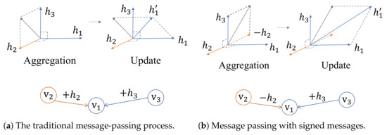
Figure 1.
An illustration of two message-passing processes for updating the node feature of , where are mutually perpendicular three-dimensional feature vectors of nodes , and the node color indicates their category, and is the updated node feature of after aggregating , and combining with .
Recently, many novel GCN-based methods have been proposed to deal with heterophily. Notably, FAGCN [20] takes the perspective of graph signal processing [21] and explores both low-pass filters and high-pass filters in the model design. By connecting to the spatial domain that the process of low-pass filtering represents, the sum of node features with neighbours and the process of high-pass filtering represent the difference of node features between neighbouring nodes; it uses a self-gating mechanism to learn the signed coefficients of the messages. HOG-GCN [22] and BM-GCN [23] explore the estimated homophily degree between node pairs to guide the propagation of positive messages but do not consider how to guide the propagation of negative messages, which is often important in heterophilic graphs. Consider again the example in Figure 1b, if we introduce signed messages during the message-passing process, the updated representation of node is closer to that of its homophilic neighbor and away from that of its heterophilic neighbor as expected. We also observe that the above methods have a common limitation in that the effects of homophily and heterophily on classifying node pairs are not clearly separated in their learning approaches and inevitably influence each other.
In this paper, we aim to design a new model that works well on either homophilic or heterophilic graphs for semi-supervised node classification tasks. Comparing the existing approaches and inspired by the above models, especially FAGCN and HOG-GCN, we would like to leverage explicitly the estimated homophily and heterophily degree between node pairs to adaptively guide the propagation and aggregation of signed messages, respectively. In particular, positive messages are aggregated from homophilic neighbors, and negative messages are aggregated from heterophilic neighbors. To overcome the limitation that the categories of most nodes are unknown in semi-supervised node classification tasks, we pre-train estimators to calculate both the homophily and the heterophily degree of node pairs, which reflect the probability that neighbouring nodes belong to the same category and different categories, respectively. We also propose to learn estimators from both original node attributes that are graph-agnostic and the localized graph structure information by using Deepwalk [24] that reflects graph topology. These two estimators are jointly used in our learning process. We adopt a two-stage training method to train our proposed model, in which the estimators are pre-trained in the first stage, and the GCN module together with the pre-trained estimators are jointly trained in the second stage. That is, the estimators are fine-tuned when training the GCN module.
To summarize, the main contributions of this paper are as follows:
- 1
- We propose an improved GCN-based message-passing mechanism which explores the explicitly estimated homophily and heterophily degree to adaptively guide the passing of positive and negative messages, respectively. The improved mechanism makes the learned representations of nodes which belong to different categories easier to be distinguished in both homophilic and heterophilic graphs.
- 2
- We propose extracting localized structure information in graphs by using Deepwalk which is explored to pre-train an estimator. The estimator as well as the pre-trained estimator learned from original node attributes are jointly used and give us an approach to estimate appropriate homophily and heterophily degree of node pairs.
- 3
- We then design a new Graph Convolutional Network Guided by Explicitly-Estimated Homophily and Heterophily Degree called GCN-EHHD based on the above components. Extensive experiments on eight real-world benchmarks demonstrate the effectiveness of our model. Specifically, GCN-EHHD achieves state-of-the-art results on three homophilic graph datasets and outperforms baselines on five heterophilic graph datasets.
The rest of the paper is organized as follows. In Section 2, we briefly introduce the related work on tackling semi-supervised node classification tasks on heterophilic graphs. In Section 3, we define the semi-supervised node classification tasks and describe the details of our proposed GCN-EHHD. In Section 4, we demonstrate the effectiveness of our proposed approach by comprehensive experiments and an ablation study on real-world datasets. Finally, we conclude with future work in Section 5.
2. Related Work
There are two major GCN-based approaches for tackling learning problems on heterophilic graphs. One is to mine more supplemental nodes when updating a node feature in the message-passing process, which act as those directly-connected neighbors for propagating messages to the node and participate in aggregation and updating of node representation. Geom-GCN [18] maps each node to the latent space and takes the nodes whose distance from the node is less than the setting value in the latent space as the supplemental nodes. NL-GNN [25] utilizes an attention-guided sorting method to choose the supplemental nodes. It defines a learnable calibration vector and adopts an attention mechanism to calculate the attention scores of each node representation and the calibration vector. All nodes are sorted according to their attention scores. For each node, the other nodes whose attention scores are similar are chosen as the supplemental nodes. In addition to the above methods, there are some works that choose the higher-order neighbors in the graph as supplemental nodes. They are based on the observation that for nodes in heterophilic graphs, the first-order neighbors are often heterophilic, but the higher-order neighbors are likely to be homophilic [26]. MixHop [19] chooses two-hop neighbors as the supplemental nodes for message passing. In the layers of MixHop, the messages from different hops neighbors are linearly transformed by different weights and then concatenated. H2GCN [26] chooses higher-order neighbors as the supplemental nodes for message passing. It cancels the linear transformation and concatenates the messages aggregated from neighbors of different hops in the hidden layer, and the aggregated messages at different hidden layers are concatenated and linearly transformed in the output layer. Considering that the number of two-hop neighbors will grow exponentially with the growth of network scale, UGCN [27] limits the two-hop neighbors that have at least two different paths to the node as the supplemental nodes. Apart from the two-hop neighbors, UGCN also utilizes the cosine similarity to choose k-nearest neighbor neighbors as the supplemental nodes. However, there is a shortcoming for these methods in that mixing the messages obtained from connected nodes and supplemental nodes will damage the graph structure information which is often important in graph learning tasks.
The other approach is to design a more reasonable message-passing mechanism. FAGCN [20] demonstrates the importance of high-pass signals on heterophilic graphs through experiments and illustrates that high-pass signals can be retained by propagating negative messages between the connected nodes. It uses a self-gating attention mechanism to learn the signed coefficients of neighbors for propagation, and the coefficients represent the proportions of low-pass signals and high-pass signals. However, the effects of homophily and heterophily on the learning of signed coefficients are not clearly distinguished and treated in a mixed and implicit way. GGCN [28] uses the cosine similarity function to calculate the signed coefficients of neighbors for propagation between connected nodes. CPGNN [29] defines a parameterized and learnable compatibility matrix which is used to model the probability of node pairs that belong to each category. It also adopts a pre-trained estimator to calculate the prior belief of class labels for nodes and propagates the prior belief by the compatibility matrix. HOG-GCN [22] combines the estimated homophily degree and the learnable homophily degree of node pairs to guide the positive message passing between nodes and their multi-hop neighbors. Since HOG-GCN models the homophily degree between node pairs by learnable parameters, the parameter quantity of HOG-GCN can be quite big for a large graph. BM-GCN [23] adopts the estimated soft labels to calculate a block similarity matrix and combines the estimated soft labels and block similarity matrix to guide the positive message passing. HOG-GCN and BM-GCN do not consider the passing of signed messages, which is often important in heterophilic graphs. In a word, the existing works do not consider utilizing the explicitly estimated homophily and heterophily degree to guide the passing of signed messages.
3. The Proposed Method
3.1. Problem Definition and Overview of the Proposed Method
Consider a graph , where represents a set of N nodes, represents a set of edges, and is an adjacency matrix which can describe the topology of the graph . is 1 if there is an edge between and , or 0 otherwise. In this paper, we focus on the semi-supervised node classification task on graphs. For each graph, there is a feature matrix . Let be the i-th column of , which represents the feature vector associated with node . Each node belongs to one of C classes. There is a set of nodes , and each node of is assigned a label . The labels of all nodes in set form a set . The task is to learn a function () and predict the labels of unlabeled nodes.
There are two major components in GCN-EHHD. One is the MLP module for pre-training estimators. Here we choose the multi-layer perceptron (MLP) as the estimator to explicitly estimate the homophily and heterophily degree between neighbouring nodes. The other is the GCN module that leverages the estimated homophily and heterophily degree to adaptively guide signed-message passing. In the improved message-passing mechanism, when updating the representation of each node in the graph, we use the homophily degree to guide the passing of a positive message and the heterophily degree to guide the passing of a negative message, respectively, and these signed messages are aggregated with the node self-representation. We also adopt a two-stage training process to train GCN-EHHD, where the MLP module is pre-trained first for obtaining estimators and then is jointly trained with the GCN module in the second step. An overview of GCN-EHHD is shown in Figure 2.
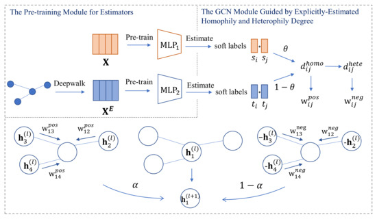
Figure 2.
The schema of GCN-EHHD.
3.2. The Pre-Training Module for Estimators
In order to make full use of the graph information, we pre-train two MLPs by learning from two MLPs which use the node attribute information following [22] and localized structure information independently. We choose Deepwalk [24] to mine localized structure information. Deepwalk [24] applies a group of random walk generators to generate node sequences from a graph. For each node in the graph, the random walk generator takes as the first node to visit, samples uniformly from neighbors of and then designates the sampled neighbor as the next node to visit. The generator repeats the sampling process until the maximum length T of the sequence is reached and the sampled nodes form a sequence in order. Then, Skip-gram [30] is used to generate embeddings for each node from random walk sequences. For each node in a random walk sequence, Skip-gram maximizes the probability of the neighbors that co-occur with the node in a window. It iterates over the random walk set and uses gradient descent to train the embedding of nodes. Let be the learned matrix generated by Deepwalk in graph , and let be the i-th column of . will be used to train an estimator.
Then, we define two MLPs, called MLP and MLP, respectively. The l-th layers of the two MLPs can be defined as:
where and are the original feature vector and embedding vector of node respectively, and are the learnable weight matrices, and are the learnable bias vectors, and is an activation function.
Through MLP estimators, we can obtain the soft labels of all the nodes:
where are the outputs of the last layers of MLP and MLP for node , respectively, and , denote the probabilities that node belongs to class j as estimated by MLP and MLP, respectively.
We pre-train estimators by the nodes with known labels and obtain the optimal parameters of MLP and MLP by minimizing the following two loss functions:
where represents the cross entropy.
After the above pre-training process, we obtain the estimators MLP and MLP, and we will use them to estimate the homophily and heterophily degree of the neighboring nodes.
3.3. The GCN Module Guided by Explicitly Estimated Homophily and Heterophily Degree
For any directly connected nodes and in the graph, we use pre-trained estimators to calculate the homophily degree of these two nodes, which is the estimated probability that two nodes belong to the same category:
We take a weighted sum of the two estimated homophily degrees:
The hyperparameter controls the proportion of original node attribute information and localized structure information used in estimation. Meanwhile, we can obtain the estimated heterophily degree between node pairs, which is the estimated probability that two nodes belong to different categories:
Following the settings in BM-GCN [23], for a graph , we add multiple self-loops to it:
where is the identity matrix, and is the self-loop parameter which is used to control the proportion contributed by the node itself when calculating the weights of messages. We use to denote the set of neighbors of node in the graph. We use a softmax operation to normalize the homophily and heterophily degrees between node and all its neighbors to obtain the weights of positive and negative messages:
Then, we use the above weights to guide the message passing in the graph convolutional layer. The l-th graph convolutional layer in GCN-EHHD can be defined by:
where , is an activation function, , and are all learnable weight matrices, and is the learnable bias vector. The hyperparameter controls the proportion of positive and negative messages in the aggregation of signed messages.
Finally, we can obtain the ultimate prediction of GCN-EHHD by:
where K is the number of the convolutional layers in GCN-EHHD, is the predicted results of GCN-EHHD for node , and is the probability that node belongs to class c.
3.4. Optimization Objective
Similar to the loss function in (5), we can calculate the loss of the GCN module by
When training the GCN module of GCN-EHHD, we fine-tune the estimators at the same time. That is, we add the loss of MLP described in Equation (5), the loss of MLP described in Equation (6) and the loss described in Equation (17) as the final loss:
We will jointly train the MLP module and the GCN module by minimizing the above loss function.
4. Experiments
4.1. Experimental Settings
Datasets. We chose eight widely-adopted datasets. Following [26], we used the homophily ratio to describe the homophily level for a graph. We chose three homophilic graph datasets: Cora, Citeseer and Pubmed [31,32], and five heterophilic graph datasets: Texas, Wisconsin, Squirrel, Chameleon and Cornell [18]. The statistics of these datasets are listed in Table 1, where h represents the homophily ratio of a graph, and represents the average degree of nodes in a graph.

Table 1.
Statistics of datasets.
Baseline Methods. We compared our proposed model with the following baselines: (1) MLP which only uses original node attributes information; (2) Deepwalk [24] which only uses graph topology information; (3) GCN-based models under the assumption of homophily: GCN [1] and GAT [2]; and (4) GCN-based models that deal with heterophilic graphs: MixHop [19], Geom-GCN [18], FAGCN [20], H2GCN [26], HOG-GCN [22] and BM-GCN [23].
Implementation. The baselines MLP and Deepwalk were the same methods with the and in GCN-EHHD, respectively, and the parameter settings and training procedures of baselines MLP and Deepwalk were the same as those of the pre-trained and in GCN-EHHD, respectively. For GCN and GAT, the dimension of hidden layers was set as 64, the number of layers was set as 2, the Adam optimizer [33] was used as optimizer, the learning rate was set as 0.001, and the weight decay was set as 5E-4. The number of attention heads in GAT was set as five. The number of training epochs of GCN and GAT was set as 1600 with the early stopping strategy of 100 patience epochs. For other baselines, the optimal parameters and the training procedures were taken as reported in their original papers. We implemented our proposed GCN-EHHD based on PyTorch [34]. We utilized the Adam optimizer [33] to train the GCN-EHHD. In the process of generating embedding using Deepwalk, the number of random walk generators was set as 80, the maximum length of random walk was set as 10, and the windows size was set as 5. For each dataset, the embedding dimension of was the same as the original features . For both the MLP module and the GCN module, the number of layers was searched in {2, 3}, and the dimension of hidden layer was searched in {32, 64}. The learning rate was set in {0.001, 0.005}, and the weight decay was set in {0.02, 5E-4, 5E-5}. For different datasets, The parameter in Equation (11) for controlling the contribution of self-loops was set in {0, 1, 2}, the hyperparameter in Equation (14) was set in {0, 0.4, 0.5}, and the hyperparameter in Equation (9) was set in {0.1, 0.4, 0.6, 1}. The impact of the parameter and is analyzed in Section 4.4. To train GCN-EHHD, the number of pre-training epochs was set as 400, the number of jointly training epochs was set as 1600 with the early stopping strategy with 100 patience epochs following the training procedure of [23].
4.2. Experimental Results
For all eight datasets, we adopted the test approach of [18] and randomly split the data ten times according to the division ratio 48%/32%/20% to generate the training/validation/test sets. We used the mean accuracy on the test set of the ten splits as the result. We report the experimental results of three homophilic graphs in Table 2, and the results of five heterophilic graphs in Table 3.
Table 2.
Node classification accuracy on homophilic graphs (in % ± Standard Error). The best results are in bold, and the second-best results are underlined.
Table 3.
Node classification accuracy on heterophilic graphs (in % ± Standard Error). The best results are in bold, and the second-best results are underlined.
By inspecting Table 2 and Table 3, we have the following observations. On one hand, for homophilic graphs, the performances of GCN-based models under the homophily assumption were similar to that of GCN-based models tailored for dealing with heterophily. This shows that the emerging methods for tackling heterophily have good compatibility for homophily. For heterophilic graphs, these methods tailored for heterophily significantly outperformed traditional GCNs. On the other hand, for homophilic graphs, our GCN-EHHD outperformed all the baselines on Citeseer and Pubmed and achieved the second best on Cora. For heterophilic graphs, GCN-EHHD outperformed all the baselines on the five datasets. Especially, GCN-EHHD achieved 4.83%, 3.17% and 2.01% improvement on Texas, Squirrel and Cornell, respectively. Therefore, our proposed model can achieve the best or comparable performance on both homophilic and heterophilic graphs.
The accuracies of and of the GCN-EHHD are also meaningful for analyzing the performance of GCN-EHHD. We show the accuracies of pre-trained , and final , after fine-tuning in Table 4. In our experiments, in general, the better the MLPs accuracies were, the better the accuracy of the whole GCN-EHHDwas, especially for the large graph. We discuss the effect of pre-trained estimators in Section 4.4.
Table 4.
Node classification accuracies of and of the GCN-EHHD (in % ± Standard Error).
Next, we discuss the computation complexity and model complexity compared with three representative and competitive models, including FAGCN, HOG-GCN and BM-GCN. To facilitate comparison, we assume that for each model, the dimensions of the input layer, the output layer and all hidden layers are equal and denoted by d. Let K be the number of network layers and L be the number of layers of MLP for pre-training the estimators, let be the number of nodes and be the number of edges in a graph. We also take the time cost and the numbers of parameters of FAGCN, HOG-GCN, BM-GCN and GCN-EHHD when conducting experiments on the Cora datasets as examples. Note that the time cost and the numbers of parameters of the three models for comparison are calculated according to their source code implementation.
The computation complexity of a single layer in GCN-EHHD is ), and they are , , for FAGCN, HOG-GCN and BM-GCN, respectively. Note that for HOG-GCN, BM-GCN and GCN-EHHD, the estimated results are calculated at the beginning of model reasoning and are used at each layer of the model. The coefficients of messages must be calculated at each layer for FAGCN, and the linear transformation of features is only used in the first and the last layers in FAGCN but must be used in each layer in HOG-GCN, BM-GCN and GCN-EHHD. So, the computation time of FAGCN grows with the increase of the number of edges of the graph, and the computation time of HOG-GCN, BM-GCN and GCN-EHHD grows in a square number with the increase of the representation dimension of the hidden layer. In our experiments on the Cora dataset, the time cost of one-pass forward reasoning process in FAGCN, HOG-GCN, BM-GCN and GCN-EHHD were 2.00 ms, 361.03 ms, 1.99 ms and 1.99 ms, respectively. It can be seen that our proposed GCN-EHHD consumes relatively less time.
The complexity of parameters in our GCN-EHHD is , and they are , ) and in FAGCN, HOG-GCN and BM-GCN, respectively. Note that the complexity of parameters in HOG-GCN is able to become ) by modeling the edge weights rather than the homophily degree matrix and overlooking the message passing from high-order neighborhoods. Among these models, the number of parameters in FAGCN is generally the smallest, and the number of parameters in HOG-GCN is generally the largest, since the number of nodes and the number of edges in the graph are generally much larger than the hidden layer dimension of the model. Taking the parameters used in the four models when conducting experiments on the Cora dataset as an example, the numbers of parameters of FAGCN, HOG-GCN, BM-GCN and GCN-EHHD were 92.49 k, 26,154.75 k, 336.46 k and 553.36 k, respectively. It can be seen that, our proposed GCN-EHHD achieves an improvement in the experimental performance without too much increase in the number of parameters.
4.3. Visualization
In order to more visually observe the performance of our proposed model and the compared baselines, we performed the visualization tasks for GCN, FAGCN, BM-GCN and GCN-EHHD on Chameleon that is a heterophilic graph. We extracted the output embedding of the last layer of the four models and used t-SNE [35] to project them to a 2D space. The projected result can be seen in Figure 3 where we can find some meaningful phenomena. First, for GCN, many nodes with different categories are mixed together, which once again shows the defect of GCN for learning tasks on heterophilic graphs. Next, for FAGCN, most nodes with the same category are basically clustered together, but the boundaries between clusters are not obvious. For BM-GCN, the classification result was further improved, but there is still no clear boundary between two clusters (i.e., the blue cluster and the purple cluster) in Figure 3c. Finally, for our proposed GCN-EHHD, the boundaries between clusters are the clearest compared with the other three models. This visualization result once again demonstrates the effectiveness of our proposed model.
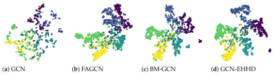
Figure 3.
The visualization of the output embedding of the last layer in GCN, FAGCN, BM-GCN and GCN-EHHD on the Chameleon dataset by t-SNE with nodes colored according to their class labels.
4.4. Ablation Study
In order to explore the role of negative message passing guided by heterophily degree and estimator generated by Deepwalk, we conducted an ablation study. Recall that the hyperparameter in Equation (14) controls the proportion of aggregated positive and negative messages from the neighbors, and the hyperparameter in Equation (9) controls the proportion of node attributes and graph structure information when estimating homophily degree and heterophily degree. We therefore perform an ablation study by comparing different settings of parameters and , and report their effects on the predictive accuracy of node classification tasks.
We chose eleven values of in the interval . When , it amounts to discarding the part of negative message passing and only aggregating positive messages from neighbors. When , the reverse is true. For each setting of , we chose eleven values of ranging from 0 to 1. When , we only used the pre-trained estimator generated based on graph structure information extracted by Deepwalk. When , we only considered node attributes for estimating the homophily and heterophily degree. For each setting of and , we conducted node classification experiments as described in Section 4.2 on the aforementioned eight datasets in Section 4.1 and report the experimental results as given in Figure 4, Figure 5, Figure 6 and Figure 7.
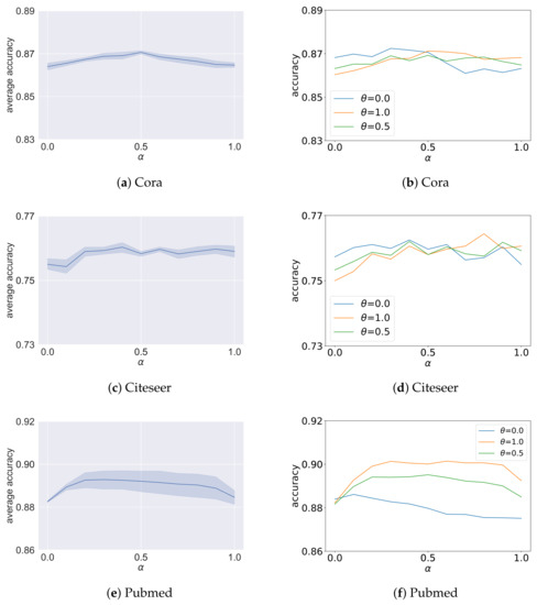
Figure 4.
Analysis results of the ablation study on for homophilic graphs. The x-axis is different settings of . The y-axis of figures on the left shows the average accuracy under eleven different settings of , and the y-axis of figures on the right shows the accuracy for , respectively.
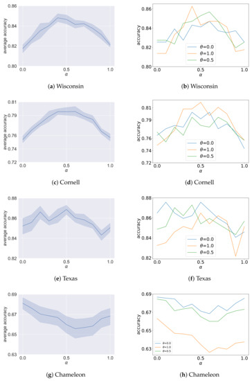
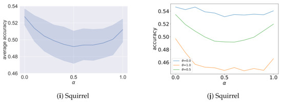
Figure 5.
Analysis results of the ablation study on for heterophilic graphs. The x-axis is different settings of . The y-axis of figures on the left shows the average accuracy under eleven different settings of , and the y-axis of figures on the right shows the accuracy for , respectively.
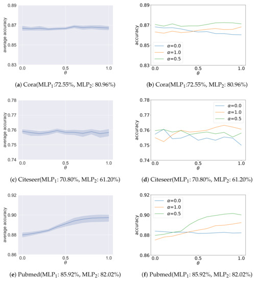
Figure 6.
Analysis results of the ablation study on for homophilic graphs. The x-axis is different settings of . The y-axis of figures on the left shows the average accuracy under eleven different settings of , and the y-axis of figures on the right shows the accuracy for , respectively.
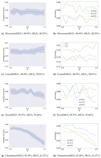
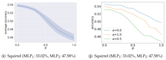
Figure 7.
Analysis results of the ablation study on for heterophilic graphs. The x-axis is different settings of . The y-axis of figures on the left shows the average accuracy under eleven different settings of , and the y-axis of figures on the right shows the accuracy for , respectively.
The analysis results of the ablation study on are shown in Figure 4 and Figure 5. For each sub-figure, the x-axis is different settings of , and under each setting of , the y-axis coordinate value of the figures on the left shows the average accuracy given the aforementioned eleven different settings of , and the y-axis coordinate value of the figures on the right shows the classification accuracy for , respectively. As shown, there are three main situations. For the first situation, the influence of on the model accuracy in average is small for graphs such as Cora, Citeseer and Pubmed. For the second situation, the plots are characterized by sort of “reverse U-shape”, where the accuracy values for and are close to each other, and the best results are obtained in the vicinity of . The analysis results for Wisconsin, Cornell and Texas are this case. In the third situation, the plots for Chameleon and Squirrel are characterized by sort of “U-shape”. When , that is, the negative message passing is cancelled, the performance is not the best in the eight datasets, and in particular is poor on Cornell, Wisconsin and Texas. This validates the effectiveness of negative message passing. For Cora, Citeseer, Pubmed, Wisconsin, Cornell and Texas, when the value of is set to be approximately 0.5, the performance is the best. Consider that the ablated GCN-EHHD models with are similar, so the accuracy for and is close. For Chameleon and Squirrel, the performance is the best when ; that is, we only use negative message passing, and the performance is the worst in the vicinity of . We think the difference is related to the average degree of nodes in graphs. As shown in Table 1, the average degrees of nodes in Chameleon and Squirrel are both much larger than the other datasets. For graphs with a small average degree, the influence of homophilic neighbors and heterophilic neighbors can both play important roles in message passing on heterophilic graphs. This may be the reason why the best performance is obtained in the vicinity of for Wisconsin, Cornell and Texas. Therefore, while for most graphs we can obtain a good performance by mixing positive messages with negative messages, for some heterophilic graphs with large average node degrees, it may be better to keep using negative messages alone.
The analysis results of the ablation study on are shown in Figure 6 and Figure 7. For each sub-figure, the x-axis is different settings of , and under each setting of , the y-axis coordinate value of the figures on the left shows the average accuracy given the aforementioned eleven different settings of . The y-axis coordinate value of the figures on the right shows the classification accuracy for , respectively. In addition, we also annotate each sub-figure with the accuracy of two pre-trained MLPs. As shown, there are three main situations. For the first situation, the better accuracy of GCN-EHHD is obtained for the values of that give more importance to the pre-trained MLP with best performances on graphs such as Chameleon and Squirrel as shown in Figure 7g,h and Figure 7i,j, and Pubmed as shown in Figure 6e and Figure 6f, respectively. These three graphs are relatively large compared with other datasets. In particular, the average degree of nodes in Chameleon and Squirrel is quite large. For the second situation, the influence of on the accuracy of GCN-EHHD is small for graphs such as Cora and Citeseer as shown in Figure 6a,b and Figure 6c,d, respectively. The difference in accuracy between the two pre-trained MLPs used for analyzing Cora and Citeseer is about 10% and not as significant as for other datasets. For the third situation, the accuracy of GCN-EHHD fluctuates with the change of on graphs such as Texas, Cornell and Wisconsin as shown in Figure 7c–f and Figure 7a,b, respectively. The special performance in the third situation may mainly be because the three graphs are all relatively small which causes instability. The results indicate that the pre-trained estimator using Deepwalk is useful in measuring the homophiliy and heterophily degree on some large graphs, especially for those with large node degrees.
5. Conclusions
We proposed a new model called GCN-EHHD in order to better generalize GCN-based methods to deal with heterophilic graphs. In GCN-EHHD, we pre-trained estimators on homophily degree and heterophily degree between neighbouring nodes and leveraged the information to adaptively guide propagation/aggregation of the positive messages and negative messages. Since both node attributes and graph topology matter to the prediction accuracy, we propose applying Deepwalk to extract the structure information of graphs for training an estimator that is combined with the estimator learned from original node attributes to estimate accurate homophily and heterophily degree between node pairs. Our experiments with eight datasets demonstrate the effectiveness of the proposed approach. The proposed new approach achieved state-of-the-art results on three homophilic graphs and outperformed baselines on five heterophilic graphs. Our extensive experiments show that the explicit propagation of signed messages adaptively guided by heterophily degree is important in the message-passing process of heterophilic graphs. The exploration of graph structure information by using Deepwalk turned out to be useful for large heterophilic graphs such as Chameleon and Squirrel, for which the graph topology seemed to play a more decisive role than node attributes as shown by the accuracy of pre-trained estimators. In future work, it would be interesting to explore models other than MLPs to train more effective estimators and study more large graphs with a variety of statistical properties.
Author Contributions
Conceptualization, R.Z. and X.L.; methodology, R.Z. and X.L.; software, R.Z.; validation, X.L.; formal analysis, R.Z. and X.L.; funding acquisition, X.L.; investigation, R.Z.; resources, X.L.; data curation, R.Z. and X.L.; writing—original draft preparation, R.Z. and X.L.; writing—review and editing, R.Z. and X.L.; visualization, R.Z.; supervision, X.L.; project administration, X.L. All authors have read and agreed to the published version of the manuscript.
Funding
This work was supported in part by the Ministry of Science and Technology of China under Grant No. 2018YFC0830400, National Natural Science Foundation of China under Grant No. 61802126.
Institutional Review Board Statement
Not applicable.
Informed Consent Statement
Not applicable.
Data Availability Statement
The data analysed in this study can be accessed at https://github.com/xtyi1997/geom-gcn (accessed on 20 August 2022).
Conflicts of Interest
The authors declare no conflict of interest.
References
- Kipf, T.N.; Welling, M. Semi-supervised classification with graph convolutional networks. In Proceedings of the International Conference on Learning Representations, Toulon, France, 24–26 April 2017. [Google Scholar]
- Veličković, P.; Cucurull, G.; Casanova, A.; Romero, A.; Liò, P.; Bengio, Y. Graph attention networks. In Proceedings of the International Conference on Learning Representations, Vancouver, BC, Canada, 30 April–3 May 2018. [Google Scholar]
- Hamilton, W.; Ying, Z.; Leskovec, J. Inductive representation learning on large graphs. Adv. Neural Inf. Process. Syst. 2017, 30. [Google Scholar]
- Leskovec, K.X.W.H.J.; Jegelka, S. How powerful are graph neural networks? In Proceedings of the International Conference on Learning Representations (ICLR), New Orleans, LA, USA, 6–9 May 2019.
- Wu, Z.; Pan, S.; Chen, F.; Long, G.; Zhang, C.; Philip, S.Y. A comprehensive survey on graph neural networks. IEEE Trans. Neural Netw. Learn. Syst. 2020, 32, 4–24. [Google Scholar] [CrossRef] [PubMed]
- Yao, L.; Mao, C.; Luo, Y. Graph convolutional networks for text classification. In Proceedings of the AAAI Conference on Artificial Intelligence, Honolulu, HI, USA, 27–28 January 2019; Volume 33, pp. 7370–7377. [Google Scholar]
- Marcheggiani, D.; Titov, I. Encoding sentences with graph convolutional networks for semantic role labeling. In Proceedings of the EMNLP, Copenhagen, Denmark, 7–11 September 2017. [Google Scholar]
- Ying, R.; He, R.; Chen, K.; Eksombatchai, P.; Hamilton, W.L.; Leskovec, J. Graph convolutional neural networks for web-scale recommender systems. In Proceedings of the 24th ACM SIGKDD International Conference on Knowledge Discovery & Data Mining, London, UK, 19–23 August 2018; pp. 974–983. [Google Scholar]
- He, X.; Deng, K.; Wang, X.; Li, Y.; Zhang, Y.; Wang, M. Lightgcn: Simplifying and powering graph convolution network for recommendation. In Proceedings of the 43rd International ACM SIGIR Conference on Research and Development in Information Retrieval, Xi’an, China, 25–30 July 2020; pp. 639–648. [Google Scholar]
- Yan, Y.; Zhu, J.; Duda, M.; Solarz, E.; Sripada, C.; Koutra, D. Groupinn: Grouping-based interpretable neural network for classification of limited, noisy brain data. In Proceedings of the 25th ACM SIGKDD International Conference on Knowledge Discovery & Data Mining, Anchorage, AK, USA, 4–8 August 2019; pp. 772–782. [Google Scholar]
- Zheng, X.; Liu, Y.; Pan, S.; Zhang, M.; Jin, D.; Yu, P.S. Graph neural networks for graphs with heterophily: A survey. arXiv 2022, arXiv:2202.07082. [Google Scholar]
- Gilmer, J.; Schoenholz, S.S.; Riley, P.F.; Vinyals, O.; Dahl, G.E. Neural message passing for quantum chemistry. In Proceedings of the International Conference on Machine Learning, Sydney, Australia, 6–11 August 2017; pp. 1263–1272. [Google Scholar]
- Chung, F.R.; Graham, F.C. Spectral Graph Theory; American Mathematical Society: Providence, RI, USA, 1997; Volume 92. [Google Scholar]
- Bruna, J.; Zaremba, W.; Szlam, A.; LeCun, Y. Spectral networks and deep locally connected networks on graphs. In Proceedings of the 2nd International Conference on Learning Representations (ICLR 2014), Banff, AB, Canada, 14–16 April 2014. [Google Scholar]
- Wu, F.; Souza, A.; Zhang, T.; Fifty, C.; Yu, T.; Weinberger, K. Simplifying graph convolutional networks. In Proceedings of the International Conference on Machine Learning, Long Beach, CA, USA, 9–15 June 2019; pp. 6861–6871. [Google Scholar]
- Nt, H.; Maehara, T. Revisiting graph neural networks: All we have is low-pass filters. arXiv 2019, arXiv:1905.09550. [Google Scholar]
- Pandit, S.; Chau, D.H.; Wang, S.; Faloutsos, C. Netprobe: A fast and scalable system for fraud detection in online auction networks. In Proceedings of the 16th international conference on World Wide Web, Banff, AB, Canada, 8–12 May 2007; pp. 201–210. [Google Scholar]
- Pei, H.; Wei, B.; Chang, K.C.C.; Lei, Y.; Yang, B. Geom-gcn: Geometric graph convolutional networks. In Proceedings of the International Conference on Learning Representations, New Orleans, LA, USA, 6–9 May 2019. [Google Scholar]
- Abu-El-Haija, S.; Perozzi, B.; Kapoor, A.; Alipourfard, N.; Lerman, K.; Harutyunyan, H.; Ver Steeg, G.; Galstyan, A. Mixhop: Higher-order graph convolutional architectures via sparsified neighborhood mixing. In Proceedings of the International Conference on Machine Learning, Long Beach, CA, USA, 9–15 June 2019; pp. 21–29. [Google Scholar]
- Bo, D.; Wang, X.; Shi, C.; Shen, H. Beyond low-frequency information in graph convolutional networks. In Proceedings of the AAAI Conference on Artificial Intelligence, Virtual, 2–9 February 2021; Volume 35, pp. 3950–3957. [Google Scholar]
- Shuman, D.I.; Narang, S.K.; Frossard, P.; Ortega, A.; Vandergheynst, P. The emerging field of signal processing on graphs: Extending high-dimensional data analysis to networks and other irregular domains. IEEE Signal Process. Mag. 2013, 30, 83–98. [Google Scholar] [CrossRef]
- Wang, T.; Jin, D.; Wang, R.; He, D.; Huang, Y. Powerful Graph Convolutional Networks with Adaptive Propagation Mechanism for Homophily and Heterophily. In Proceedings of the AAAI Conference on Artificial Intelligence, Virtual, 6–10 November 2022; Volume 36, pp. 4210–4218. [Google Scholar]
- He, D.; Liang, C.; Liu, H.; Wen, M.; Jiao, P.; Feng, Z. Block modeling-guided graph convolutional neural networks. In Proceedings of the AAAI Conference on Artificial Intelligence, Virtual, 6–10 November 2022; Volume 36, pp. 4022–4029. [Google Scholar]
- Perozzi, B.; Al-Rfou, R.; Skiena, S. Deepwalk: Online learning of social representations. In Proceedings of the 20th ACM SIGKDD International Conference on Knowledge Discovery and Data Mining, New York, NY, USA, 24–27 August 2014; pp. 701–710. [Google Scholar]
- Liu, M.; Wang, Z.; Ji, S. Non-local graph neural networks. IEEE Trans. Pattern Anal. Mach. Intell. 2021. [Google Scholar] [CrossRef] [PubMed]
- Zhu, J.; Yan, Y.; Zhao, L.; Heimann, M.; Akoglu, L.; Koutra, D. Beyond homophily in graph neural networks: Current limitations and effective designs. Adv. Neural Inf. Process. Syst. 2020, 33, 7793–7804. [Google Scholar]
- Jin, D.; Yu, Z.; Huo, C.; Wang, R.; Wang, X.; He, D.; Han, J. Universal Graph Convolutional Networks. In Proceedings of the 35th Conference on Neural Information Processing Systems (NeurIPS 2021), online, 6–14 December 2021. [Google Scholar]
- Yan, Y.; Hashemi, M.; Swersky, K.; Yang, Y.; Koutra, D. Two sides of the same coin: Heterophily and oversmoothing in graph convolutional neural networks. arXiv 2021, arXiv:2102.06462. [Google Scholar]
- Zhu, J.; Rossi, R.A.; Rao, A.; Mai, T.; Lipka, N.; Ahmed, N.K.; Koutra, D. Graph neural networks with heterophily. In Proceedings of the AAAI Conference on Artificial Intelligence, Virtual, 2–9 February 2021; Volume 35, pp. 11168–11176. [Google Scholar]
- Mikolov, T.; Chen, K.; Corrado, G.; Dean, J. Efficient estimation of word representations in vector space. arXiv 2013, arXiv:1301.3781. [Google Scholar]
- Sen, P.; Namata, G.; Bilgic, M.; Getoor, L.; Galligher, B.; Eliassi-Rad, T. Collective classification in network data. AI Mag. 2008, 29, 93. [Google Scholar] [CrossRef]
- Namata, G.; London, B.; Getoor, L.; Huang, B.; Edu, U. Query-driven active surveying for collective classification. In Proceedings of the 10th International Workshop on Mining and Learning with Graphs, Scotland, UK, 1 July 2012; Volume 8, p. 1. [Google Scholar]
- Kingma, D.P.; Ba, J. Adam: A Method for Stochastic Optimization. In Proceedings of the ICLR (Poster), San Diego, CA, USA, 7–9 May 2015. [Google Scholar]
- Paszke, A.; Gross, S.; Massa, F.; Lerer, A.; Bradbury, J.; Chanan, G.; Killeen, T.; Lin, Z.; Gimelshein, N.; Antiga, L.; et al. Pytorch: An imperative style, high-performance deep learning library. Adv. Neural Inf. Process. Syst. 2019, 32. [Google Scholar]
- Van der Maaten, L.; Hinton, G. Visualizing data using t-SNE. J. Mach. Learn. Res. 2008, 9, 2579–2605. [Google Scholar]


Publisher’s Note: MDPI stays neutral with regard to jurisdictional claims in published maps and institutional affiliations. |
© 2022 by the authors. Licensee MDPI, Basel, Switzerland. This article is an open access article distributed under the terms and conditions of the Creative Commons Attribution (CC BY) license (https://creativecommons.org/licenses/by/4.0/).