Hyperparameter Tuned Deep Autoencoder Model for Road Classification Model in Intelligent Transportation Systems

Abstract

Unmanned aerial vehicles (UAVs) have significant abilities for automatic detection and mapping of urban surface materials due to their high resolution. It requires a massive quantity of data to understand the ground material properties. In recent days, computer vision based approaches for intelligent transportation systems (ITS) have gained considerable interest among research communities and business people. Road classification using remote sensing images plays a vital role in urban planning. It remains challenging because of scene complexity, fluctuating road structures, and inappropriate illumination circumstances. The design of intelligent models and other machine learning (ML) approaches for road classification has yet to be further explored. In this aspect, this paper presents a metaheuristics optimization with deep autoencoder enabled road classification model (MODAE-RCM). The presented MODAE-RCM technique mainly focuses on the classification of roads into five types, namely wet, ice, rough, dry, and curvy roads. In order to accomplish this, the presented MODAE-RCM technique exploits modified fruit fly optimization (MFFO) with neural architectural search network (NASNet) for feature extraction. In order to classify roads, an interactive search algorithm (ISA) with a DAE model is used. The exploitation of metaheuristic hyperparameter optimizers helps to improve the classification results. The experimental validation of the MODAE-RCM technique was tested by employing a dataset comprising five road types. The simulation analysis highlighted the superior outcomes of the MODAE-RCM approach to other existing techniques.

1. Introduction

In recent times, intelligent transportation systems (ITS) using unmanned aerial vehicles (UAV) have become essential. A set of comprehensive data regarding road networks is considered to be one of the transportation features which helps in planning and assessing transportation [1]. Retrieval of road data such as road surface materials and pavement type condition was one important problem in urban areas. This can be performed by remote sensing (RS) or conventional surveying [2]. The traditional method requires huge labour and consumes more time. Hyperspectral image, otherwise called imaging spectrometry, can be defined as acquiring data in several narrow, contiguous spectral bands. It offers detailed data compared to other RS methods [3]. Various chemical materials, such as gravel and asphalt, are extracted on a detailed level through hyperspectral images by their respective physical properties (reflectivity, absorption, albedo, and many more). This feature will be useful to discriminate and extract objects of cities, particularly those having the same spectral property [4]. Road surface materials are detected through hyperspectral images, incurring less cost than field surveying. Many existing approaches to map roads can be either semi-automatic or manual [5]. However, such techniques will be expensive and consume more time. Particularly, they might include more field work and clarification of aerial images, through which limited data is obtained. Hyperspectral data contains substantial potentiality relating to automatic detection of road surface materials [6]. However, no standard technique to map road surfaces or find the state of road surface resources has existed until now. Many existing techniques were first formulated for mineral detection. Therefore, it will be difficult to leverage such techniques in detecting road surface materials, because of the difference in such resources in the case of roads in smaller regions [7].

General road categories include ice, dry, rough, and curvy road surfaces. Classification of these road forms will be a fascinating issue. In this context, several image processing methods are used for assisting smart vehicles and for classifying various road categories [8]. However, the road image quality is affected through dynamic weather, illumination variation, and blurring. Progressive approaches, such as deep learning (DL), are helpful for observing the challenging atmosphere by a computer vision (CV) technique, and might help smart vehicles to modify their driving performance depending on the road type [9]. Driving performance mainly disturbs people near road regions, most often if a road has a medium amount of traffic. It is unrealistic to assess the condition of each road which a smart vehicle could approach [10]. There are massive variables that must be considered when handling such vehicles, including a difference in heavy traffic, varying meteorological conditions, and road conditions.

This paper presents a metaheuristics optimization with a deep autoencoder enabled road classification model (MODAE-RCM). The presented MODAE-RCM technique mainly focuses on the classification of roads into five types, namely wet, ice, rough, dry, and curvy roads. For accomplishing this, the presented MODAE-RCM technique exploits modified fruit fly optimization (MFFO) with a neural architectural search network (NASNet) for feature extraction. In order to classify roads, an interactive search algorithm (ISA) with the deep autoencoder enabled model (DAE) is used. The exploitation of metaheuristic hyperparameter optimizers helps to considerably improve the classification results. The experimental validation of the MODAE-RCM technique was tested using a dataset comprising five road types.

2. Literature Review

Alshehhi et al. [11] presented a single patch-related convolutional neural network (CNN) structure for the extraction of buildings and roads from high-resolution remote sensing (RS) datasets. Low-level features of buildings and roads (i.e., compactness and asymmetry) in nearby areas were compiled with CNN attributes at the time of post-processing phase for the purpose of enhancing the act. Lourenço et al. [12] recognized the potential of the object-based image analysis (OBIA) method for mapping numerous invasive plant species across roads, utilizing high spatial resolution images. Secondly, the author repeated the earlier classification and segmentation stages on the fifteen masked images of vegetated regions.

Zhang et al. [13] modeled a new stagewise domain adaptation method, termed Road domain adaptation (RoadDA), for addressing data structure (DS) problems in this domain. In the initial phase, RoadDA would adapt the targeted domain attributes for aligning the source ones through Generative Adversarial Network (GAN)-related interdomain adaptation. Particularly, feature pyramid fusion modules are formulated in order to evade data loss of thin and long roads, and to study discriminatory and robust attributes. In addition, to solve intradomain discrepancy in the targeted field, in the next phase, the author modeled an adversarial self-trained technique. Chen et al. [14] devised an Adaboost-like End-To-End Multiple Lightweight U-Nets method (AEML U-Nets) for the purpose of extracting roads. The authors in [15] devised a compiled technique merging classification and segmentation techniques with linked component analysis, for the purpose of extracting road class out of orthophoto imageries. This modeled approach was threefold. Firstly, a multiresolution segmenting technique has been implemented for image segmentation. After, the main classification techniques like Vector Machines (SVM), Decision Tree (DT), and k-Nearest Neighbor (KNN) are applied on the basis of textural, spectral, and geometric data. The acquired outcomes are classified into 2 classes, namely, non-road and road.

Ding et al. [16] modeled Non-Local Feature Search Networks (NFSNets) that could enhance the segmentation precision of RS imageries of roads and buildings, and attain precise urban planning. It could efficiently minimize the big area misclassifications of road and building discontinuation in the segmenting procedure. The Global Feature Refinement (GFR) components were presented for the purpose of integrating the features derived from the SAFT module and backbone network. It improvises the semantic data belonging to the feature map and gains a more detailed segmenting outcome. Dewangan et al. [17] modeled a CNN-related road classification network (RCNet) for the precise categorization of road surfaces. This process involves five categories of road surfaces, namely rough, curvy, ice, dry, and wet roads. The simulation outcomes show the performance of this presented RCNet in different optimizer approaches. The standard performance assessment measures were employed for the purpose of testing and validating this presented technique on the Oxford RobotCar data.

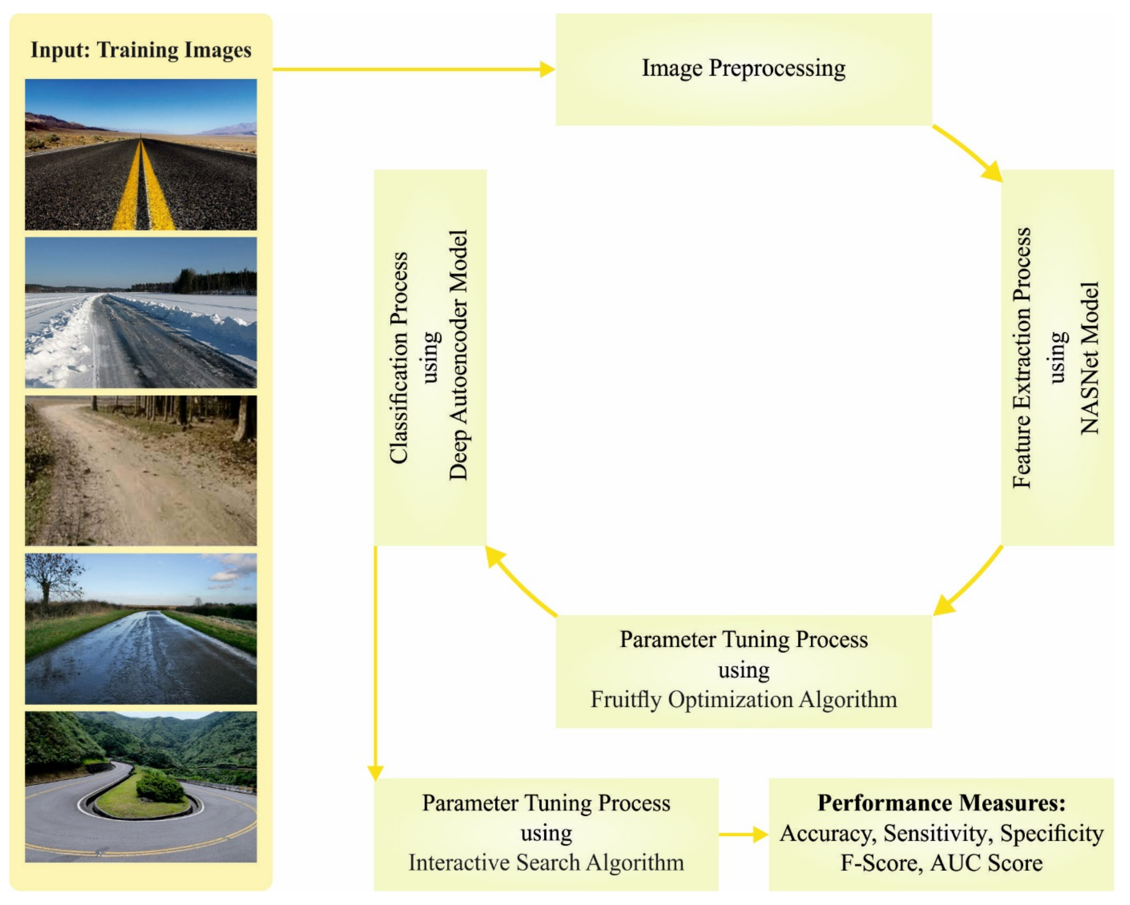
3. Materials and Methods

In this study, a new MODAE-RCM method was formulated for accurate and automated road classification. The presented MODAE-RCM technique mainly focuses on the classification of roads into five types, namely wet, ice, rough, dry, and curvy roads. It encompasses a series of processes, namely MFFO with NASNet feature extraction, DAE classification, and ISA hyperparameter optimizer. Figure 1 illustrates the workflow of MODAE-RCM system.

3.1. Feature Extraction

The presented MODAE-RCM technique exploited the MFFO with the NASNet model for feature extraction. The NASNet Mobile technique was a recently accomplished DL method with 5,326,716 variables, which will exhibit maximum reliability. The NASNet structure has a building block, and a group of blocks was jointly integrated for cell formation. The search space involved in the NASNet was the factorization of a network to cells, which was divided into blocks. The kind of blocks and cell count are not predetermined [18]. However, they must be improved for the dataset which is chosen. The probable function of the block includes max pooling, separable convolution, average pooling, identity map, convolution, and many more. The blocks are capable of mapping two inputs into output featured mapping. The network growth can be focused on three attributes, namely the amount of cells that are stacked (N), the count of filters from the primary layer (F), and the cell infrastructure.

In order to regulate the hyperparameters of the NASNet method, the MFFO algorithm was applied to it. Generally, FFO is easier to design; however, it suffers from local optimal problems [19]. The flight direction and distance of osphresis foraging are not regular, and blind flight can decrease the searching act of the FFO method. Therefore, the MFFO technique was designed by the use of Levi flight into osphresis foraging for the purpose of adjusting the direction and distance of the FFO algorithm. Levi flight is a type of walking stage among short distance searches and, sporadically, long distance walks. Therefore, it could raise population diversity and extend the searching area, which causes the FFO algorithm to escape from local optima problems and decrease the possibility of earlier convergence. In addition, a condition probability $P_a$ is defined as vision foraging for the challenging optimum location that can be defined in order to enhance the searching accuracy of the FFO algorithm. The algorithmic process of the MFFO algorithm is defined as the following:

Step 1: initializing parameters. Fix maximum number of iterations as $G_{\max }$, the FF swarm size as $N$, and FF location $X_{i,0},$ $Y_{i,0}$ and optimum position $X_{b,0},$ $Y_{b,0}$ arbitrarily in the interval of $\left[0, 1\right].$

Step 2: upgrade the location of the FF by the Levi flight:

$$X_{i,G}=X_{b,G-1}\pm \left(X_{i,G-1}-X_{b,G-1}\right)\otimes L\left(\beta \right), i=1,2,\dots n$$

(1)

$$Y_{i,G}=Y_{b,G-1}\pm \left(Y_{i,G-1}-Y_{b,G-1}\right)\otimes L\left(\beta \right), i=1,2,\dots n$$

Step 3: execute the FFO process.

Step 4: produce an arbitrary number $P_t$.

Step 5: compute the difference between optimum solutions $X{b}_{estindx,G},$ $Y_{estindx,G}$ and the worst solution $X_{worstindx,G}$ and $Y_{worstindx,G}$ of the population.

[worstSmell worstindex] $=\max \left(F_{i,G}\right)$

$$X_{b,G}=X_{bestindex,G}-\frac{G_{\max }}{G}\log \left(\frac{G}{G_{\max } }\right)\left(X_{bestindex, G}-X_{worstindex, G}\right)$$

(2)

$$Y_{b,G}=Y_{bestindex,G}-\frac{G_{\max }}{G} \log \left(\frac{G}{G_{\max } }\right)\left(Y_{bestindex, G}-X_{worstindex, G}\right)$$

Step 6: perform optimization and reiterate steps 2–4 to determine if smell concentration is superior to earlier. Then, the process is terminated upon reaching maximum accuracy or fixed number of iterations $G_{\max }$.

The MFFO algorithm will derive a fitness function (FF) for obtaining enhanced classifier outcomes. It would determine a positive value for denoting a superior outcome of candidate solutions. In this work, the reduced classifier error rate will be denoted as the FF, as given in Equation (3).

$$\begin{gathered} fitness\left(x_i\right)=ClassifierErrorRate\left(x_i\right) \\ =\frac{number of misclassified samples}{Total number of samples}\ast 100 \end{gathered}$$

(3)

3.2. Road Classification Using DAE

At this stage, the DAE classifier is applied for classification process. DAE is an Auto-Encoder (AE) with one or more hidden layers (HL) [20]. The addition of HLs from a DAE permits the AE to learn further difficult paradigms of mathematical data. For an AE having a single HL, the procedure of mapping an input layer to the HL was the encoder stage. The mapping of the HL to the output layer is the decoder stage. During the DAE with several HLs, encoding and decoding pairs are added. The DAE infrastructure comprises five HLs (collected of three encoding and decoding pairs). The DAE phase starts with the stage in which the primary encoding $\left(E1\right)$ encrypts input $X$, the secondary encoding $\left(E2\right)$ encrypts the outcome in $E1,$ and the tertiary encoding $\left(E3\right)$ encrypts the outcome in $E2$. The encoder stage is expressed on the middle layer as $Z=E3\left(E2\left(E1\left(X\right)\right)\right)$.

In a single HL, the AE vector encoded $h$ is written as $h=$ $f\left(W.X+b\right)$, whereas $W$ stands for the weighted matrix, $b$ denotes the bias vector, and $X$ indicates the input vector. The vector encoder’s purpose in forwarding propagation to HL 1 develops in Equation (4).

$$h^{\left(l+1\right)}=f\left(W^{\left(l\right)}.h^{\left(l\right)}+b^{\left(l\right)}\right),$$

(4)

so that in the encoder stage, all of the layers are expressed as $E1=f\left(W^{\left(1\right)}.X+b^{\left(1\right)}\right);E2=f\left(W^{\left(2\right)}\right).E1+b^{\left(2\right)}$; and $Z=E3=f\left(W^{\left(3\right)}\right).E2+b^{\left(3\right)}.$ The decoder stage was applied in the opposite way to the encoder stage: a primary decoder was the last to decode. The last reconstruction stage of the decoded vector outcome was $\widehat{X}=D1\left(D2\left(D3\left(E3\left(E2\left(E1\left(X\right)\right)\right)\right)\right)\right)$. For an AE with single HL, $\widehat{X}=f\left(W^T.h+b^{\prime }\right)$, the decoder function to DAE develops as: $D3=f((W^{\left(3\right)}{)}^T.Z+b^{{(3)}^{\prime }});D2=f((W^{\left(2\right)}{)}^T.D3+b^{{(2)}^{\prime }});\widehat{X}=D1=f((W^{\left(1\right)}{)}^T.D2+b^{{(1)}^{\prime }})$, whereas $f$ refers to the node activation function (AF) utilized on all the layers. The AF $f$ on NN neurons is a mathematical purpose carried out to the resultant signal utilized for enabling or disabling neurons. The AF maps resultant values into a chosen range, between $-1$ and 1 or $0$ and 1 (depending upon the AF utilized). Figure 2 depicts the infrastructure of AE.

The cost function of DAE was the distance function between input and reconstructing $\widehat{X}.$ Cost, also called loss, was computed with Mean Square Error (MSE) loss to AF:

$$J\left(w, b, x^j,\widehat{x}\right)=\frac{1}{2}\Vert x^i-\widehat{x}{\Vert }^2$$

(5)

The input data were normalized to between $\mathrm{zero}$ and one; afterward, the reconstruction procedure on the resultant layer was conducted with non-linear sigmoid functions. In order to input, either the binary number or the input with a range between $\mathrm{zero}$ and one was utilized for binary cross-entropy as loss functions $\left[4y,n8\right]$. To the entire train of $m$ data, $\left(w, b\right)=$ $\frac{1}{m}{{\displaystyle \sum }}_{i=1}^{m}J\left(w, b, x^i,{\widehat{x}}^{\mathrm{i}}\right)$. The minimum loss value was computed utilizing the subsequent formula:

$$J\left(w, b\right)=\frac{1}{m}{\displaystyle \sum }_{i=1}^m[x^i \log ({\widehat{x}}^{\mathrm{i}})+(1-x^i) \log \left(1-\widehat{x}\right)]$$

(6)

Back-propagation (BP) upgraded the biases and weight values of all the nodes from all the layers, for the purpose of decreasing the cost. An optimum cost of the most minimum loss value was nearly 0. Afterward, in the AE trained procedure, the data on the bottleneck (Z) layer was a representation of data from the low dimensional encoder procedure. The encoder infrastructure (Z) was put forward as input to a DNN technique called transfer learning (TL). In TL, the $Z$-encoder infrastructure transmitted to AE and the biases and weights values were classified.

3.3. Hyperparameter Tuning

Finally, the ISA technique was exploited for the optimal hyperparameter optimizer. The ISA technique is gradient-free, and population-based search technique that was used was established by Mortazavi et al. [21]. All the agents from the ISA technique which were dependent upon their tendency factor $\left({\tau }_i\right)$ utilized both track and interact stages for the purpose of updating their place. During the tracking stage, the agent searched the vicinity of places spotted by particular agents as the optimum agent $\left(X^G\right)$, the weighting agent $\left(X^W\right)$, and the optimum place of arbitrary agents kept in the preceding optimum matrix $\left(X^P\right)$. During the interact stage, the agent upgraded its place, depending upon pairwise data shared with other arbitrary agents. The ISA technique’s mathematical equation was:

if ${\tau }_i\ge 0.3 \left[Tracking phase\right]$:

$$t+1={\omega }_0\cdot {}_{ }{}^{t}V{}_i+{\varphi }_1\cdot \left({}_{ }{}^{t}X{}_i^P-{}_{ }{}^{t}X{}_j\right)+{\varphi }_2\left({}_{ }{}^{t}X{}^G-{}_{ }{}^{t}X{}_i^P\right)+{\varphi }_3\left({}_{ }{}^{t}X{}^W-{}_{ }{}^{t}X{}_i\right)$$

(7)

if ${\tau }_i<0.3$ $\left[Interacting phase\right]$:

$${}_{ }{}^{t+1}V{}_i={\varphi }_4\left({}_{ }{}^{t}X{}_j-{}_{ }{}^{t}X{}_j\right)$$

(8)

Upgrade equation:

$${}_{ }{}^{t+1}X{}_i={}_{ }{}^{t}X{}_i{+}^{t+1}{V}_i$$

(9)

where the upper left superscripts “t + 1” and “t” denote upgrade and present states of variables, correspondingly; ${\tau }_i$ denotes the tendency factor arbitrarily selected in the range between zero and one; $0_0$ signifies the coefficient that is always obtained as 0.4. ${\varphi }_1$, ${\varphi }_2$, and ${\varphi }_3$ demonstrate coefficients of accelerations which were picked arbitrarily in the range of zero and one; $t_{X^P}$,$t_X$, and $t_{X}G$ represent the agent arbitrarily selected from the agent which kept the previous optimum places, the present agent, and the optimum agents [22]. In addition, $X^W$ refers to the weighting agent, determined as the weight average of every population, and the mathematical equation is given below.

$$X^W={\displaystyle \sum }_{i=1}^{PS}\overline{c}{X}_i^P$$

whereas,

$$\overline{c}=\left(\frac{{\widehat{c}}_i^w}{{{\displaystyle \sum }}_{i=1}^{PS}{\widehat{c}}_i^w}\right)$$

(10)

and

$${\widehat{c}}_i^w=\frac{\underset{i\le k\le PS}{\max }\left(f\left(X_k^P\right)\right)-f\left(X_i^P\right)}{ \max \left(f\left(X_k^P\right)\right)-\underset{i\le k\le PS}{\min }\left(f\left(X_k^P\right)\right)+\mu },i=1,2,\dots ,PS$$

According to this design, $PS$ defines the population size, and $f$ returns the main function value to select agents. Moreover, $\mu$ refers to the smaller positive number for avoiding probable division by zero conditions, and is obtained as 1 × 10⁻⁵.

4. Performance Evaluation

In this section, the road classification performance of the MODAE-RCM method is investigated, utilizing a dataset which comprises 12,500 samples with five types of roads, as depicted in

Table 1. Dataset details.

Class	No. of Samples
Dry	2500
Ice	2500
Rough	2500
Wet	2500
Curvy	2500
Total No. of Samples	12,500

. Figure 3 demonstrates some sample images.

The confusion matrices provided by the MODAE-RCM method on the road classification process are portrayed in Figure 4. The figure highlighted in the MODAE-RCM method has categorized all the types of roads accurately.

Table 2. Road classification outcomes of the MODAE-RCM system with varying classes under the entire database.

Entire Dataset
Class	Accuracy	Sensitivity	Specificity	F-Score	AUC Score
Dry	99.22	98.20	99.48	98.06	98.84
Ice	99.61	98.80	99.81	99.02	99.30
Rough	99.50	98.76	99.68	98.74	99.22
Wet	98.97	96.64	99.55	97.40	98.09
Curvy	99.17	98.76	99.27	97.94	99.02
Average	99.29	98.23	99.56	98.23	98.89

and Figure 5 represent the overall road classification outcomes of the MODAE-RCM approach on the entire dataset. The outcomes reported the MODAE-RCM model has proficiently recognized all of the five distinct kinds of roads on the applied input images. It can be noticed that the MODAE-RCM model has offered an average $acc{u}_y$ of 99.29%, $sen{s}_y$ of 98.23%, $spe{c}_y$ of 99.56%, $F_{score}$ of 98.23%, and $AU{C}_{score}$ of 98.89%.

Table 3. Road classification outcomes of the MODAE-RCM system with varying classes under 70% of the TR database.

Training Phase (70%)
Class	Accuracy	Sensitivity	Specificity	F-Score	AUC Score
Dry	99.21	98.02	99.51	98.05	98.77
Ice	99.59	98.75	99.80	98.97	99.27
Rough	99.46	98.57	99.69	98.65	99.13
Wet	99.01	97.01	99.50	97.49	98.26
Curvy	99.19	98.80	99.29	97.98	99.04
Average	99.29	98.23	99.56	98.23	98.89

and Figure 6 signify the overall road classification outcomes of the MODAE-RCM method on 70% of the TR database. These results indicate that the MODAE-RCM approach has proficiently recognized all of the five distinct kinds of roads in the applied input images. It is noted that the MODAE-RCM approach has presented an average $acc{u}_y$ of 99.29%, $sen{s}_y$ of 98.23%, $spe{c}_y$ of 99.56%, $F_{score}$ of 98.23%, and $AU{C}_{score}$ of 98.89%.

Table 4. Road classification outcomes of the MODAE-RCM system with varying classes under 30% of the TS database.

Testing Phase (30%)
Class	Accuracy	Sensitivity	Specificity	F-Score	AUC Score
Dry	99.25	98.64	99.40	98.10	99.02
Ice	99.65	98.93	99.83	99.13	99.38
Rough	99.57	99.21	99.67	98.94	99.44
Wet	98.88	95.78	99.67	97.19	97.72
Curvy	99.12	98.68	99.23	97.84	98.96
Average	99.30	98.25	99.56	98.24	98.90

and Figure 7 portray the overall road classification outcomes of the MODAE-RCM approach on 30% of the TS database. These outcomes indicate that the MODAE-RCM method has proficiently recognized all of the five distinct kinds of roads on the applied input images. It is noted that the MODAE-RCM approach has rendered an average $acc{u}_y$ of 99.30%, $sen{s}_y$ of 98.25%, $spe{c}_y$ of 99.56%, $F_{score}$ of 98.24%, and $AU{C}_{score}$ of 98.90%.

The training accuracy (TRA) and validation accuracy (VLA) gained by the MODAE-RCM technique under the test database are exemplified in Figure 8. The experimental result denotes that the MODAE-RCM method has reached maximal values of TRA and VLA. Principally, the VLA is greater than the TRA.

The training loss (TRL) and validation loss (VLL) reached by the MODAE-RCM method under the test database are established in Figure 9. The simulation outcome denotes that the MODAE-RCM system has established the lowest values of TRL and VLL. Specifically, the VLL is lesser than the TRL.

A clear precision-recall inspection of the MODAE-RCM technique under the test database is represented in Figure 10. The figure denotes that the MODAE-RCM approach has resulted in enhanced values of precision-recall values in every class label.

Table 5. Comparative analysis of the MODAE-RCM system and other approaches.

Methods	Accuracy	Sensitivity	Specificity	F1-Score
MODAE-RCM	99.30	98.25	99.56	98.24
SGD	74.11	73.46	93.46	71.13
RMSProp	97.65	97.51	99.15	97.28
Adagrad	79.99	80.51	95.07	80.86
Adam	98.62	98.09	98.57	97.89
Adadelta	71.37	71.39	92.51	71.51
Adamax	95.39	96.27	98.59	95.87

provides the overall road classification performance of the MODAE-RCM model with other existing models [17].

Figure 11 reports a brief $acc{u}_y$ examination of the MODAE-RCM with compared approaches. The figure represents that the SGD, Adagrad, and Adadelta models have reported lower classifier results. The RMSProp and Adamax models have shown reasonable $acc{u}_y$ values. Although Adam attempted to gain considerable $acc{u}_y$ of 98.62%, the MODAE-RCM model has accomplished a maximum $acc{u}_y$ of 99.30%.

Figure 12 reports a brief $sen{s}_y$ investigation of the MODAE-RCM with compared approaches. The figure represents that the SGD, Adagrad, and Adadelta models have reported lower classifier results. The RMSProp and Adamax methods also exposed reasonable $sen{s}_y$ values. Although Adam attempted to gain considerable $sen{s}_y$ of 98.09%, the MODAE-RCM method has accomplished a maximum $sen{s}_y$ of 98.25%.

Figure 13 portrays a brief $spe{c}_y$ inspection of the MODAE-RCM system with compared approaches. The figure signifies that the SGD, Adagrad, and Adadelta models have reported lower classifier results. The Adam and Adamax approaches have also revealed reasonable $spe{c}_y$ values. Although the RMSProp attempted to gain a considerable $spe{c}_y$ of 99.15%, the MODAE-RCM method has established a maximum $spe{c}_y$ of 99.56%.

Figure 14 reports a brief $F_{score}$ inspection of the MODAE-RCM system with compared approaches. The figure denotes that the SGD, Adagrad, and Adadelta techniques have reported lower classifier results. The RMSProp and Adamax models have also displayed reasonable $F_{score}$ values. Although Adam attempted to obtain a considerable $F_{score}$ of 97.89%, the MODAE-RCM method has established a maximum $spe{c}_y$ of 98.24%.

After examining the aforementioned results, it was assured that the MODAE-RCM approach has reached maximum road classification performance.

5. Conclusions

In this study, a novel MODAE-RCM algorithm was formulated for accurate and automated road classification. The presented MODAE-RCM technique mainly focuses on the classification of roads into five types, namely wet, ice, rough, dry, and curvy roads. For accomplishing this, the presented MODAE-RCM technique exploited the MFFO with the NASNet model for feature extraction. Finally, the ISA-DAE classifier is applied for the classification process. The exploitation of metaheuristic hyperparameter optimizers helps to improve the classification results. The experimental validation of the MODAE-RCM technique is tested by utilizing a dataset comprising five road types. The simulation analysis pointed out the superior outcomes of the MODAE-RCM technique to other existing techniques. In the future, the performance of the MODAE-RCM approach can be further boosted via hybrid DL models.

References

1. Wang, W.; Yang, N.; Zhang, Y.; Wang, F.; Cao, T.; Eklund, P. A review of road extraction from remote sensing images. J. Traffic Transp. Eng. 2016, 3, 271–282. [Google Scholar] [CrossRef] [Green Version]
2. Kahraman, I.; Karas, I.R.; Akay, A.E. Road extraction techniques from remote sensing images: A review. In Proceedings of the International Conference on Geomatic & Geospatial Technology (Ggt 2018): Geospatial And Disaster Risk Management; Copernicus Gesellschaft Mbh; UTM: Kuala Lumpur, Malaysia, 2018. [Google Scholar]
3. Abdollahi, A.; Pradhan, B.; Shukla, N.; Chakraborty, S.; Alamri, A. Deep learning approaches applied to remote sensing datasets for road extraction: A state-of-the-art review. Remote Sens. 2020, 12, 1444. [Google Scholar] [CrossRef]
4. Gao, L.; Song, W.; Dai, J.; Chen, Y. Road extraction from high-resolution remote sensing imagery using refined deep residual convolutional neural network. Remote Sens. 2019, 11, 552. [Google Scholar] [CrossRef] [Green Version]
5. Karimzadeh, S.; Matsuoka, M. Development of nationwide road quality map: Remote sensing meets field sensing. Sensors 2021, 21, 2251. [Google Scholar] [CrossRef] [PubMed]
6. Al-Qarafi, A.; Alrowais, F.; Alotaibi, S.; Nemri, N.; Al-Wesabi, F.N.; Al Duhayyim, M.; Marzouk, R.; Othma, M.; Al-Shabi, M. Optimal machine learning based privacy preserving blockchain assisted internet of things with smart cities environment. Appl. Sci. 2022, 12, 5893. [Google Scholar] [CrossRef]
7. Xu, Y.; Xie, Z.; Feng, Y.; Chen, Z. Road extraction from high-resolution remote sensing imagery using deep learning. Remote Sens. 2018, 10, 1461. [Google Scholar] [CrossRef] [Green Version]
8. Jia, J.; Sun, H.; Jiang, C.; Karila, K.; Karjalainen, M.; Ahokas, E.; Khoramshahi, E.; Hu, P.; Chen, C.; Xue, T.; et al. Review on active and passive remote sensing techniques for road extraction. Remote Sens. 2021, 13, 4235. [Google Scholar] [CrossRef]
9. Chen, Z.; Deng, L.; Luo, Y.; Li, D.; Junior, J.M.; Gonçalves, W.N.; Nurunnabi, A.A.M.; Li, J.; Wang, C.; Li, D. Road extraction in remote sensing data: A survey. Int. J. Appl. Earth Obs. Geoinf. 2022, 112, 102833. [Google Scholar] [CrossRef]
10. Shao, Z.; Zhou, Z.; Huang, X.; Zhang, Y. MRENet: Simultaneous extraction of road surface and road centerline in complex urban scenes from very high-resolution images. Remote Sens. 2021, 13, 239. [Google Scholar] [CrossRef]
11. Alshehhi, R.; Marpu, P.R.; Woon, W.L.; Dalla Mura, M. Simultaneous extraction of roads and buildings in remote sensing imagery with convolutional neural networks. ISPRS J. Photogramm. Remote Sens. 2017, 130, 139–149. [Google Scholar] [CrossRef]
12. Lourenço, P.; Teodoro, A.C.; Gonçalves, J.A.; Honrado, J.P.; Cunha, M.; Sillero, N. Assessing the performance of different OBIA software approaches for mapping invasive alien plants along roads with remote sensing data. Int. J. Appl. Earth Obs. Geoinf. 2021, 95, 102263. [Google Scholar] [CrossRef]
13. Zhang, L.; Lan, M.; Zhang, J.; Tao, D. Stagewise unsupervised domain adaptation with adversarial self-training for road segmentation of remote-sensing images. IEEE Trans. Geosci. Remote Sens. 2021, 60, 1–13. [Google Scholar] [CrossRef]
14. Chen, Z.; Wang, C.; Li, J.; Fan, W.; Du, J.; Zhong, B. Adaboost-like End-to-End multiple lightweight U-nets for road extraction from optical remote sensing images. Int. J. Appl. Earth Obs. Geoinf. 2021, 100, 102341. [Google Scholar] [CrossRef]
15. Abdollahi, A.; Pradhan, B. Integrated technique of segmentation and classification methods with connected components analysis for road extraction from orthophoto images. Expert Syst. Appl. 2021, 176, 114908. [Google Scholar] [CrossRef]
16. Ding, C.; Weng, L.; Xia, M.; Lin, H. Non-local feature search network for building and road segmentation of remote sensing image. ISPRS Int. J. Geo-Inf. 2021, 10, 245. [Google Scholar] [CrossRef]
17. Dewangan, D.K.; Sahu, S.P. RCNet: Road classification convolutional neural networks for intelligent vehicle system. Intell. Serv. Robot. 2021, 14, 199–214. [Google Scholar] [CrossRef]
18. Falconí, L.G.; Pérez, M.; Aguilar, W.G. Transfer learning in breast mammogram abnormalities classification with mobilenet and nasnet. In Proceedings of the 2019 International Conference on Systems, Signals and Image Processing (IWSSIP), Osijek, Croatia, 5–7 June 2019; pp. 109–114. [Google Scholar]
19. Hu, G.; Xu, Z.; Wang, G.; Zeng, B.; Liu, Y.; Lei, Y. Forecasting energy consumption of long-distance oil products pipeline based on improved fruit fly optimization algorithm and support vector regression. Energy 2021, 224, 120153. [Google Scholar] [CrossRef]
20. Kunang, Y.N.; Nurmaini, S.; Stiawan, D.; Suprapto, B.Y. Attack classification of an intrusion detection system using deep learning and hyperparameter optimization. J. Inf. Secur. Appl. 2021, 58, 102804. [Google Scholar] [CrossRef]
21. Mortazavi, A.; Toğan, V.; Nuhoğlu, A. Interactive search algorithm: A new hybrid metaheuristic optimization algorithm. Eng. Appl. Artif. Intell. 2018, 71, 275–292. [Google Scholar] [CrossRef]
22. Mortazavi, A. Bayesian interactive search algorithm: A new probabilistic swarm intelligence tested on mathematical and structural optimization problems. Adv. Eng. Softw. 2021, 155, 102994. [Google Scholar] [CrossRef]
Figure 1. Workflow of MODAE-RCM system.
Applsci 12 10605 g001
Figure 2. Structure of AE.
Applsci 12 10605 g002
Figure 3. Sample images.
Applsci 12 10605 g003
Figure 4. Confusion matrices of MODAE-RCM system: (a) entire database, (b) 70% of time series database (TR) database, and (c) 30% of time series (TS) database.
Applsci 12 10605 g004
Figure 5. Road classification outcomes of the MODAE-RCM system under the entire database.
Applsci 12 10605 g005
Figure 6. Road classification outcomes of the MODAE-RCM system under 70% of the TR database.
Applsci 12 10605 g006
Figure 7. Road classification outcomes of MODAE-RCM system under 30% of TS database.
Applsci 12 10605 g007
Figure 8. TRA and VLA analysis of the MODAE-RCM system.
Applsci 12 10605 g008
Figure 9. TRL and VLL analysis of the MODAE-RCM system.
Applsci 12 10605 g009
Figure 10. Precision-recall analysis of the MODAE-RCM system.
Applsci 12 10605 g010
Figure 11. A c c u y analysis of the MODAE-RCM system and other approaches.
Applsci 12 10605 g011
Figure 12. S e n s y analysis of MODAE-RCM system and other approaches.
Applsci 12 10605 g012
Figure 13. S p e c y analysis of the MODAE-RCM system and other approaches.
Applsci 12 10605 g013
Figure 14. F 1 s c o r e analysis of the MODAE-RCM system and other approaches.
Applsci 12 10605 g014