Article

Spatial Heterogeneity of Excess Lung Fluid in Cystic Fibrosis: Generalized, Localized Diffuse, and Localized Presentations

by
Ashley V. Schwartz
1,2,†,
Amanda N. Lee
1,2,†,
Rebecca J. Theilmann
3 and
Uduak Z. George
2,*
1
Computational Science Research Center, San Diego State University, San Diego, CA 92182, USA
2
Department of Mathematics and Statistics, San Diego State University, San Diego, CA 92182, USA
3
Department of Radiology, University of California, San Diego, CA 92093, USA
*
Author to whom correspondence should be addressed.
These authors contributed equally to this work.
Appl. Sci. 2022, 12(20), 10647; https://doi.org/10.3390/app122010647
Submission received: 8 September 2022 / Revised: 15 October 2022 / Accepted: 15 October 2022 / Published: 21 October 2022
(This article belongs to the Special Issue Image Processing Techniques for Biomedical Applications II)

Abstract

:
Magnetic resonance (MR) imaging has demonstrated that CF subjects have a significantly higher lung density (e.g., fluid content) when compared with healthy control subjects, but, at present, there are no techniques to quantify the spatial presentation of these lung abnormalities. The excess fluid in MR lung images for CF subjects with mild (n = 4), moderate (n = 5), and severe (n = 4) disease and age- and sex-matched healthy controls (n = 13) in both the right and left lungs was identified and quantified using a thresholding-based image segmentation technique using healthy controls as a baseline. MR lung images were categorized into one of three spatial presentation groups based on their regional and global percent area of the lung covered by excess fluid (i.e., spatial distribution): (i) generalized for sparse, (ii) localized diffuse for a moderate focality, and (iii) localized for a strong focality. A total of 96% of the controls presented as generalized. CF subjects populated all three presentation groups and an individual’s right and left lungs did not always categorize identically. The developed metrics for categorization provide a quantification method to describe the spatial presentation of CF disease and suggests the heterogeneous nature of the disease.

1. Introduction

Cystic fibrosis (CF) is an inherited disease, affecting over 30,700 individuals in North America. The disease, caused by mutations in the CF transmembrane conductance regulator (CFTR) gene, is associated with a median age of death at ~44 years [1]. The gene mutation results in abnormal hydration and deployment of the mucus layer overlying the airway epithelium, which leads to impaired mucociliary clearance [2]. In the lungs, mucus initially builds up in small airways, creating an ideal environment for the establishment of a polymicrobial biofilm. The resulting immune response causes small airway closure and gas trapping. With the buildup of excess secretions, there is a constant cycle of inflammation and infection, resulting in airway remodeling/scarring, poor gas exchange, and ultimately death from respiratory failure [3].
Today, more than half of CF patients in North America are over the age of 18 [1], and the most noticeable aspect of adult CF is the degree of heterogeneity of disease expression [4]. The genomic defect in CF causes a wide range of structural consequences, such as bronchiectasis, gas trapping, mucus plugging, peribronchial thickening, and parenchymal abnormalities [4,5,6]; however, these vary from patient to patient, even siblings with identical CF genotypes [7]. With a remarkable increase in the lifespan of CF patients due to the development of CFTR modulator treatment, new techniques are needed to investigate CF disease classification and progression.
Many of the lung abnormalities caused by CF, such as those discussed above, are identifiable through medical imaging techniques because they alter the density of lung tissue (i.e., the ratio of gas to surrounding soft tissue) when compared to normal lung tissue. Peribronchial thickening, for instance, appears denser in imaging studies due to excess interstitial fluid and edema generated by the airway inflammatory response. Two of the most commonly used medical imaging techniques for CF are computed tomography (CT) and magnetic resonance (MR) imaging to visually assess defects and morphological changes. In healthy subjects, the attenuation measured in CT scans is determined by the presence of lung tissue, blood, and air [8], whereas MR imaging measures the water content of blood and lung tissue. Therefore, though CT provides a higher resolution of lung tissue, MR imaging is ideally suited for assessing lung water content.
Quantitative methods to evaluate CF with CT imaging have been developed and are primarily focused on threshold and model-based techniques to automatically measure the size of airways [9] and localized air trapping [10]. Chest CT scoring systems, such as the Brasfield scoring system provide a fairly sensitive measure of airway secretions. The Brasfield scoring system of chest CT [11] has been shown to be reproducible and useful in assessing CF airways but has two drawbacks: (1) It utilizes a semi-quantitative scoring system based on subjective clinical review. (2) It utilizes CT, which should not be used in repeated measures due to ionizing radiation exposure [12,13].
Due to the inherent risk of repetitive CT exams, there are new efforts to develop low-dose CT techniques to monitor lung disease in both pediatric and adult CF [9,14,15,16]. However, low-dose CT techniques also use a semi-quantitative scoring system to evaluate lung health. The use of structural MR imaging has been suggested as a surrogate and has been shown to correlate well with chest CT assessments [17,18,19,20,21]. Although MR imaging can be used repeatedly, these assessments are still semi-quantitative. At present, none of the techniques discussed above have been able to determine if the spatial characteristics (e.g., size, location, and distribution of lung abnormalities) of CF are linked with disease status. Therefore, there is a need for new metrics that can quantify the spatial heterogeneity of CF disease.
We hypothesize that lung abnormalities in CF can be identified on an individual-by-individual basis by spatially identifying locations in the lung that are outside of the range of lung density observed in the MR images of healthy control subjects. Once abnormalities have been identified, we also hypothesize that a quantitative metric can be developed that represents the heterogeneity of disease expression in CF. In this paper, we describe the process of identifying lung abnormalities in tissue density maps from MRI data obtained in a small sample of CF and healthy control subjects, the identification of key summary statistics that spatially resolve regional and global disease in CF when compared to controls, and define our model that categorizes the severity and spatial pattern of disease in CF.
An MR imaging sequence specifically designed for rapid quantitative lung density assessment has been developed at the University of California, San Diego (UCSD) that is capable of measuring lung water density on a single voxel basis within a nine-second breath-hold. The measure of lung water density is unitless and is presented as fractional lung density (FLD) with a range of values from 0 (air) to 1 (100% fluid). This MR technique has been shown to be a reliable and repeatable technique to measure lung water density in healthy subjects [22] and has been validated in an ex vivo animal study [23]. It has also been designed so that it can be installed and used on any clinical MR imaging scanner without investing in additional hardware or personnel. This technique can reliably evaluate a change of ±0.01 in lung density (±0.006 cm3 of fluid) per MR image voxel (±0.6 cm3 of fluid). Thus, any observed change in lung density between lung volumes identifies very small changes in regional lung water content. We acknowledge that the MR imaging technique is not capable of approaching the resolution of CT (~0.001 cm3), but our technique is very sensitive in detecting very small changes in lung water content.
Data acquired with this MR imaging sequence has been obtained for 13 CF subjects across mild-to-severe disease severity and age- and sex-matched healthy control subjects. In this study, we have developed a digital image analysis technique to import MR lung density images and identify excess fluid indicative of lung abnormalities. This is done by segmenting lung regions with an abnormally high tissue density when compared to healthy control subjects. There are five major classes of lung segmentation methods: (i) thresholding-based, (ii) region-based, (iii) shape-based, (iv) neighboring anatomy-guided, and (v) machine learning-based methods [24]. In this study, we use a thresholding-based method to segment the excess fluid in the lungs by determining the normal fluid content present within the control group population. Thresholding-based methods are fast and the least expensive computationally [24]. Additionally, thresholding-based methods are well suited for the identification and segmentation of well-defined normal structures [24], although they often fail to categorize pathologic features. However, by comparing segmented images of CF subjects with healthy controls, we were able to obtain well-defined features of excess fluid for accurate segmentation.
In culmination, our approach characterizes the spatial presentations of excess fluid in each CF subject and healthy control subject based on the location, size, and density of excess fluid present in different regions of their lungs. The percent area of excess fluid, referred to as the spatial distribution, is determined for the total lung and different regions of interest. We found that spatial distribution is a key factor in identifying the differences in spatial presentation between CF and control subjects. We have developed metrics based on spatial distribution to capture differences in excess fluid regionally and globally. These metrics were used to define the spatial presentation of each lung in one of three groups: (i) generalized if the fluid was sparse, (ii) localized diffuse if at least one focality of fluid was present with a dense distribution of fluid elsewhere, and (iii) localized if at least one focality of fluid was present with a sparse distribution elsewhere.
Our evaluation of abnormalities with a 15 mm sagittal slice of the lung demonstrates the benefits of using computational approaches for excess fluid detection, eliminating subjectivity from manual annotation. The metrics developed are the first known attempt at defining the spatial presentation of excess lung fluid. This study is anticipated to add to the growing body of work for understanding CF and motivates the need for further investigation of the spatial heterogeneity of disease through digital image analysis. Since our techniques are quantitative, they have the sensitivity to potentially follow dynamic changes in lung anatomy, including the spatial characteristics of lung abnormalities. This is invaluable for understanding CF disease status and likely disease progression on an individual-by-individual basis. Our quantitative approach for evaluating the spatial characteristics of CF may potentially aid the personalized treatment of CF disease. Additionally, the technique may be applied to evaluate CF response to therapy by comparing the distribution of lung abnormalities before therapeutic intervention to those still existing after therapy.

2. Materials and Methods

2.1. Subject Group

We propose to utilize quantitative measurements of lung water density to analyze the spatial presentations of excess lung fluid in CF patients with stable disease and age- and sex-matched healthy controls. All subjects were lifetime non-smokers, with no history of or risk factors for cardiopulmonary disease, no allergies, or contra-indications to MR image scanning. Lung function data, specifically spirometry, were obtained to assess the disease status of CF patients and verify the absence of lung disease in the control population. Spirometry for all subjects followed the American Thoracic Society standards (Easy One spirometer, Zurich, Switzerland). The percentage of predicted FEV1 (ppFEV1, where FEV1 is the forced expiratory volume in one second) for each subject was based on the Third National Health and Nutrition Examination Survey reference values [25] and calculated by dividing a subject’s FEV1 by the average FEV1 for subjects of the same age, height, sex, and race. Data are presented for CF subjects with a range of disease severity determined by their ppFEV1: four mild (80% > ppFEV1), five moderate (50% < ppFEV1 < 80%), and four severe (ppFEV1 < 50%). Thirteen age- and sex-matched healthy controls are also presented for comparison. As stated previously, CF disease is characterized by lung abnormalities that are easily identifiable in MR density images due to the altered lung density of CF subjects when compared to controls. Therefore, this study utilizes MR density images for lung abnormality quantification and analysis.

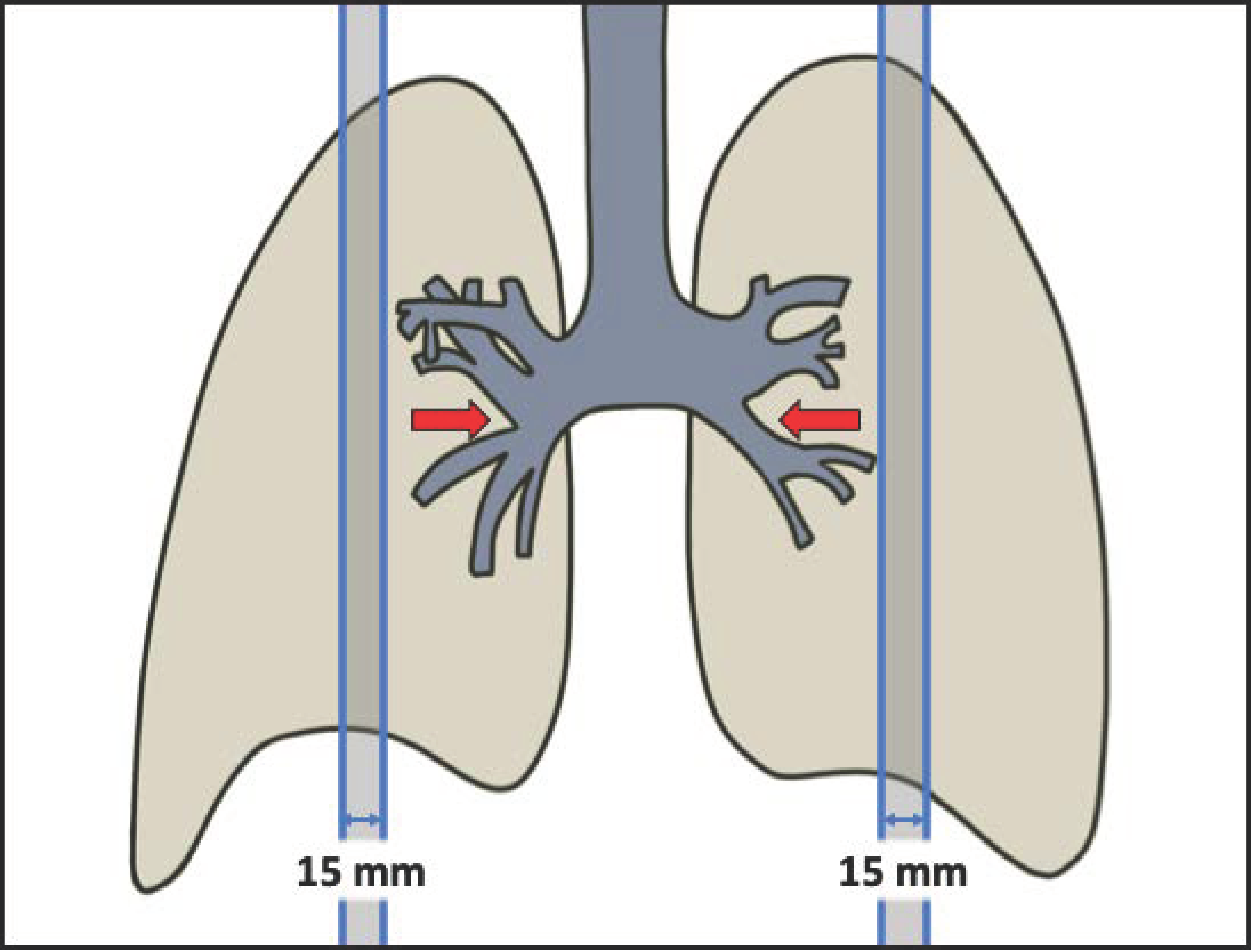
2.2. Image Acquisition

A fast gradient echo MR imaging sequence has been developed at the University of California, San Diego (UCSD) to spatially capture lung water density in CF subjects and healthy controls [26]. CF subjects with stable disease were recruited from the UCSD Adult CF clinic. Healthy adults without CF were recruited from the local population in San Diego. All subjects provided written informed consent approved by the Human Research Protections Program at UCSD (#110368).
MR density image data were acquired in an ACR accredited 1.5T GE EXCITE HDx Twinspeed MR imaging scanner (General Electric, Milwaukee, WI, USA) with imaging parameters kept within the established FDA guidelines for routine clinical MR examinations. Before being placed supine in the scanner, each subject was trained in breathing maneuvers to reach total lung capacity (TLC, full inspiration). The 3D maps of lung water density were collected with 15 mm thick sagittal slices (with no gap) encompassing the entire lung (15–18 2D sagittal slices) at TLC. Quantitative measurements of lung density were calculated as fractional lung density (FLD) with a range of values from 0 (100% air) to 1000 (100% fluid) on a voxel-by-voxel basis.
Quantitative measures of lung water density are based on data acquired with a multi-echo fast gradient echo (mGRE) sequence that acquires multiple single echo acquisitions within a single breath-hold. The sequence collects 12 images alternating between two echo times (TE = 1.0 and 1.8 ms) within a breath-hold. After averaging data at each echo time, data were fit on a voxel-by-voxel basis with a single exponential decay function to determine the local decay constant (T2*) and lung water content by back-extrapolating signal to an echo time of zero. Absolute water content was obtained with the inclusion of a phantom whose signal represents 100% water. Since the phantom does not have decay constants equal to that in the lung, a correction factor was empirically determined for the static sequence parameters (TR = 10 ms, T2 decay effects negligible), permitting the mean phantom signal to be used as a reference for absolute calibration of water content.

2.3. MR Tissue Density Data

The lung has been manually pre-processed and segmented from the surrounding structures in the 2D MR density images before the analysis is conducted in this study. We aim to quantify and analyze the spatial presentation of excess lung fluid (e.g., edema, peribronchial thickening, and bronchiectasis).
As MR density image data contains quantitative measurements of fractional lung density, large blood vessels are captured in the image and are difficult to distinguish from excess fluid when using thresholding techniques. We note that we do not currently have a method to remove the blood vessels in a repeatable and accurate manner. Therefore, a single 2D 15 mm sagittal slice lateral to the hilar vessels has been selected from the larger data set in each of the right and left lungs of each subject for analysis to avoid the added complexity of the blood vessels (Figure 1). Thus, a unique mask image that excludes all anatomy except lung tissue was generated for each of the 52 sagittal slice MR density images across the entire subject population. The advantage of utilizing image data devoid of blood vessels allows us to isolate and evaluate disease patterns for our early stage of model development before expanding our technique to the whole lung.
To address spatial variations in lung density, which must be accounted for when imaging supine at TLC, we have chosen to define regions of interest (ROIs) in a similar manner as in [27]. The masks were divided into nine ROIs by indexing their maximum anterior-posterior and cranial-caudal dimensions by thirds, effectively superimposing a 3 × 3 grid onto each mask. A 3 × 3 grid will sufficiently sample lung density within each ROI, ensuring the number of voxels within a grid is greater than 50 (the lowest adequate number of voxels to sufficiently sample lung density), along with the distribution of ROIs comprising the spatial variation of lung density observed.
The MR density image displays the lung density information (Figure 2), and the mask shows the total lung space encompassed by the sagittal slice while identifying the ROIs of the lung (Figure 2). In our analysis, the nine ROIs in the right lung are considered separately from the nine ROIs in the left lung (labeled regions 1–9 and regions 10–18, respectively) to account for physiological differences in right and left lung anatomy (Figure 2).

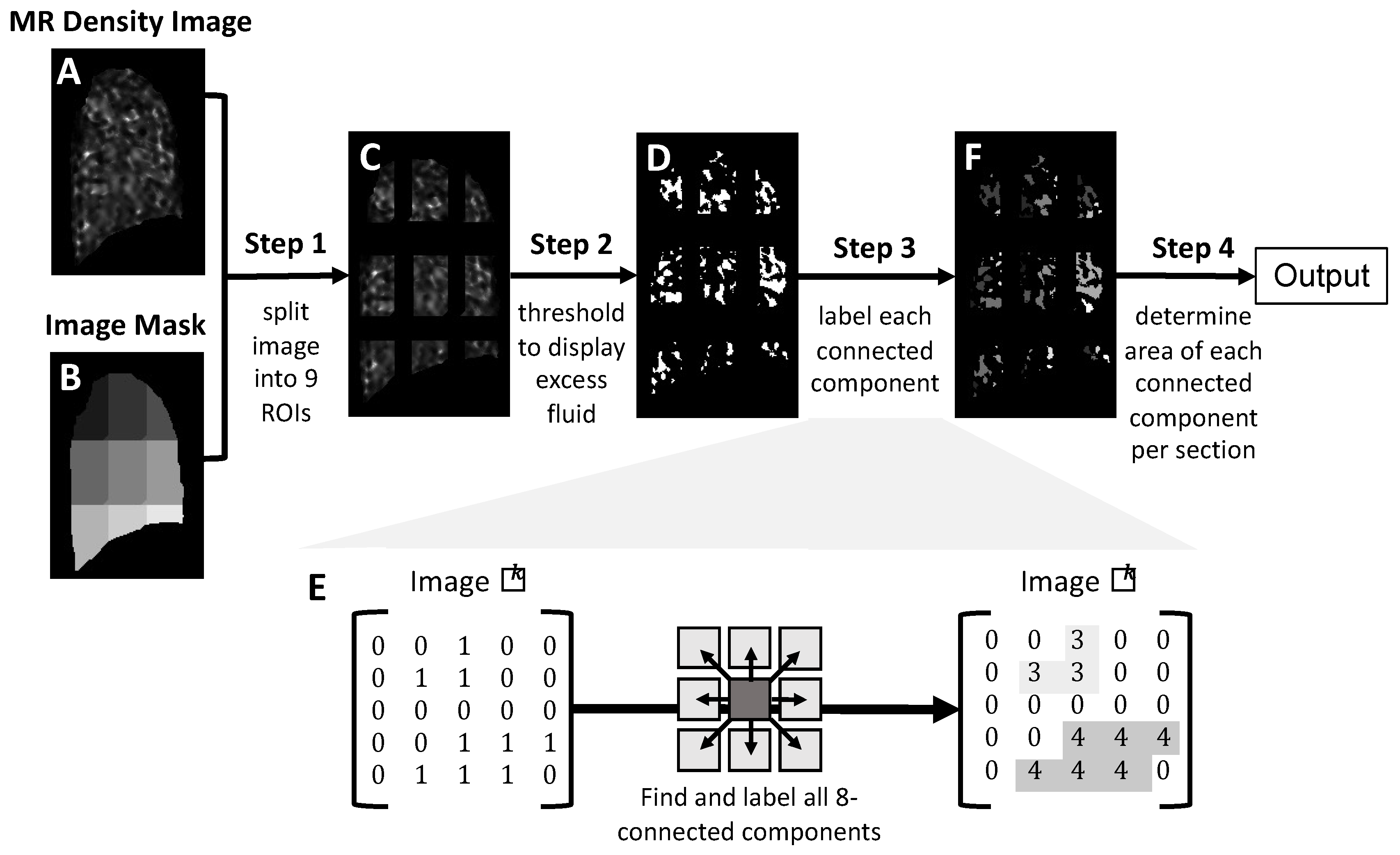
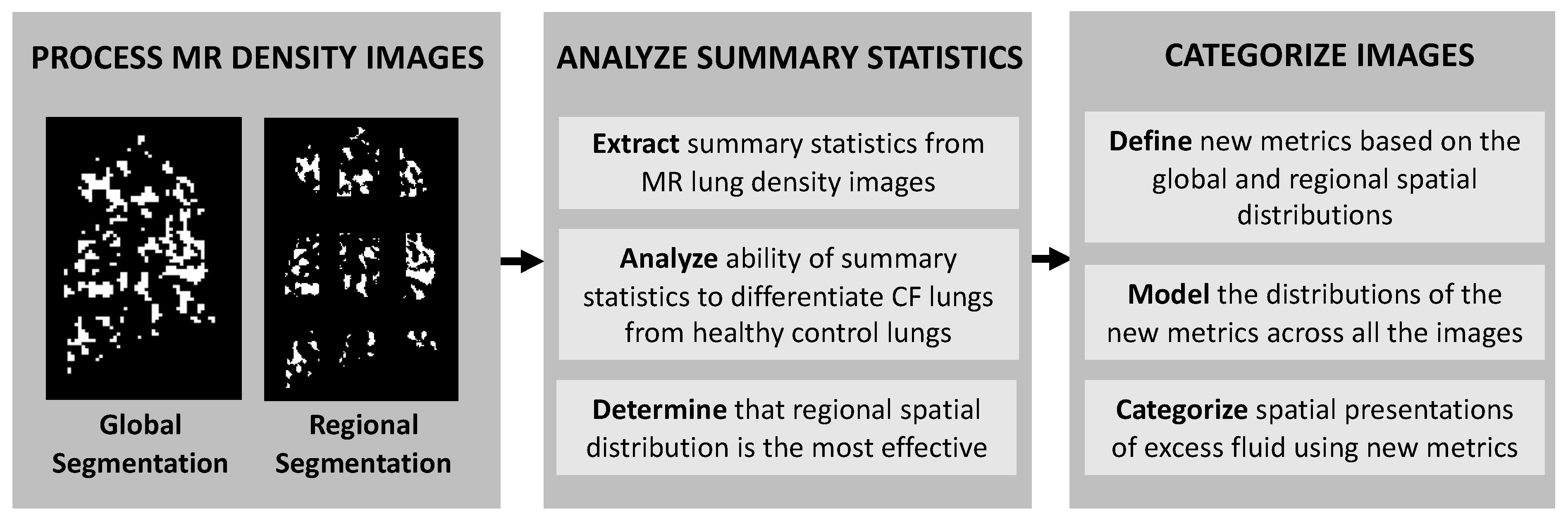
2.4. Image Processing and Analysis for Identification of Excess Lung Fluid in MR Lung Density Images

We have automated the extraction of excess fluid information from MR lung density images by writing a script that utilizes the MATLAB image processing toolbox. The data used for image processing has been described in Section 2.3. We begin with an MR lung density image and corresponding mask separated into nine ROIs.
When imported to MATLAB, each MR lung density image is represented by a matrix of pixel intensities. Following image import, the image processing technique follows four main steps: (i) the image is divided into the nine ROIs using an image mask, (ii) the excess lung fluid is segmented using a biologically relevant thresholding technique, (iii) connected components are identified, and (iv) the pixel areas of connected components are computed for each ROI. The data output includes a list of connected components, their areas, and the ROI in which each connected component was found. The image processing technique is described in detail throughout this section and summarized in Figure 3.

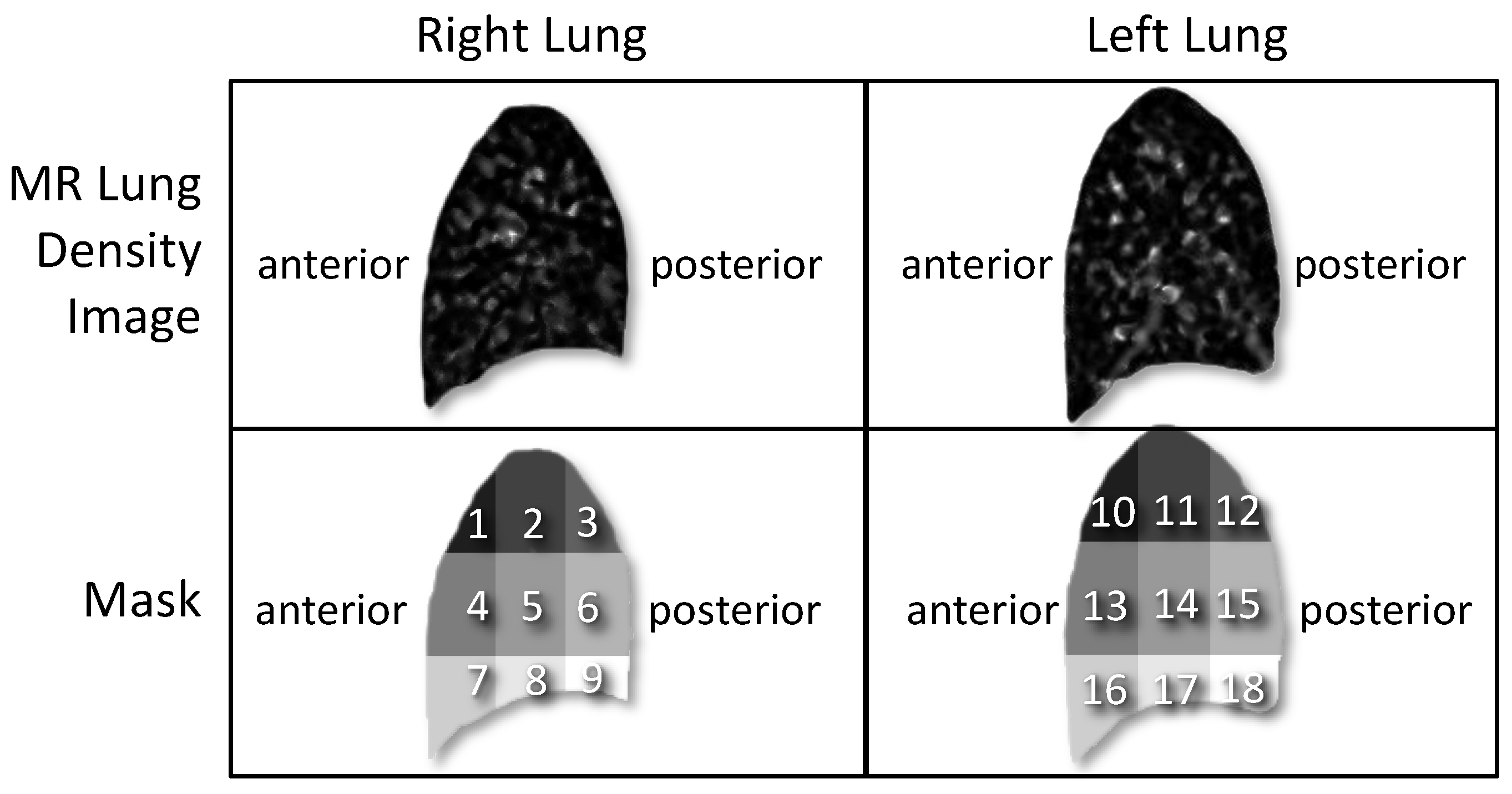
2.4.1. Division of MR Lung Density Image into Nine Regions of Interest (Step 1)

The inputs for the image processing technique are (i) an MR density image of a single sagittal slice of the lung (Figure 2 and Figure 3A) and (ii) an image mask that has been divided into nine ROIs by a 3 × 3 grid that is unique to each subject (Figure 2 and Figure 3B). The mask is used to divide the original image into nine ROIs by treating the one ROI as the foreground and removing the remainder of the image considered to be the background.

2.4.2. Images Are Thresholded to Identify Excess Lung Fluid (Step 2)

As described previously, MR density imaging captures the distribution of fluid in the lung by detecting the presence of water. In healthy lungs, water is detected in blood, lung tissue, and/or large blood vessels. In CF lungs, water is detected in not only healthy tissue but also in mucus and abnormal lung structures. Thus, images from healthy subjects comprise our control group, and the density of lung fluid in each ROI from this group is used to determine the presence of excess lung fluid. Each of the 18 ROIs are considered separately, as normal fluid and/or other anatomical structures do not occur uniformly across all ROIs [26]. The median of the pixel intensities within each ROI is computed using density images from the control group only. Intensities falling below two standard deviations of the control group’s median in each ROI represent normal lung fluid. These values become the threshold barriers for each ROI and are used to remove noise from the images by reassigning pixels below these barriers to an intensity value of 0. The remaining pixels represent excess lung fluid and are reassigned with an intensity value of 1. This step concludes with binarized images of each ROI displaying only excess fluid.

2.4.3. Identification of Connected Components (Step 3)

The third step in the image processing technique identifies connected components representing a collection of excess fluid. A collection of excess fluid may also be thought of as a cluster of excess fluid present in the image shown by white pixels, as in Figure 3D.
The image processing technique searches for an unlabeled pixel in the density image I and uses a flood-fill algorithm to label collections of pixels, which are groups of pixels that are 8-connected (i.e., their edges or corners touch) (Figure 3E). A flood-fill algorithm, sometimes called seed-fill, is a basic algorithm used in a variety of image processing applications and is described in its basic form in [28] and can be implemented using MATLAB version R2021b’s built-in functions bwconncomp and bwlabel. We label each connected component in the density image I uniquely using an integer and construct a new image L that contains the labeled connected components in the ROI. This step is repeated until all pixels have been labeled and the result is an image L that contains all the connected components and their respective labels (Figure 3F).

2.4.4. Quantification of Excess Fluid Collections (Step 4)

The image processing technique concludes by calculating the pixel area of each connected component and recording the location (ROI) in which it was found. The area of each labeled connected component is defined as the total number of pixels within that label. At this stage, we can easily identify each collection of excess fluid and its respective pixel area in each ROI by the unique labels generated in step 3. The output is the pixel area of each labeled connected component per ROI.

2.5. Statistical Analysis

We aim to identify the key statistics that distinguish the presence of excess fluid in CF subjects from healthy controls by evaluating features for statistical significance. The statistical significance of the differences between the CF and control groups was determined by a two-sample non-parametric Kruskal–Wallis test. Distribution fits were assessed for statistical significance using a one-sample Kruskal–Wallis test on the transformed data. A non-parametric test was chosen due to the smaller sample size and to avoid unnecessary distribution assumptions. Statistical significance was taken at the 95% confidence level. Statistical tests were performed using R (RStudio version 1.4.1106).

3. Results

Using the methods described, MR density images have been processed to identify collections of excess fluid in the lungs. We aim to describe the collections by first determining the key summary statistics capturing differences in CF vs. control, identifying these differences across both global and regional lung space, and finally labeling the spatial presentation of excess fluid in the lungs. An overview of the workflow is shown in Figure 4.

3.1. Summary Statistics of Excess Fluid in MR Lung Density Image: CF vs. Control

We have implemented the image processing technique for lung MR density images from healthy controls (CTL, n = 13) and CF subjects with mild (n = 4), moderate (n = 5), and severe (n = 4) disease. Images of the right and left lungs were considered separately for a total of 52 individual MR images, 26 in the left and 26 in the right.
From the data output, we have determined summary statistics in each of the nine ROIs per lung for both healthy controls and CF subjects. Summary statistics include mean connected component area, maximum connected component area, the number of connected components, and the area of excess fluid, with respect to lung size, which we define as spatial distribution.

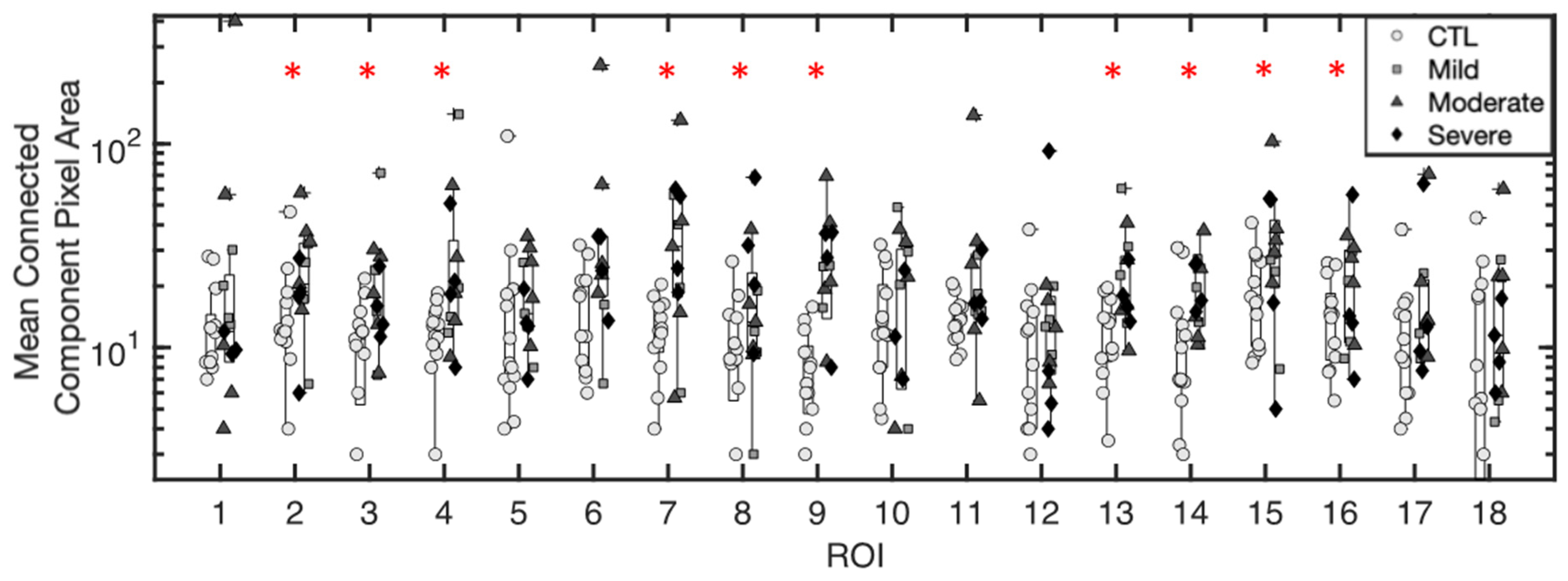
3.1.1. Mean Pixel Area of Excess Fluid Collections

The mean connected component area in each of the 18 ROIs (9 in the right lung, 9 in the right) has been evaluated to investigate if CF subjects have larger collections of excess fluid, compared to healthy control subjects. The median was not chosen for investigation because we aim to extract the extreme behaviors occurring within the CF population. Figure 5 shows the mean connected component pixel area across all 18 lung ROIs in the right and left lungs for individuals with different CF severity levels and healthy controls. We found a statistically significant increase in the mean connected component area for CF subjects from that of healthy controls in 10 out of the 18 regions (p < 0.05, red asterisks in Figure 5).

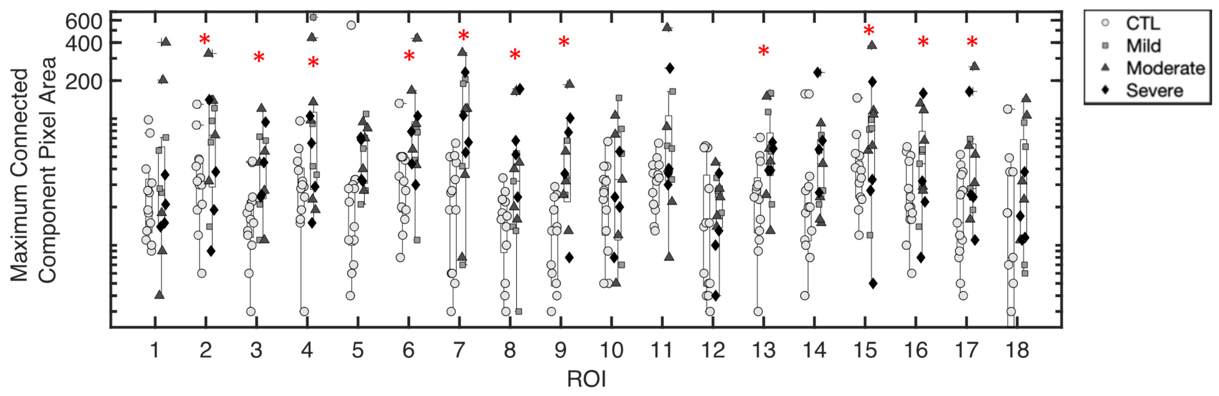
3.1.2. Maximum Pixel Area of Excess Fluid Collections

The maximum connected component area was evaluated for all CF and healthy control subjects in each ROI (Figure 6). The maximum connected component area was found to be statistically greater for CF subjects, when compared to healthy controls in 11 out of the 18 regions (p < 0.05, red asterisks in Figure 6).

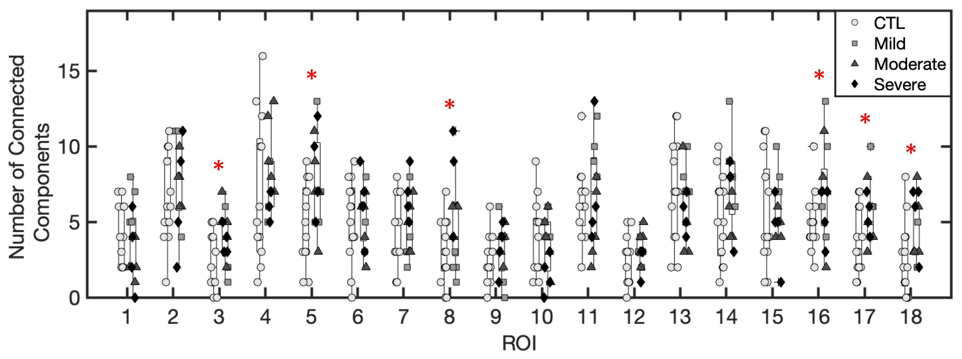
3.1.3. Number of Excess Fluid Collections

The number of connected components per ROI is shown in Figure 7. Compared to the mean and maximum connected component area (Figure 5 and Figure 6), the number of connected components did not show many extremes in the form of outliers in CF subjects. There was a statistically significant increase in the number of connected components for CF subjects when compared to healthy controls in 6 out of the 18 regions (p < 0.05, red asterisks in Figure 7). The number of connected components per ROI did not distinguish CF from control subjects in most ROIs. This is not surprising because this metric does not account for the connected component area. A CF subject may have the same number of connected components as a healthy control subject, but those of the CF subject may be larger.

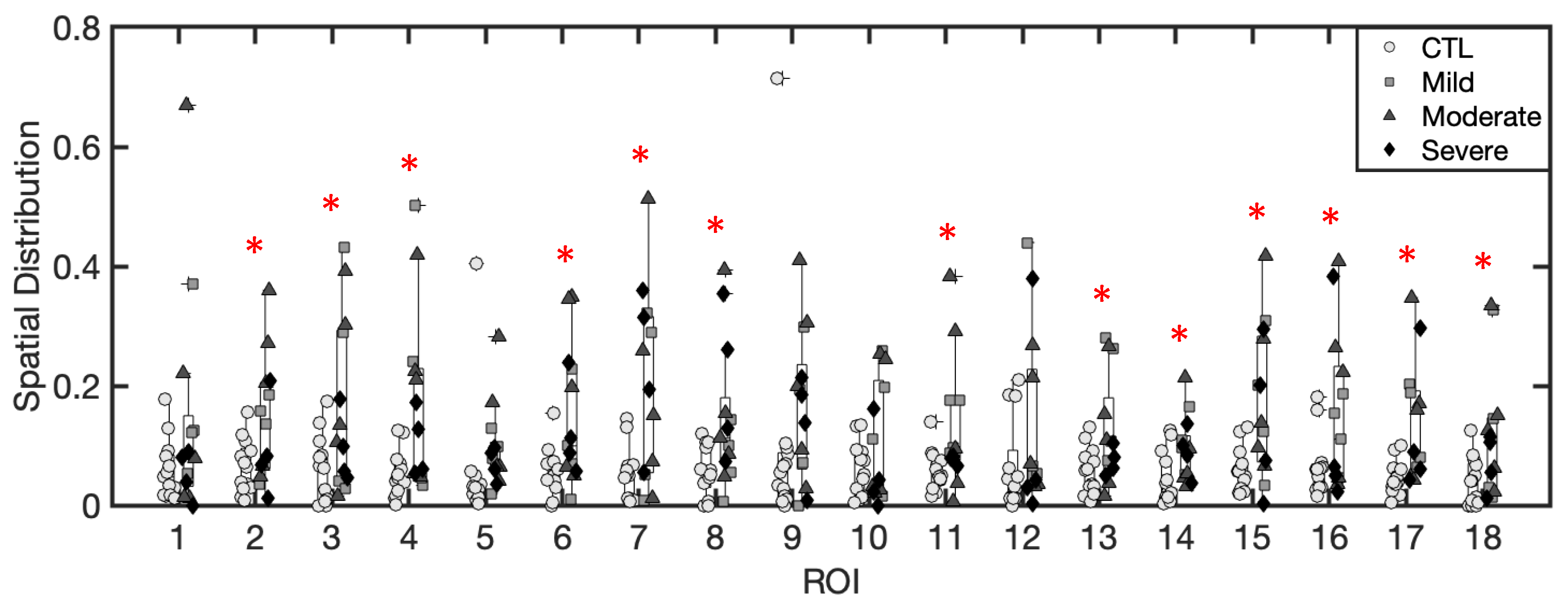
3.1.4. Spatial Distribution of Excess Fluid Collections

Spatial distribution is defined as the percentage of excess fluid in an ROI. Here, we define this as S D R O I which gives the percent of the ROI that is covered by excess fluid (Definition 1).
Definition 1.
The spatial distribution of a region of interest of the lung is defined as the area of excess lung fluid in the region of interest ( A R O I F ) divided by the area of the region of interest  ( A R O I ) .   That is:
S D R O I = A R O I F A R O I   .
We found that   S D R O I distinguished CF from healthy control subjects overwhelmingly. Figure 8 shows the spatial distribution of fluid values for all ROIs in both the right and left lungs across all groups. There was a statistically significant increase in spatial distribution for CF subjects when compared to controls in 13 out of the 18 regions (p < 0.05, red asterisks in Figure 8).

3.1.5. Inference of Summary Statistic Importance

After an analysis of the mean connected component area, the maximum connected component area, the number of connected components and the spatial distribution of excess fluid in each ROI for both CF subjects and healthy controls, we conclude that spatial distribution distinguishes CF lungs from healthy control lungs in the most comprehensive manner. We note that since lung size varies across subjects, the spatial distribution allows for the comparison of the proportion of the lung covered by excess mucus across subjects. Therefore, spatial distribution incorporates not only the amount (area) of excess lung fluid in an ROI but also the lung space occupied by the ROI, as this is not uniform across subjects. In the following, we group the spatial presentation of excess fluid in CF and control lungs by using information from the spatial distribution of abnormal fluid.

3.2. Regional and Global Spatial Distribution of Excess Lung Fluid

We have identified S D R O I as the parameter that distinguishes CF subjects from healthy controls. We note that S D R O I measures the regional distribution of excess lung fluid. To assess the proportion of a whole lung covered by excess fluid, we introduce S D W as the proportion of the whole lung covered by excess fluid. A higher S D W represents a lung that has a high percentage of excess fluid coverage overall.
We define a focality of excess lung fluid as a concentration of fluid in a particular lung ROI. We use diffuse to refer to excess fluid that is evenly distributed throughout lung ROIs. To quantify the distribution of focal and diffuse fluid, the S D W and a spread of S D R O I (see Definition 2) values in each lung were used.
Definition 2
If the set SD contains all  S D R O I values for a lung, i.e.,  S D = { S D 1 ,   S D 2 , ,   S D 9 } , then the spread of  S D R O I values is given by
R = max S D min S D .
A low R means the S D R O I values across the lung are showing low variability, or diffuse spatial presentation. A high R means the S D R O I values across the lung may be higher in one area than another, signifying one or more focalities of excess fluid are present.
We identified normal, moderate, and extreme values of R and S D W by implementing a distribution analysis. The right and left lung were analyzed separately and the distribution of the R values across all samples (CF and control) was found to be lognormal (p < 0.01). Similarly, the S D W metric was found to have a lognormal distribution (p < 0.01).
In Figure 9, the lognormal distribution curves for S D W and R metrics are divided into three sections based on the mean ( μ ) and the standard deviation ( σ ) for the distribution. Critical values for the R metric given in Table 1 are identified by the mean μ R and standard deviation   σ R : 0.18 and 0.35, which are μ R and μ R + σ R , respectively. Similarly, for the S D W metric with mean μ SD W and standard deviation σ SD W , the critical values are 0.1 and 0.19 for μ SD W and μ SD W + σ SD W , respectively. These critical values identify the ranges a S D W value or R value must fall within to be identified as one of the three categories for an S D W value (i.e., S1, S2, S3) and the three categories for an R value (i.e., R1, R2, R3) (Table 1, Figure 8).

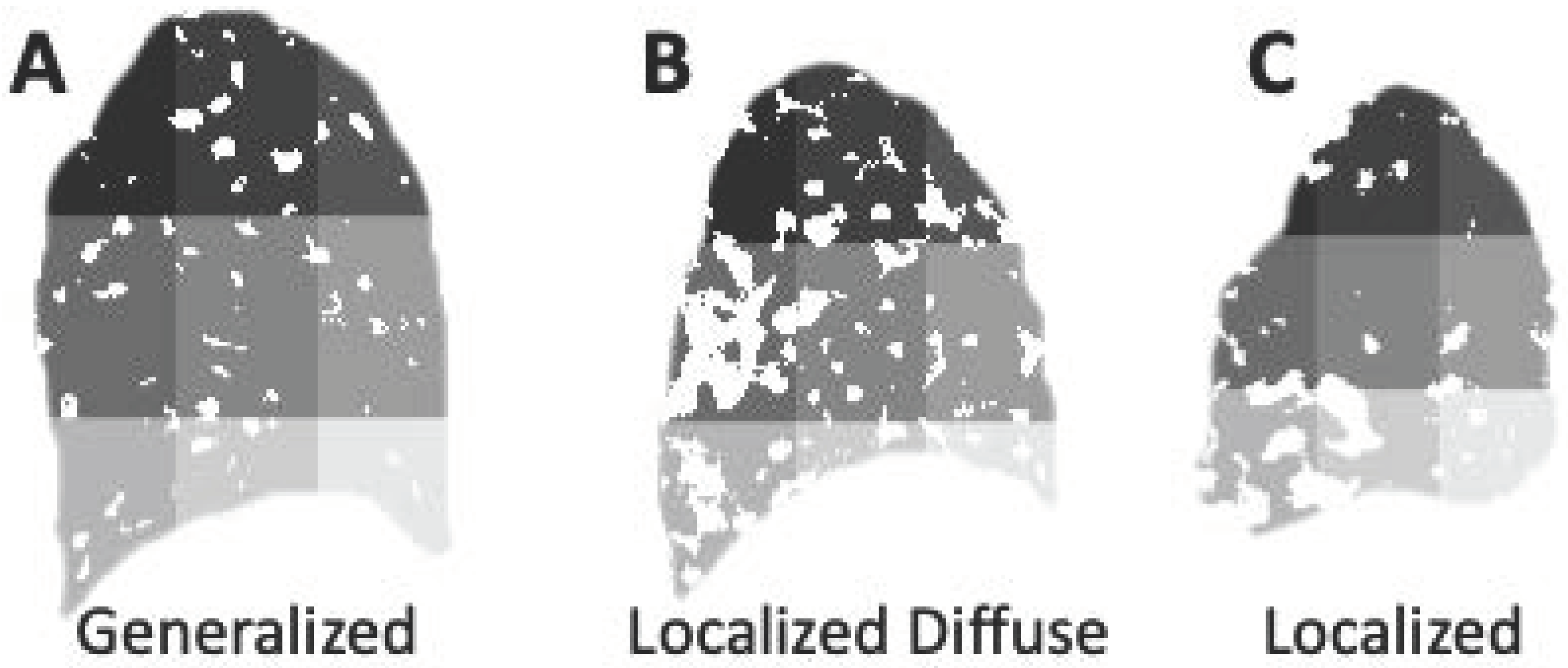
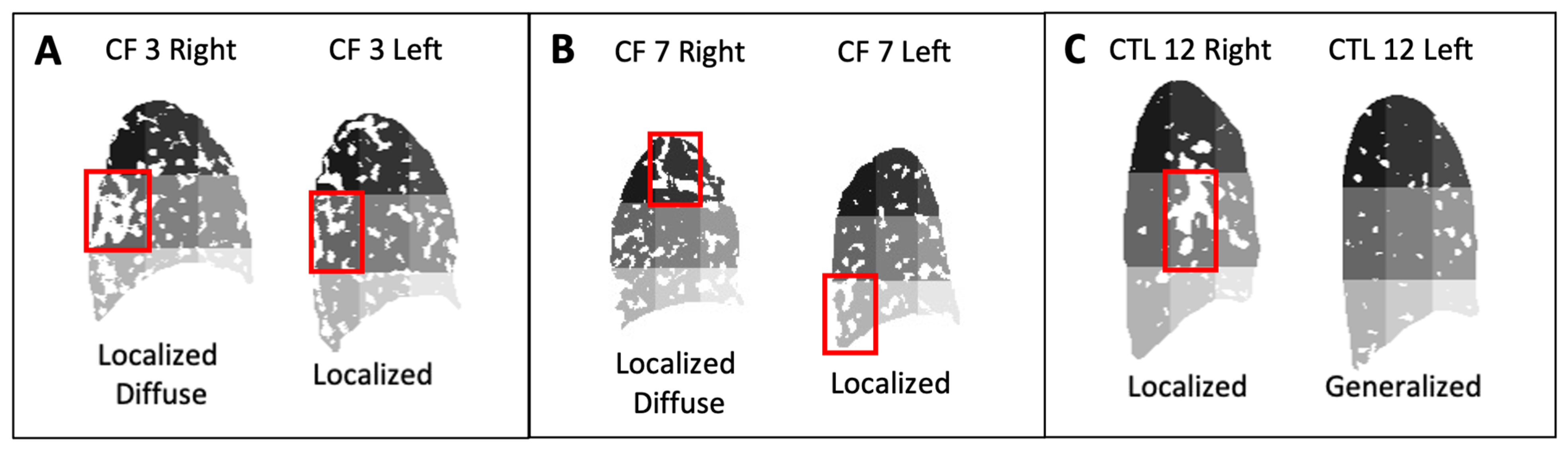
3.3. Categories of the Spatial Presentation of Excess Lung Fluid: Generalized, Localized Diffuse and Localized Presentations

S D W yields information about the percent of the lung that is covered by excess lung fluid while R identifies the range of excess lung fluid across the nine lung ROIs. Each 2D lung density image has been assigned an S D W category (S1, S2, or S3) and an R category (R1, R2, or R3). We assign the spatial presentation of a lung’s excess fluid into one of three distinct categories by using a combination of the S D W and R metrics. These spatial presentations are (i) generalized presentation, (ii) localized diffuse presentation, and (iii) localized presentation. (Table 2). Sample lung images for these spatial presentations are shown in Figure 10.

3.3.1. Generalized Spatial Presentation of Excess Lung Fluid

Generalized spatial presentation is defined by excess fluid that occurs uniformly throughout the lung. With respect to our metrics, a generalized spatial presentation has a low S D W value (category S 1 or S 2). A lung in the S 1 category has a low percent coverage of excess lung fluid, and the collections identified are often small in pixel area and sparse throughout the lung.
For a lung in the R1 category, regardless of the S D W value, the presence of excess lung fluid in the lung is approximately uniform across the nine ROIs. Therefore, any lung with an R1 category is also considered to have a generalized spatial presentation (Table 2). As can be seen in Figure 10A, a generalized spatial presentation has a low overall amount of excess lung fluid spread evenly throughout the nine ROIs.

3.3.2. Localized Diffuse Spatial Presentation of Excess Lung Fluid

Localized diffuse spatial presentation is defined by excess fluid that occurs with a strong focality in an ROI, with a high overall density of excess fluid present within that ROI. Figure 10B demonstrates a localized diffuse spatial presentation where there is a concentration of excess fluid in ROI 4 with a high percentage of excess fluid in the remaining ROIs. A localized diffuse spatial presentation has a severe S D W value (category S3) and a moderate or severe R value (category R2 or R3).
A lung in the S3 category has a large amount of excess lung fluid in the lung. The R2 and R3 categories demonstrate that even with a large amount of excess lung fluid, there is a concentration of this fluid in a particular ROI or ROIs (Table 2).

3.3.3. Localized Spatial Presentation of Excess Lung Fluid

A localized spatial presentation is used to describe excess fluid that has a clear and strong localization in a particular ROI. A localized spatial presentation has a moderate S D W value, but the R value is moderate to severe due to a large concentration of excess lung fluid. Therefore, localized spatial presentation is used to characterize a lung in the S2 category that is also in an R2 or R3 category (Table 2). Figure 10C shows a localized spatial presentation where there is a collection of excess fluid in ROI 7.

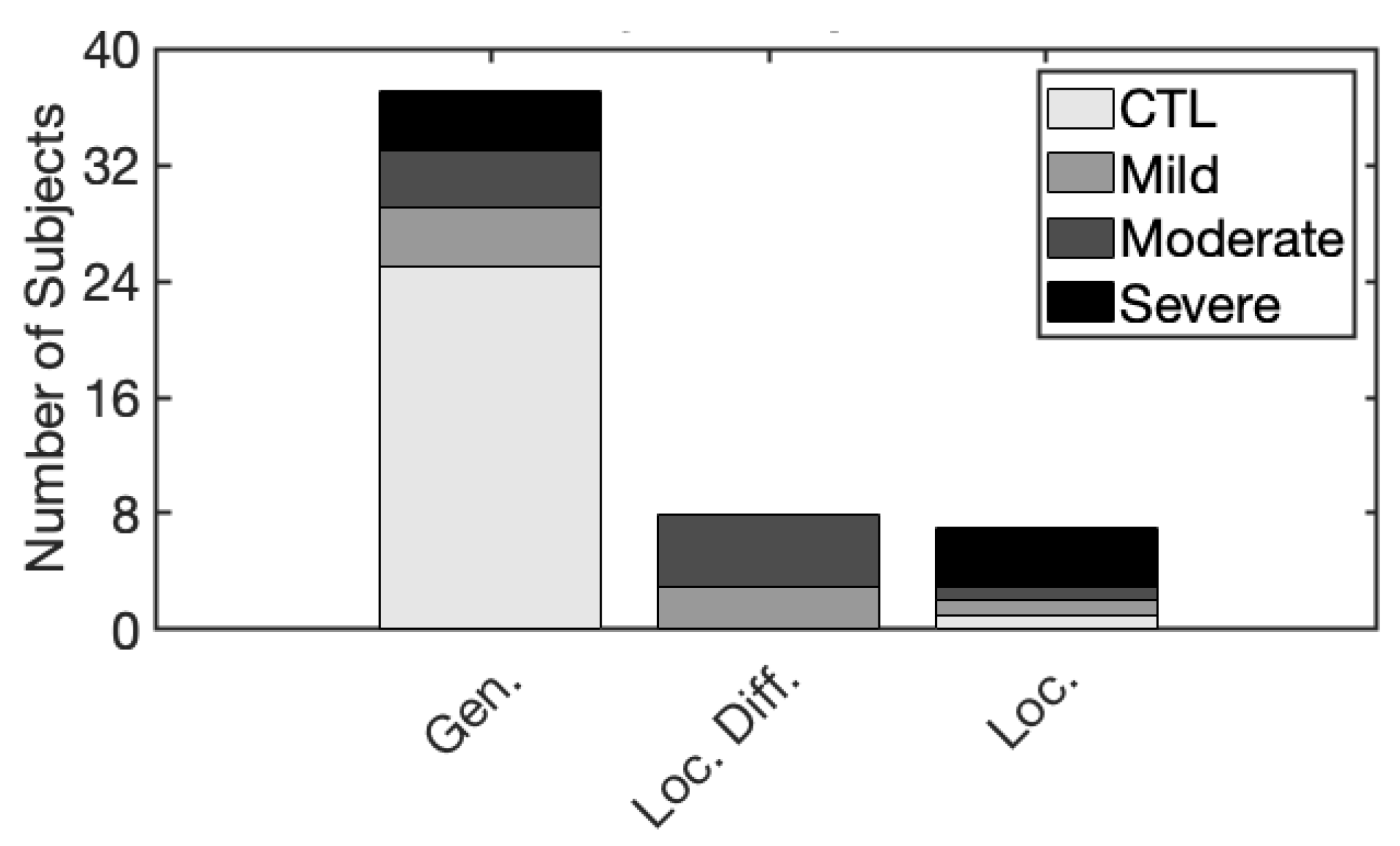
3.3.4. Summary of Spatial Presentation Groups

A summary of spatial presentation assignments is presented in Table 3 for healthy controls and CF subjects with mild, moderate, and severe disease. As expected, our model assigns most control lungs to the generalized spatial presentation, with only one control lung not generalized but localized with a statistically significant difference in spatial presentation among CF and CTL (Figure 11, p < 0.01 Fisher’s exact test). CF lungs are found in all three spatial presentation groups. It is important to note that the 13 CF subjects have varying severity levels. Six of the thirteen CF subjects were assigned the generalized spatial presentation in both the right and left lung: two mild, two moderate, and two severe CF subjects (Table 3). Three CF subjects (two moderate and one mild CF subject) were assigned a localized diffuse spatial presentation in both the right and left lung (Table 3). Two subjects with severe CF were assigned the localized spatial presentation in both the right and left lung (Table 3). Only two CF subjects (one mild and one moderate CF subject) had different spatial presentation assignments for their right and left lung. Their right lungs were assigned a localized spatial presentation, while their left lungs were assigned a localized diffuse spatial presentation (Table 3).

4. Discussion

In this study, we aimed to quantitatively describe the spatial presentation of excess fluid in CF. MR lung density images that identify excess fluid indicative of lung abnormalities were obtained for 13 CF subjects across mild-to-severe disease severity and age- and sex-matched healthy control subjects. We implemented a thresholding-based image processing technique that segments excess fluid in the lungs using healthy controls as a baseline and developed novel metrics to quantify the spatial presentations of the excess lung fluid. We characterized the spatial presentations of excess fluid in each CF subject and healthy control subject based on the location, size, and density of excess fluid present in different regions of their lungs. The percent area of excess fluid, referred to as the spatial distribution, was computed for the total lung and different regions of interest. We found that the spatial distribution was a key factor in identifying the differences in spatial presentation between CF and control subjects. We developed metrics based on spatial distribution to capture differences in excess fluid regionally and globally. These metrics were used to define the spatial presentation of each lung in one of three groups: (i) generalized if the fluid was sparse, (ii) localized diffuse if at least one focality of fluid was present with a dense distribution of fluid elsewhere, and (iii) localized if at least one focality of fluid was present with a sparse distribution. With our metrics, we found that 96% of our healthy control subjects exhibited a generalized spatial pattern. Conversely, CF subjects made up 93% of the localized and localized diffuse spatial patterns (Figure 11). A key contribution from this study is the ability to characterize CF subjects into groupings based on the anatomical features of their disease using an automated methodology, eliminating the potential for variability due to manual annotation. This study is the first of its kind, to our knowledge, to identify and characterize the spatial presentation of CF disease in this way.
An interesting finding is the spatial presentation of a subject was not always identical in both lungs. Two CF subjects had varying spatial presentations in either lung, CF 3 and CF 7, along with one control subject (Table 3, Figure 12A,B). This response suggests the heterogeneity of lung fluid density even within one subject. The amount of excess fluid present in the lung plays a large role in the spatial presentation ultimately used to categorize the subject. As an example, we can see that in Figure 12B, CF 7 has a strong localization of fluid in the bottom anterior ROI 16 with a large amount of fluid elsewhere. The spread of the excess fluid is otherwise low, as the percent coverage across all ROIs are similar. CF 3 also had differing spatial presentations in the right and left lung (Figure 12A). In this case, the left lung is on the outer boundary of a localized distribution where a small increase in total coverage ( S D W ) would lead to a localized diffuse category (Table 3). The metrics defined in this study can identify these subtle characteristics that distinguish one lung from the next with sensitivity to category boundaries.
Additionally, we grouped the spatial presentation of a control subject (CTL 12) as generalized in the left lung and localized in the right (Figure 12C). In this particular case, we hypothesize the localization was due to the hilar vessels being present in the image. As seen in Figure 12C, the localization of excess lung fluid is in the center of the lung where large blood vessels are present. To the best of our ability, we aimed to choose a slice of the lung that was lateral to the hilar vessels while maintaining equidistance between the left and right lung images chosen. Subjects with narrow lungs have fewer 15 mm slices making up their total lung volume, therefore, limiting our ability to exclude the hilar vessels. The discussion of this control sample is essential, as this is the only control subject not in the generalized spatial presentation group. It is important to note that the remaining anatomy shows sparse excess fluid, which is expected for healthy control subjects.
The image processing technique and metrics developed focus on segmenting and identifying excess lung fluid through comparison to healthy control subjects. This comparative approach for identifying excess fluid may be used to analyze images using other quantitative imaging techniques. For instance, CT images will differ from MR images because CT tissue density includes non-water components from lung tissue, but both imaging techniques measure the presence of fluid in the lungs. Thus, our methodology may be applied to investigate whether differences between CF and healthy control subjects can be observed in a variety of other imaging studies.
Unlike many other genetic diseases, CF patients have access to therapies developed to target specific CFTR gene mutations [29]. Though not a cure, four separate FDA-approved CFTR modulator therapies have brought hope to CF patients and their families by treating the defect directly instead of treating symptoms [30,31]. In late October 2019, the most recent CFTR modulator therapy was FDA approved. The triple combination of elexacaftor/tezacaftor/ivacaftor (TrikaftaTM, Vertex Pharmaceuticals Inc., Boston, MA, USA) has been designed to treat CF patients with one copy of the F508del mutation benefiting 90% of the CF patient population [32,33]. With FEV1 being the primary efficacy endpoint in CFTR modulator clinical trials, there is limited information on how, and to what degree, these therapies have on regional lung structure [34,35,36].
While imaging studies have not been used in CFTR modulator clinical trials, there are a few observational imaging studies in patients treated with CFTR therapy. Consequently, there is limited information on the nature of how CFTR therapy alters the underlying structural implications of CF. To date, there are four computed tomography studies (CT) [37,38,39,40]. These studies have reported decreases in peribronchial thickening and mucus plugging along with ventilatory improvements utilizing the Brody CT scoring system [5] in response to CFTR modulator therapy. None of these studies have developed a metric or utilized metrics which present the degree and severity of heterogeneity observed across the CF population. Through the implementation of our metrics, we can determine the scope of what remains after CFTR therapy, such as whether a specific type of heterogeneity (localized vs. diffuse disease) progresses at a different rate. In conjunction with clinical classification (FEV1), our spatial presentation groupings have the potential to be employed to guide these therapies and assess changes in disease status and response to treatment.
In recent years, image analysis algorithms have significantly aided the study of lung diseases [41,42,43,44]. The majority of image analysis algorithms for studying lung disease focus on tissue segmentation [45,46,47,48,49]. The field has been enhanced by innovations in the field of machine learning, such as the development of the convolutional neural network (CNN), a machine learning tool that uses imaging data to accomplish predictive tasks without the need for human interference. A study by Marques et al. [50] used CNNs to detect the presence of structural abnormalities in lung tissues and classified CF CT images as bronchiectasis, atelectasis, or mucus plugging. Although promising, the CNNs developed and utilized to date for lung analysis have significant limitations. CNNs are typically trained through supervised methods, meaning both their inputs (e.g., medical images) and their labels (e.g., clinical outcomes) are used to train a model. Additionally, for a well-behaved model, a large number of previously annotated outcomes are necessary for training. Many studies have been published that attempt to limit the need for a large number of training data for neural networks, but there are currently no effective methods and algorithms for it [51].
To our knowledge, the spatial presentation of excess lung fluid in the lung has yet to be defined and characterized. This study has developed a methodology to define spatial presentation outcomes for CF subjects. Additionally, the automated process eliminates the need for clinical outcomes to be defined manually and reduces the possibility of human subjectivity upon characterization. The methodology and results of this study may be used to develop a larger database of spatial presentation outcomes for further headway towards complete automation of medical image analysis for this problem using CNNs.
The results of this study should be interpreted with some limitations in mind. This study made use of one 15 mm sagittal slice (i.e., a 2D image) representing lung density within the 15 mm volume in the right lung and left lung lateral to the hilar vessels for analysis. We have intentionally chosen this route to build a technique to characterize the spatial presentation of excess lung fluid while avoiding the added complexities within the lung that may skew data, such as the consideration of large blood vessels, a normal feature in lung anatomy. Although this may be a limitation currently, the methodology developed in this study may be used as a first step toward an analysis incorporating the entire lung. A possible extension would be the evaluation of all 2D sagittal slices that complete the volumetric MR map of lung density. Each 2D slice may be analyzed independently utilizing the same methodologies with only mild modifications. Because the spatial consequences of CF do not occur uniformly throughout the lung, a 3D analysis of the lungs will likely yield additional information about the disease.
In this study, we have developed a methodology to quantify the spatial heterogeneity of CF disease in 2D images of the lungs. The results of this study suggest that the spatial characteristics of CF may be used in conjunction with existing measurements, such as FEV1, to investigate the link between lung function and disease status. Our methods motivate the need for more comprehensive studies as to how the distribution of lung abnormalities affects disease progression, response to medicinal drugs, and overall lung health [5,6,52]. The extensions of this work through future studies with larger sample sizes may increase the possibility for personalized diagnoses and treatment plans.

Author Contributions

Conceptualization, A.V.S., A.N.L., R.J.T. and U.Z.G.; methodology, A.V.S., A.N.L., R.J.T. and U.Z.G.; software, A.V.S. and A.N.L.; validation, A.V.S., A.N.L., R.J.T. and U.Z.G.; formal analysis, A.V.S., A.N.L., R.J.T. and U.Z.G.; image acquisition, R.J.T.; writing—original draft preparation, A.V.S., A.N.L., R.J.T. and U.Z.G.; writing—review and editing, A.V.S., A.N.L., R.J.T. and U.Z.G.; visualization, A.V.S., A.N.L., R.J.T. and U.Z.G.; supervision, R.J.T. and U.Z.G.; funding acquisition, A.V.S., A.N.L., R.J.T. and U.Z.G. All authors have read and agreed to the published version of the manuscript.

Funding

U.Z.G. acknowledges support from the California State University Program for Education & Research in Biotechnology New Investigator grant. A.V.S. and U.Z.G. acknowledge support from the College of Sciences at San Diego State University. A.V.S. was supported by the ACM SIGHPC Computational & Data Science Fellowship. A.N.L. was supported by the NIH IMSD Program Grant 5R25GM058906. A.V.S. and A.N.L. acknowledge support from NSF STEM Scholar Award #1930546. R.J.T. acknowledges support from NIH grants R21 EB015579 and R01 HL135496.

Institutional Review Board Statement

The study was conducted in accordance with the Declaration of Helsinki, and approved by the Institutional Review Board of the University of California, San Diego (protocol code 110368, date of approval 3/3/2011).

Informed Consent Statement

Informed consent was obtained from all subjects involved in the study.

Data Availability Statement

The MR imaging data used in this study is not publicly available due to ethical concerns.

Conflicts of Interest

The authors declare no conflict of interest.

References

  1. Ramsey, B.W.; Downey, G.P.; Goss, C.H. Update in Cystic Fibrosis 2018. Am. J. Respir. Crit. Care Med. 2019, 199, 1188–1194. [Google Scholar] [CrossRef] [PubMed]
  2. Quinton, P.M. Role of epithelial HCO3 transport in mucin secretion: Lessons from cystic fibrosis. Am. J. Physiol. Cell Physiol. 2010, 299, C1222–C1233. [Google Scholar] [CrossRef] [PubMed] [Green Version]
  3. Chmiel, J.F.; Davis, P.B. State of the art: Why do the lungs of patients with cystic fibrosis become infected and why can’t they clear the infection? Respir. Res. 2003, 4, 8. [Google Scholar] [CrossRef] [PubMed] [Green Version]
  4. Horsley, A.; Siddiqui, S. Putting lung function and physiology into perspective: Cystic fibrosis in adults. Respirology 2015, 20, 33–45. [Google Scholar] [CrossRef]
  5. Brody, A.S.; Kosorok, M.R.; Li, Z.; Broderick, L.S.; Foster, J.L.; Laxova, A.; Bandla, H.; Farrell, P.M. Reproducibility of a scoring system for computed tomography scanning in cystic fibrosis. J. Thorac. Imaging 2006, 21, 14–21. [Google Scholar] [CrossRef]
  6. Cutting, G.R. Cystic fibrosis genetics: From molecular understanding to clinical application. Nat. Rev. Genet. 2015, 16, 45–56. [Google Scholar] [CrossRef] [Green Version]
  7. Collaco, J.M.; Blackman, S.M.; McGready, J.; Naughton, K.M.; Cutting, G.R. Quantification of the relative contribution of environmental and genetic factors to variation in cystic fibrosis lung function. J. Pediatr. 2010, 157, 802–807.e73. [Google Scholar] [CrossRef] [Green Version]
  8. Verschakelen, J.A.; Van fraeyenhoven, L.; Laureys, G.; Demedts, M.; Baert, A.L. Differences in CT density between dependent and nondependent portions of the lung: Influence of lung volume. AJR Am. J. Roentgenol. 1993, 161, 713–717. [Google Scholar] [CrossRef]
  9. Mumcuoglu, E.U.; Long, F.R.; Castile, R.G.; Gurcan, M.N. Image analysis for cystic fibrosis: Computer-assisted airway wall and vessel measurements from low-dose, limited scan lung CT images. J. Digit. Imaging 2013, 26, 82–96. [Google Scholar] [CrossRef] [Green Version]
  10. Bonnel, A.S.; Song, S.M.-H.; Kesavarju, K.; Newaskar, M.; Paxton, C.J.; Bloch, D.A.; Moss, R.B.; Robinson, T.E. Quantitative air-trapping analysis in children with mild cystic fibrosis lung disease. Pediatr. Pulmonol. 2004, 38, 396–405. [Google Scholar] [CrossRef]
  11. Brasfield, D.; Hicks, G.; Soong, S.; Tiller, R.E. The chest roentgenogram in cystic fibrosis: A new scoring system. Pediatrics 1979, 63, 24–29. [Google Scholar] [CrossRef]
  12. de Jong, P.A.; Mayo, J.R.; Golmohammadi, K.; Nakano, Y.; Lequin, M.H.; Tiddens, H.A.; Aldrich, J.; Coxson, H.O.; Sin, D.D. Estimation of cancer mortality associated with repetitive computed tomography scanning. Am. J. Respir. Crit. Care Med. 2006, 173, 199–203. [Google Scholar] [CrossRef]
  13. Huda, W. Radiation doses and risks in chest computed tomography examinations. Proc. Am. Thorac. Soc. 2007, 4, 316–320. [Google Scholar] [CrossRef]
  14. Fuchs, S.I.; Gappa, M.; Eder, J.; Unsinn, K.M.; Steinkamp, G.; Ellemunter, H. Tracking Lung Clearance Index and chest CT in mild cystic fibrosis lung disease over a period of three years. Respir. Med. 2014, 108, 865–874. [Google Scholar] [CrossRef] [PubMed] [Green Version]
  15. Loeve, M.; Lequin, M.H.; de Bruijne, M.; Hartmann, I.J.; Gerbrands, K.; van Straten, M.; Hop, W.C.; Tiddens, H.A. Cystic fibrosis: Are volumetric ultra-low-dose expiratory CT scans sufficient for monitoring related lung disease? Radiology 2009, 253, 223–229. [Google Scholar] [CrossRef]
  16. O’Connor, O.J.; Vandeleur, M.; McGarrigle, A.M.; Moore, N.; McWilliams, S.R.; McSweeney, S.E.; O’Neill, M.; Chroinin, M.N.; Maher, M.M. Development of low-dose protocols for thin-section CT assessment of cystic fibrosis in pediatric patients. Radiology 2010, 257, 820–829. [Google Scholar] [CrossRef] [Green Version]
  17. Altes, T.A.; Eichinger, M.; Puderbach, M. Magnetic resonance imaging of the lung in cystic fibrosis. Proc. Am. Thorac. Soc. 2007, 4, 321–327. [Google Scholar] [CrossRef]
  18. Eichinger, M.; Eichinger, M.; Puderbach, M. Computed Tomography and Magnetic Resonance Imaging in Cystic Fibrosis Lung Disease. J. Magn. Reson. Imaging 2010, 32, 1370–1378. [Google Scholar] [CrossRef]
  19. Eichinger, M.; Optazaite, D.E.; Kopp-Schneider, A.; Hintze, C.; Biederer, J.; Niemann, A.; Mall, M.A.; Wielpütz, M.O.; Kauczor, H.U.; Puderbach, M. Morphologic and functional scoring of cystic fibrosis lung disease using MRI. Eur. J. Radiol. 2012, 81, 1321–1329. [Google Scholar] [CrossRef]
  20. Ley, S.; Puderbach, M.; Fink, C.; Eichinger, M.; Plathow, C.; Teiner, S.; Wiebel, M.; Müller, F.M.; Kauczor, H.U. Assessment of hemodynamic changes in the systemic and pulmonary arterial circulation in patients with cystic fibrosis using phase-contrast MRI. Eur. Radiol. 2005, 15, 1575–1580. [Google Scholar] [CrossRef] [PubMed]
  21. Puderbach, M.; Eichinger, M.; Gahr, J.; Ley, S.; Tuengerthal, S.; Schmähl, A.; Fink, C.; Plathow, C.; Wiebel, M.; Müller, F.M.; et al. Proton MRI appearance of cystic fibrosis: Comparison to CT. Eur. Radiol. 2007, 17, 716–724. [Google Scholar] [CrossRef] [PubMed]
  22. Tawhai, M.H.; Nash, M.P.; Lin, C.L.; Hoffman, E.A. Supine and prone differences in regional lung density and pleural pressure gradients in the human lung with constant shape. J. Appl. Physiol. 2009, 107, 912–920. [Google Scholar] [CrossRef] [PubMed] [Green Version]
  23. Holverda, S.; Theilmann, R.J.; Sá, R.C.; Arai, T.J.; Hall, E.T.; Dubowitz, D.J.; Prisk, G.K.; Hopkins, S.R. Measuring Lung Water: Ex Vivo Validation of Multi-image Gradient Echo MRI. J. Magn. Reson. Imaging 2011, 34, 220–224. [Google Scholar] [CrossRef] [PubMed] [Green Version]
  24. Mansoor, A.; Bagci, U.; Foster, B.; Xu, Z.; Papadakis, G.Z.; Folio, L.R.; Udupa, J.K.; Mollura, D.J. Segmentation and Image Analysis of Abnormal Lungs at CT: Current Approaches, Challenges, and Future Trends. Radiographics 2015, 35, 1056–1076. [Google Scholar] [CrossRef] [Green Version]
  25. Hankinson, J.L.; Odencrantz, J.R.; Fedan, K.B. Spirometric reference values from a sample of the general U.S. population. Am. J. Respir. Crit. Care Med. 1999, 159, 179–187. [Google Scholar] [CrossRef] [Green Version]
  26. Theilmann, R.J.; Arai, T.J.; Samiee, A.; Dubowitz, D.J.; Hopkins, S.R.; Buxton, R.B.; Prisk, G.K. Quantitative MRI measurement of lung density must account for the change in T(2) (*) with lung inflation. J. Magn. Reson. Imaging 2009, 30, 527–534. [Google Scholar] [CrossRef] [Green Version]
  27. Asadi, A.K.; Sá, R.C.; Kim, N.H.; Theilmann, R.J.; Hopkins, S.R.; Buxton, R.B.; Prisk, G.K. Inhaled nitric oxide alters the distribution of blood flow in the healthy human lung, suggesting active hypoxic pulmonary vasoconstriction in normoxia. J. Appl. Physiol. 2015, 118, 331–343. [Google Scholar] [CrossRef] [Green Version]
  28. Glassner, A.S. (Ed.) Graphics Gems; Academic Press: Boston, MA, USA, 1990. [Google Scholar]
  29. Clancy, J.P.; Mall, M.A.; Dřevínek, P.; Lands, L.C.; McKone, E.F.; Polineni, D.; Ramsey, B.W.; Taylor-Cousar, J.L.; Tullis, E.; Vermeulen, F.; et al. CFTR modulator theratyping: Current status, gaps and future directions. J. Cyst. Fibros. 2019, 18, 22–34. [Google Scholar] [CrossRef] [Green Version]
  30. Condren, M.E.; Bradshaw, M.D. Ivacaftor: A novel gene-based therapeutic approach for cystic fibrosis. J. Pediatr. Pharmacol. Ther. 2013, 18, 8–13. [Google Scholar] [CrossRef] [Green Version]
  31. De Boeck, K.; Amaral, M.D. Progress in therapies for cystic fibrosis. Lancet Respir. Med. 2016, 4, 662–674. [Google Scholar] [CrossRef]
  32. Heijerman, H.G.M.; Cotton, C.U.; Donaldson, S.H.; Solomon, G.M.; VanDevanter, D.R.; Boyle, M.P.; Gentzsch, M.; Nick, J.A.; Illek, B.; Wallenburg, J.C.; et al. Efficacy and safety of the elexacaftor plus tezacaftor plus ivacaftor combination regimen in people with cystic fibrosis homozygous for the F508del mutation: A double-blind, randomised, phase 3 trial. Lancet 2019, 394, 1940–1948. [Google Scholar] [CrossRef]
  33. Middleton, P.G.; Mall, M.A.; Dřevínek, P.; Lands, L.C.; McKone, E.F.; Polineni, D.; Ramsey, B.W.; Taylor-Cousar, J.L.; Tullis, E.; Vermeulen, F.; et al. Elexacaftor–Tezacaftor–Ivacaftor for Cystic Firosis with a Single Phe508del Allele. N. Engl. J. Med. 2019, 381, 1809–1819. [Google Scholar] [CrossRef] [PubMed]
  34. Drug Approvals and Databases. Orkambi. 2015. Available online: https://www.fda.gov/drugs/development-approval-process-drugs/drug-approvals-and-databases (accessed on 11 May 2020).
  35. Drug Approvals and Databases. Symdeko 2018. Available online: https://www.fda.gov/drugs/development-approval-process-drugs/drug-approvals-and-databases (accessed on 11 May 2020).
  36. Drug Approvals and Databases. Trikafta. 2019. Available online: https://www.fda.gov/drugs/development-approval-process-drugs/drug-approvals-and-databases (accessed on 11 May 2020).
  37. Chassagnon, G.; Hubert, D.; Fajac, I.; Burgel, P.R.; Revel, M.P. Long-term computed tomographic changes in cystic fibrosis patients treated with ivacaftor. Eur. Respir. J. 2016, 48, 249–252. [Google Scholar] [CrossRef] [PubMed] [Green Version]
  38. Hoare, S.; McEvoy, S.; McCarthy, C.J.; Kilcoyne, A.; Brady, D.; Gibney, B.; Gallagher, C.G.; McKone, E.F.; Dodd, J.D. Ivacaftor Imaging Response in Cystic Fibrosis. Am. J. Respir. Crit. Care Med. 2014, 189, 484. [Google Scholar] [CrossRef]
  39. Hayes, D., Jr.; Long, F.R.; McCoy, K.S.; Sheikh, S.I. Improvement in bronchiectasis on CT imaging in a pediatric patient with cystic fibrosis on ivacaftor therapy. Respiration 2014, 88, 345. [Google Scholar] [CrossRef]
  40. Sheikh, S.I.; Long, F.R.; McCoy, K.S.; Johnson, T.; Ryan-Wenger, N.A.; Hayes, D., Jr. Computed tomography correlates with improvement with ivacaftor in cystic fibrosis patients with G551D mutation. J. Cyst. Fibros. 2015, 14, 84–89. [Google Scholar] [CrossRef] [Green Version]
  41. Fu, Y.; Xue, P.; Li, N.; Zhao, P.; Xu, Z.; Ji, H.; Zhang, Z.; Cui, W.; Dong, E. Fusion of 3D lung CT and serum biomarkers for diagnosis of multiple pathological types on pulmonary nodules. Comput. Methods Programs Biomed. 2021, 210, 106381. [Google Scholar] [CrossRef]
  42. Walsh, S.L.F.; Humphries, S.M.; Wells, A.U.; Brown, K.K. Imaging research in fibrotic lung disease; applying deep learning to unsolved problems. Lancet Respir. Med. 2020, 8, 1144–1153. [Google Scholar] [CrossRef]
  43. Chassagnon, G.; Zacharaki, E.I.; Bommart, S.; Burgel, P.R.; Chiron, R.; Dangeard, S.; Paragios, N.; Martin, C.; Revel, M.P. Quantification of Cystic Fibrosis Lung Disease with Radiomics-based CT Scores. Radiol. Cardiothorac. Imaging 2020, 2, e200022. [Google Scholar] [CrossRef]
  44. Elicker, B.M.; Sohn, J.H. Radiomics and Computerized Analysis of CT Images: Looking Forward. Radiol. Cardiothorac. Imaging 2020, 2, e200589. [Google Scholar] [CrossRef]
  45. Kayal, S.; Dubost, F.; Tiddens, H.A.W.M.; de Bruijine, M. Spectral Data Augmentation Techniques to Quantify Lung Pathology from CT-Images. In Proceedings of the 2020 IEEE 17th International Symposium on Biomedical Imaging (ISBI), Iowa City, IA, USA, 3–7 April 2020. [Google Scholar]
  46. Maldonado, F.; Moua, T.; Rajagopalan, S.; Karwoski, R.A.; Raghunath, S.; Decker, P.A.; Hartman, T.E.; Bartholmai, B.J.; Robb, R.A.; Ryu, J.H. Automated quantification of radiological patterns predicts survival in idiopathic pulmonary fibrosis. Eur. Respir. J. 2014, 43, 204–212. [Google Scholar] [CrossRef] [PubMed] [Green Version]
  47. Walsh, S.L.F.; Calandriello, L.; Silva, M.; Sverzellati, N. Deep learning for classifying fibrotic lung disease on high-resolution computed tomography: A case-cohort study. Lancet Respir. Med. 2018, 6, 837–845. [Google Scholar] [CrossRef]
  48. Sluimer, I.; Schilham, A.; Prokop, M.; van Ginneken, B. Computer analysis of computed tomography scans of the lung: A survey. IEEE Trans. Med Imaging 2006, 25, 385–405. [Google Scholar] [CrossRef] [PubMed]
  49. Bermejo-Peláez, D.; Ash, S.Y.; Washko, G.R.; San José Estépar, R.; Ledesma-Carbayo, M.J. Classification of Interstitial Lung Abnormality Patterns with an Ensemble of Deep Convolutional Neural Networks. Sci. Rep. 2020, 10, 338. [Google Scholar] [CrossRef] [PubMed] [Green Version]
  50. Marques, F.; Bubost, F.; Kemmer-van de Corput, M.; Tiddens, H.A.W.; de Bruijne, M. Quantification of lung abnormalities in cystic fibrosis using deep networks. arXiv 2018, arXiv:1803.07991. [Google Scholar]
  51. Izonin, I.; Tkachenko, R.; Fedushko, S.; Koziy, D.; Zub, K.; Vovk, O. RBF-Based Input Doubling Method for Small Medical Data Processing; Lecture Notes on Data Engineering and Communications Technologies; Springer: Berlin/Heidelberg, Germany, 2021; pp. 23–31. [Google Scholar]
  52. Aghasafari, P.; George, U.; Pidaparti, R. A review of inflammatory mechanism in airway diseases. Inflamm. Res. 2019, 68, 59–74. [Google Scholar] [CrossRef]
Figure 1. Demonstration of the approximate location of the 15 mm sagittal slice, shown as the shaded region, chosen for analysis of the lung lateral to the hilar vessels. Red arrows illustrate the hilar points of the right and left lungs.
Applsci 12 10647 g001
Figure 2. Demonstration of original MR lung density images (top row) with corresponding masks identifying the 18 ROIs across the right and left lungs (bottom row).
Applsci 12 10647 g002
Figure 3. Graphical representation of image processing technique. (A) Input MR density image of a sagittal slice of the lung. (B) Input image mask identifying 9 ROIs of the lung. (C) The resulting image from step 1 after the MR density image is divided into 9 ROIs using the mask. (D) Resulting images of the excess fluid in each lung ROI from the thresholding procedure in step 2. (E) 8-connected components are identified and labeled using unique integers. (F) The resulting image after step 3 displays the labeled connected components. The output of the image processing procedure is the area and location of each connected component calculated in step 4.
Applsci 12 10647 g003
Figure 4. An overview of the study design for determining the spatial presentation of excess lung fluid.
Applsci 12 10647 g004
Figure 5. Mean connected component pixel area per ROI in control and CF subjects. ROIs 1–9 are from the right lung and ROIs 10–18 are from the left lung. Red asterisks denote a statistically significant increase in CF subjects when compared to controls (p < 0.05). The mean connected component pixel area is plotted in log scale.
Applsci 12 10647 g005
Figure 6. Maximum connected component pixel area per ROI in control and CF subjects. ROIs 1–9 are from the right lung and ROIs 10–18 are from the left lung. Red asterisks denote a statistically significant increase in CF subjects when compared to controls (p < 0.05). Maximum connected component pixel area is plotted in log scale.
Applsci 12 10647 g006
Figure 7. The number of connected components per ROI in control and CF subjects. ROIs 1–9 are from the right lung and ROIs 10–18 are from the left lung. Red asterisks denote a statistically significant increase in CF subjects when compared to controls (p < 0.05).
Applsci 12 10647 g007
Figure 8. Average spatial distribution per ROI in control and CF subjects where ROIs 1–9 are from the right lung and ROIs 10–18 are from the left lung. Red asterisks denote a statistically significant increase from control to CF subjects in the ROI (p < 0.05).
Applsci 12 10647 g008
Figure 9. R and S definitions. The probability density functions (PDF) for the R metric (A) and the (B) S D W metric. The x axis represents the range of R or S D W . Three sections in each PDF graph have been identified by determining the spread from the mean. If a value falls within a range, it is given that range’s label.
Applsci 12 10647 g009
Figure 10. Samples of excess fluid spatial presentation groups. (A) is a generalized spatial presentation, (B) is a localized diffuse spatial presentation, and (C) is a localized spatial presentation. Image masks are shown where each ROI is identified by a different shade of grey. Excess fluid is shown in white.
Applsci 12 10647 g010
Figure 11. Excess fluid spatial presentations obtained from the analysis of CF and control subjects. The distribution of spatial presentations among CF subjects differs from the control group (p < 0.01, Fisher’s exact test).
Applsci 12 10647 g011
Figure 12. Subjects with differing spatial presentations in the right and left lung where red boxes mark focality region, if applicable. (A) CF subject 3 has a localized diffuse spatial presentation in the right lung and a localized spatial presentation in the left lung. (B) CF subject 7 has a localized diffuse spatial presentation in the right lung and a localized spatial presentation in the left lung. (C) CTL subject 12 has a localized spatial presentation in the right lung and a generalized spatial presentation in the left lung.
Applsci 12 10647 g012
Table 1. R and S D W ranges for category assignment. Values are determined by the mean and standard deviation of the log normal distribution for each of the variables (Figure 8).
R   and   S D W   Categories
Range of R ValuesR Category Range   of   S D W   Values S D W   Category
R < 0.18R1 S D W < 0.1S1
0.18   0.35R2 0.1     S D W 0.19S2
R > 0.35R3 S D W > 0.19S3
Table 2. R and S pairings for spatial presentation categories. Categories of excess lung fluid are based on the metrics given in Table 1.
Spatial PresentationR Category S D W   Category
GeneralizedR1, R2, R3S1
R1S2
Localized DiffuseR2, R3S3
LocalizedR2, R3S2
Table 3. Subject demographics, FEV1, and spatial presentation assignments. Category of spatial presentation and focality region, when applicable, for each subject.
SampleSexAgeFEV1 [%pred]DiseaseRight LungLeft Lung
S D W RSpatial
Presentation
Focality Region S D W RSpatial
Presentation
Focality Region
CTL 6M31107Control0.020.06Generalized-0.050.11Generalized-
CTL 7F19105Control0.050.10Generalized-0.060.12Generalized-
CTL 9F44105Control0.060.08Generalized-0.030.05Generalized-
CTL 11M58103Control0.060.13Generalized-0.020.09Generalized-
CF 1M23103Mild0.030.07Generalized-0.050.08Generalized-
CTL 2F42102Control0.050.71Generalized-0.050.09Generalized-
CTL 10M41102Control0.010.03Generalized-0.010.03Generalized-
CF 2F3799Mild0.090.16Generalized-0.110.15Generalized-
CTL1M2396Control0.070.09Generalized-0.050.07Generalized-
CTL 12M2296Control0.130.39Localized50.040.08Generalized-
CTL 13M2695Control0.020.05Generalized-0.030.06Generalized-
CTL 8F3093Control0.060.04Generalized-0.060.18Generalized-
CTL 3F2992Control0.070.13Generalized-0.090.14Generalized-
CF 3F2989Mild0.220.40Loc. Diff.40.180.25Localized13
CTL 4F2985Control0.100.16Generalized-0.110.14Generalized-
CTL 5M2184Control0.040.06Generalized-0.090.11Generalized-
CF 4F2980Mild0.220.38Loc. Diff.70.210.36Loc. Diff.13
CF 6M3258Moderate0.050.07Generalized-0.040.09Generalized-
CF 7F1958Moderate0.200.33Loc. Diff.20.140.26Localized16
CF 8F3058Moderate0.390.53Loc. Diff.40.280.27Loc. Diff.11
CF 5M2156Moderate0.060.09Generalized-0.040.03Generalized-
CF 9F4156Moderate0.210.23Loc. Diff.60.220.36Loc. Diff.16
CF 13M2546Severe0.090.19Generalized-0.090.18Generalized-
CF 12M2432Severe0.160.35Localized70.140.38Localized15
CF 11M6025Severe0.180.32Localized70.140.35Localized16
CF 10M5420Severe0.060.07Generalized-0.050.10Generalized-
Publisher’s Note: MDPI stays neutral with regard to jurisdictional claims in published maps and institutional affiliations.

