Abstract
The acquisition of target data for underwater acoustic target recognition (UATR) is difficult and costly. Although deep neural networks (DNN) have been used in UATR, and some achievements have been made, the performance is not satisfactory when recognizing underwater targets with different Doppler shifts, signal-to-noise ratios (SNR), and interferences. On the basis of this, this paper proposed a Siamese network with two identical one-dimensional convolutional neural networks (1D-CNN) that recognize the detection of envelope modulation on noise (DEMON) spectra of underwater target-radiated noise. The parameters of underwater samples were diverse, but the states of the collected samples were very homogeneous. Traditional underwater target recognition uses multi-state samples to train the network, which is costly. This article trained the network using samples from a single state. The expectation was to be able to identify samples with different parameters. Datasets of targets with different Doppler shifts, SNRs, and interferences were designed to evaluate the generalization performance of the proposed Siamese network. The experimental results showed that when recognizing samples with Doppler shifts, the classification accuracy of the proposed network reached 95.3%. For SNRs, the classification accuracy reached 85.5%. The outstanding generalization ability of the proposed model shows that it is suitable for practical engineering applications.
1. Introduction
As an important branch of general-purpose marine key technologies, various UATR systems have emerged in various countries around the world. Underwater target recognition is widely used in marine geological reconnaissance, underwater defense, and other fields [1]. Optimizing the sonar signal collection capability and improving the hydroacoustic signal processing and feature extraction methods, and thus enhancing the system target recognition accuracy, have been the main goals of researchers [2]. The traditional underwater target recognition system only performs simple processing of the sonar collection signal, and then the sonar operator judges the recognition of the characteristics of the hydroacoustic signal (timbre, fluctuation, and beat) based on his personal experience, which brings up the problems of low efficiency and accuracy that have plagued a generation of hydroacoustic scientists. UATR is divided according to the medium: optical imaging and sonar [3]. Sonar recognition is either active or passive and is used to identify objects at close range, but a complex environment results in low image contrast. In active sonar recognition, a sonar waveform signal is transmitted into the water and reflected from the target; then, the sonar system receives and processes the echoes. By contrast, passive sonar receives noise radiated by a target and then extracts the feature information for target recognition. Due to ship-radiated noise containing important, specific information, passive sonar is also widely used [4].
Underwater acoustic signals received by passive sonar contain considerable noise. Therefore, these signals need to be analyzed to extract their features. The DEMON method extracts the invariant features of a target from its radiated noise and is widely employed in passive sonar recognition [5]. After the features of line spectra in the target-radiated noise are analyzed, the target is recognized from the result.
In the recent years, as the most popular deep-learning model, the deep neural network (DNN) has attracted the interest of scholars in the field of UATR [6]. Yang et al. combined the auditory perception principle and CNN to propose an auditory perception-inspired deep convolutional neural network (ADCNN) [7], which used a CNN to extract features of different frequency components from signals and merged them at the fusion layer to achieve the classification of acoustic targets. Choi et al. used the absolute values of matrix elements in the cross-spectrum density matrix (CSDM) to generate two additional matrices as input data and used them for training the CNN model [8,9]. Cao et al. combined the CNN architecture with a second-order pooling (SOP) and used a convolution layer to learn the local features of the data extracted by constant-Q transform (CQT), achieving an end-to-end network to accomplish the classification of underwater targets. Zhou et al. proposed a compound convolutional neural network based on the shared latent sparse (SLS) feature and deep belief network (DBN) [10,11], using these two functions to learn about fringe-based sonar images to improve the accuracy of classification. Chen et al. proposed a method based on a convolutional neural network with residual units to recognize a time-frequency image of ship-radiated noise [12]. Wang et al. combined improved antinoise power-normalized cepstral coefficients (ia-PNCC) with a CNN and applied multitaper and normalized Gammatone filter banks to improve the antinoise capacity [13,14,15,16]. Complex-valued neural networks can process the amplitude and phase of the spectrum simultaneously and have been used to process and analyze wireless, image, and audio signals. They have the potential to be used for multitarget ship recognition. At the same time, the multilayer neural network and robust adaptive controller also optimizes the target-tracking control of the underdriven autonomous underwater vehicles (AUV) [17,18], improving the anti-interference ability of underwater target recognition in the face of complex marine environments. Multidimensional fusion networks and the support vector machine (SVM) are also used for UATR tasks.
This study applied the DEMON method to analyze underwater target-radiated noise to obtain line spectra containing the features to be used in recognizing a target. Due to the variability of the underwater environment, collecting representative high-quality data is challenging. A huge number of samples are necessary for a traditional deep neural network to do this. Therefore, the need for a network model that can operate from a small sample has become urgent. In practical applications, Doppler shifts [19], due to the relative velocity between the sonar platform and the target, cannot be ignored. Moreover, the distance between the platform and target and the environmental noise affects the signal-to-noise ratio (SNR). Due to environmental or human interferences, redundant spectrum lines may appear in the DEMON spectrum of the received radiated noise, or some spectrum lines may weaken or even disappear, so using a neural network requires excellent generalization.
A Siamese network, used for classification and recognition of problems with small sample sizes, is a promising candidate. Zagoruyko et al. used one for face verification and recognition [20]. The Siamese network is widely used for identification and classification problems with small samples. Yuan et al. effectively extracted a few samples’ classification features effectively through this network and determined the relationships between the features. Lee proposed a one-shot Siamese network called Siam-OS for fast and effective tracking of visual objects [21,22].
In this paper, we designed a network model for measuring the similarity of underwater target samples based on twin network architecture and 1D-CNN. The model was trained with simulated virtual samples, and the trained model calculated the similarity between two samples to be measured, then determined whether the two samples were the same class of targets, which effectively solved the problem of small samples of underwater targets being difficult to identify. Firstly, the modeling and feature extraction methods of underwater target radiation noise were thoroughly studied in this paper, and seven types of underwater target samples were designed for the training of the network model, based on real data. Secondly, in order to evaluate the generalization ability of the designed network model, samples with different Doppler frequency bias samples, different signal-to-noise ratios, and a different number of interference spectral lines were designed, based on the above seven types of underwater target samples as the evaluation dataset of the network model.
In the training and evaluation process, positive and negative sample pairs were input to the network, and the network extracted features of the sample pairs, calculated Euclidean distances, and achieved satisfactory target classification and recognition. The effects of Doppler shift, signal-to-noise ratio and mutual interference on the network were obtained by evaluating the network performance [23,24]. Finally, in order to test the recognition capability of the network model, the network model was tested using simulation samples and fewer real underwater target samples.
Traditional methods use multiple classes and a large number of samples to train the network. The parameters of underwater samples are diverse, but the state of the collected samples is very homogeneous. This article used a single state to train the network to recognize samples with different states and achieved better recognition results.
2. Model of Ship-Radiated Noise and Sample Generation
Due to the cost of underwater target data acquisition, this study developed, trained, and evaluated a Siamese network using simulated data. We achieved high recognition accuracy for a small number of real samples, but due to the small number and variety of real samples, we did not count and show them. A model of underwater ship-radiated noise was built, and then the radiated noise was processed to obtain its DEMON spectra. DEMON spectra were used as the samples to generate the datasets for evaluating the Siamese network.
2.1. Ship-Radiated Noise and DEMON Processing
Ship-radiated noise is a non-stationary random signal, and the power spectra consist of discrete and continuous spectra. Line spectra generated by periodic vibration of the ship contain the key features of the ship. The signals of line spectra are composed of a series of sine waves that can be expressed as
where is the number of line spectra, , , and are the frequency, the initial phase, and the amplitude of the sinusoidal signal, respectively, and ω is the carrier frequency.
Considering the underwater environmental noise, the model of ship-radiated noise L(t) can be written as
where is the underwater environmental noise.
The DEMON method is a classical method in feature extraction for demodulating broadband signals to obtain low-frequency spectra. Unchanging characteristics, such as the propeller’s shaft frequency, blade number, and paddle frequency, are extracted by further detection [25]. The process of the DEMON method is shown in Figure 1.

Figure 1.
The process of the DEMON method.
To facilitate the analysis, was assumed to have one component, which can be expressed as
where is the amplitude of the signal, is the modulation factor, and is the frequency of the modulated signal.
To obtain the frequency of modulation signal , signal was processed by square value demodulation, and can be written as
The cutoff frequency Flpf of the low-pass filter satisfied Equation (5). Equation (5) can be written as
After low-pass filtering, the signal contained the low-frequency modulated signal, which can be written as
The discrete form of signal is expressed as . The discrete Fourier transform of can be written as
is the DEMON spectrum of ship-radiated noise, and it is also the sample for the neural network.
2.2. Design of Samples and Datasets
2.2.1. Sample Design
Taking typical sonar as an example, the sampling rate of the ship-radiated noise was set to 44.1 kHz. After band-pass filtering, square law detection, and low-pass filtering, the received signal was down-sampled 50 times, reducing the sampling rate to 882 Hz. The DEMON spectra were obtained by Fourier transform, and the amplitude was normalized between 0 and 1. Finally, samples of 2048 data points were obtained.
Dataset A was comprised of 21,000 standard targets of 7 types and was used for neural network training. To evaluate the effects of Doppler shifts, SNRs, and interference on network performance, samples with different parameters were designed based on the standard samples.
- 1.
- Generation of the dataset with different Doppler shifts (dataset B)
When a target is moving, the ship-radiated noise received by sonar has a Doppler shift. Ship-radiated noise with a Doppler shift can be written as
where is the scaling factor and , is the speed of sound in water, and v is the relative velocity between the sonar and target. The value of was adjusted between −0.02 and 0.02 in 0.001 steps so that 41 types of ship-radiated noise with Doppler shifts were generated. These samples constituted dataset B, where there were 7 types of targets, with 500 samples for each target.
- 2.
- Generation of the dataset with different SNRs (dataset C)
The SNR of ship-radiated noise signals varies with changes in the target distance and underwater environmental noise. Ship-radiated noise with various SNRs is written as
where is Gaussian white noise. The value of was adjusted between 1.0 and 4.0 in 0.2 steps, and then 16 types of ship-radiated noise with different SNRs were generated. These samples constituted dataset C, which had 7 types of targets, with 500 samples for each target.
- 3.
- Generation of the dataset with different interference (dataset D)
When there is environmental or human interference, some redundant line spectra may appear, or some primary line spectra may weaken and even disappear. This increases the difficulty of feature extraction. The number of line spectra was adjusted between and in steps of 1 so that 7 types of ship-radiated noise with different numbers of line spectra were generated. These samples constituted dataset D, and the target category number and sample number were the same as datasets B and C.
Datasets E, F, and G were generated to test the performance of a neural network in recognizing new samples. The samples for datasets E, F, and G were derived from 10 types of new targets with different Doppler shifts, SNRs, and interference.
Typical DEMON spectrums of samples with different Doppler shifts, SNRs, and in-terferences are show in Figure 2. In Figure 2, the vertical axis represents the normalized value, and the horizontal axis represents the frequency bin. The specific role of normalization is to generalize the statistical distributivity of a uniform sample. Because the sampling rate was 882 Hz, and the number of the frequency bin was 2048, each frequency bin was 0.43 Hz.
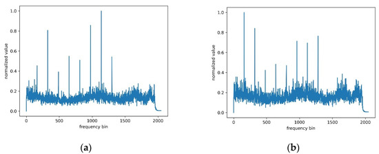
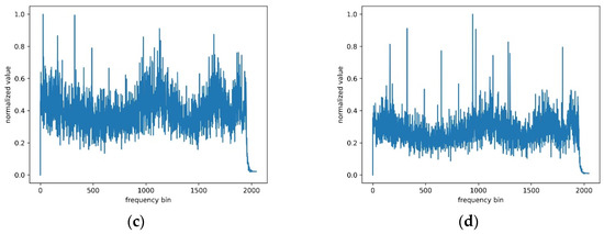
Figure 2.
The DEMON spectrum of different parameters. (a) DEMON spectrums of a reference sample; (b) DEMON spectrums of a sample with Doppler shifts; (c) DEMON spectrums of a sample with low SNR; (d) DEMON spectrums of a sample with interferences.
Dataset A was used for network training, and datasets B, C, and D were used to evaluate the network performance for Doppler shifts, SNRs, and interference. Datasets E, F, and G with 10 types of new targets were used for network performance testing. The detailed information on datasets is shown in Table 1.

Table 1.
The dimensions of datasets A to G.
2.2.2. Generation of Positive and Negative Sample Pairs
A pair of samples was used as training data for a Siamese network. The difference between them was obtained, making it possible to recognize targets from a small sample.
When the sample pairs were from the same target, they were called positive sample pairs. There were 3000 samples in dataset A for each type of target. According to mathematical knowledge, combined formulas can be written as
where is the total number of samples, and represents the number of samples arbitrarily selected from . Positive sample pairs were formed by randomly selecting two samples from the 3000 samples, so the number of positive sample pairs was . The training dataset AA+ for the Siamese network was generated by selecting 7000 random pairs from .
There were 500 samples in datasets B, C, and D for each type. Their positive sample pairs were generated in the same way as dataset A. Consequently, the number of positive sample pairs was , , and . Datasets BB+, CC+, and DD+ were generated by selecting 500 pairs for NB+, NC+, and ND+.
In the same way as datasets B, C, and D, the number of positive sample pairs for datasets E, F, and G were , , and , respectively. Datasets EE+, FF+, and GG+ were generated by selecting 1000 pairs for each type.
Similarly, when the sample pairs were from different targets, they were called negative sample pairs. Datasets AA−, BB−, CC−, DD−, EE−, FF−, and GG− were generated by the same method.
Positive sample pairs were labeled “1”, and negative sample pairs were labeled “0.” The numbers of positive and negative sample pairs for training, validation, and testing are shown in Table 2.
Table 2.
The dimensions of positive and negative sample pairs.
3. Design of the Siamese Network
Siamese networks can evaluate the similarity between two samples and are based on metric learning. Unlike traditional machine learning schemes, Siamese networks can recognize new targets from a small sample after being trained by a large number of other samples [26].
The architecture of the proposed Siamese network is shown in Figure 3 and has two parts. One is feature extraction, which consists of two convolutional neural networks (CNNs) with shared weights. Compared to recurrent neural networks (RNN) and artificial neural networks (ANN), since the feature detection layer of CNN learns through the training data, it learns implicitly from the training data. CNN is more suitable for UATR. When evaluating network performance, in order to understand it more comprehensively, an MLP network was designed to be compared with CNN. The other part is a similarity calculator, which calculates the Euclidean distance between the two outputs of the Siamese sub-networks. Samples X1 and X2 are an input sample pair, which can be positive or negative. The output indicates the difference between the two samples.
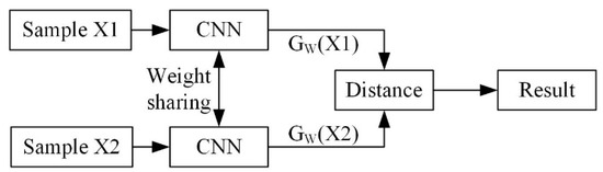
Figure 3.
Siamese network architecture.
The Euclidean distance between two samples can be written as
where is the eigenvector of sample , is the eigenvector of sample , and represents the similarity between sample and sample . In principle, the larger is, the less the similarity between samples and ; the smaller is, the more the similarity [27].
Next, the Siamese network is trained using a contrastive loss function to extract differentiated features. Raia Hadsell et al. first proposed the contrastive loss function to determine whether two inputs were positive or negative [28].
A dataset with sample pairs is , where is the sample pair and is the label of the sample pair. If the sample pair was positive, ; otherwise, . The contrastive function is expressed as
where is the Euclidean distance, and margin is the threshold. According to (10), d is minimized if samples and are a positive pair and maximized if and are a negative pair. This makes the differences between the extracted features more significant.
A CNN is a feed-forward neural network often employed in image feature extraction and classification [29]. The architecture of the Siamese network proposed in this paper is shown in Figure 4. Network parameters, such as convolution layers and kernels, were all optimized by exhaustive search.
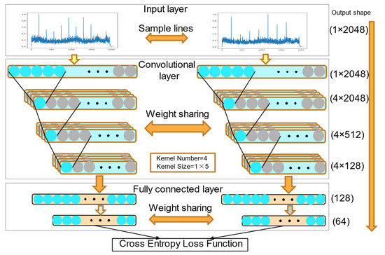
Figure 4.
The proposed Siamese network architecture.
In this study, the inputs of the two identical sub-networks were a pair of samples, each with 2048 × 1 data. More specifically, through multiple convolutions, pooling, and fully connected inputs, output vectors were obtained to calculate the Euclidean distance, and the contrastive loss function determined whether the input pair was positive.
The Siamese network with CNN had three convolution layers, with four convolution kernels per layer. The size of convolution kernels was five. The output parameters and dimensions of each layer are shown in Table 3.
Table 3.
The parameters of the proposed Siamese network with CNN.
When evaluating network performance, in order to understand it more comprehensively, an MLP network was designed to be compared with 1D-CNN. When the complexity of the network reached a certain level, the increase in the number of layers was not helpful for performance improvement. Considering that a simple structure reduces the number of calculations for network propagation, the structural parameters of the MLP listed in Table 4 were finally selected.
Table 4.
The parameters of the proposed Siamese network with MLP.
4. Experiments and Results
4.1. Network Training
Before training the network, all parameters were initialized using Glorot initialization. The rectified linear unit (ReLU) [30] was the activation function for each convolutional layer. The batch size was 128, the training epoch was 20, and the network parameters were optimized by the Adam optimization algorithm. Sample pairs were input to the two sub-networks to obtain feature vectors of the same dimension. We could determine whether a sample pair was positive by calculating the Euclidean distance of output vectors and comparing it with the threshold.
After training the Siamese network with dataset AA and evaluating the performance with datasets BB, CC, and DD, the network parameters were tuned. The optimized parameters of the Siamese network are shown in Table 3.
4.2. Network Performance Test
Datasets EE, FF, and GG were used to test the performance of the Siamese network to recognize new targets with different parameters.
- Performance evaluation of Doppler shifts.
Dataset EE was used to assess the performance of the Siamese network to recognize new targets with different Doppler shifts. Positive and negative sample pairs were input to test the network accuracy for moving targets with different velocities. The results are shown in Figure 5. The horizontal axis is the relative Doppler shift [31], and the vertical axis is the accuracy of the Siamese network.
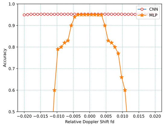
Figure 5.
The performance of the proposed Siamese network for Doppler shifts.
Figure 5 shows the high accuracy of the network for 10 types of new targets and 41 Doppler shifts. The result shows that the proposed network with CNN can recognize new targets with different Doppler shifts. The recognition rate of the Siamese network with MLP is relatively low.
To further evaluate the recognition performance with dataset EE, we analyzed the results of samples with the maximum relative Doppler shift (fd = 0.02). The classification results are shown in Figure 6, where the vertical axis is the actual label, and the horizontal axis is the predicted label. There are 10 types of targets, and the number of samples in each type is 1000. The color depth reflects the accuracy of recognition.
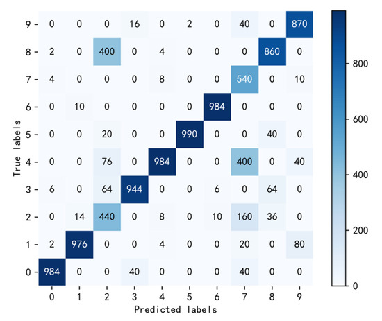
Figure 6.
The classification results of samples with fd = 0.02.
Precision [32] is defined here as the probability of being a positive sample among all predicted positive samples, which can be expressed as
“Recall” [33] is the probability of being predicted as a positive sample among the actual positive samples, which can be expressed as
where n is the sample label of the n-th type, TP represents true positive, FP denotes false positive, and FN is false negative.
We introduced a new measure of balance between them: the F1-score [34]. The F1-score considered both the precision rate and the recall rate so that the two can reach their maxima simultaneously and achieve a balance. The F1-score is expressed as
By calculating the average F1-score of each type, F1average can be written as
where N is 10.
When the Doppler shift (fd = 0.02) was at maximum, the calculated value of F1average was 0.8462.
- Performance evaluation of SNRs.
Dataset FF was used to evaluate the performance of the Siamese network to recognize new targets with 16 types of SNRs. Positive and negative sample pairs were input to the network to assess the accuracy of the network for targets with different SNRs. The results of the evaluation are shown in Figure 7. The horizontal axis is the factor that controls the SNR, and the vertical axis is the accuracy of the network.
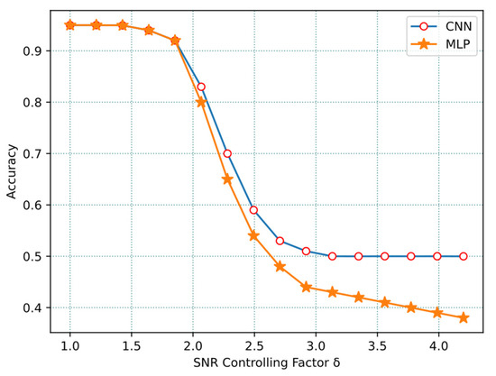
Figure 7.
The performance of the proposed Siamese network for SNRs.
As shown in Figure 7, the Siamese network has a high accuracy for 10 types of new targets and 16 SNRs when . As μ increase, the accuracy of the network decreases rapidly, but it remains above 80% for . Experiments showed that when the SNR is within a certain range, the network with CNN identifies underwater targets accurately. The recognition rate of the Siamese network with MLP is relatively low.
The classification results for when μ was 2.2 are shown in Figure 8. The calculated value of F1average was 0.6403 using the same method.
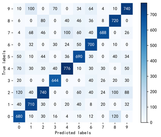
Figure 8.
Classification result of samples with μ = 2.2.
- Performance evaluation of interference.
Dataset GG was used to evaluate the performance of the Siamese network in recognizing new targets with different levels of interference. Positive and negative sample pairs were input to the network to assess the accuracy of the network for targets with different parameters. The results of the evaluation are shown in Figure 9. The horizontal axis shows the number of interference occurrences (negative data indicate the loss of line spectra), and the vertical axis shows the accuracy of the network.
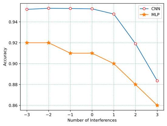
Figure 9.
The performance of the proposed Siamese network for interferences.
As shown in Figure 9, our proposed network identifies targets well with various interference levels. Experiments showed that the network could accurately identify underwater targets when the number of line spectra increased or decreased within a certain range. The recognition rate of the Siamese network with MLP was relatively low.
The classification results when the number = 2 are shown in Figure 10. The calculated F1average was 0.7423 using the same method.
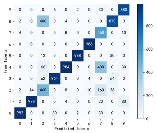
Figure 10.
The classification results of samples with number = 2.
5. Conclusions
Due to the high cost of underwater target data acquisition, a Siamese network for identifying DEMON spectra of underwater targets was developed during our study and reported in this paper. We used the simulation data to train and evaluate the network performance and then used the simulating and real samples to test the network performance; then, we added more real samples to evaluate the network performance. The proposed network recognized targets accurately from a small sample. During the training process, the parameters of the Siamese network were tuned by evaluating datasets with different Doppler shifts, SNRs, and interference to obtain a network with good generalization performance. The article did not study the underwater target radiation noise deeply enough, and the difference between the virtual sample obtained from simulation and the real sample will cause the network recognition performance to be affected. The research of underwater target radiation noise modeling should be strengthened to reduce the differences between the simulated samples and the real samples. On the other hand, the number of real target samples increased in the network training process to improve the network recognition performance. The experimental results showed that a network trained on samples without a Doppler shift and interference has a high Doppler tolerance and can recognize underwater targets with different SNRs and levels of interference. The cross-entropy contrastive loss function enabled the differences between input sample pairs to be determined accurately so that targets can be recognized from small samples. Convolutional neural networks need a large number of training samples to achieve the ideal recognition effect, although the twin network-based small sample UATR algorithm effectively improves the recognition accuracy of the algorithm in the case of insufficient training samples; however, improving the recognition rate of the UATR algorithm in the case of very few underwater target samples or even a single sample is the next problem to be seriously considered.
The approach mentioned in this paper differs from the traditional approach of using a large number of multi-state samples to train the network and then to identify multi-state samples. In this paper, we used single-state samples to train the network, and the results showed that we can better identify multi-state samples. In this paper, more simulation samples were used for evaluation and fewer real samples were used for testing. For our next study, we will evaluate the network with more real samples so that the new real samples will be identified with better results. If necessary, all simulation samples for training and evaluation will be replaced with real samples. This study needs to be completed on the basis of subsequent collection of a sufficient amount of real data. In addition, the cpu-based UATR is slow, and we will port the network model to FPGA for accelerated recognition. The training and recognition rate of the network model for a large number of samples can be greatly improved by the ARM architecture.
Author Contributions
Conceptualization, D.L.; methodology, D.L., W.S. and W.C.; software, formal analysis, W.H., B.W. and W.S.; validation, W.S. and W.C.; writing—original draft preparation, W.H. and B.W.; writing—review and editing, W.S. and W.C.; supervision, D.L.; project administration, D.L. All authors have read and agreed to the published version of the manuscript.
Funding
This research was funded by the Science and Technology Program of Tianjin, grant number 21YDTPJC00180, and the Science and Technology Program of Hebei, grant number 22350901D.
Institutional Review Board Statement
Not applicable.
Informed Consent Statement
Not applicable.
Data Availability Statement
Not applicable.
Conflicts of Interest
The authors declare no conflict of interest.
References
- Hemminger, T.L.; Pao, Y.-H. Detection and classification of underwater acoustic transients using neural networks. IEEE Trans. Neural Netw. 1994, 5, 712–718. [Google Scholar] [CrossRef]
- Yang, H.; Shen, S.; Yao, X.; Sheng, M.; Wang, C. Competitive Deep-Belief Networks for Underwater Acoustic Target Recognition. Sensors 2018, 18, 952. [Google Scholar] [CrossRef]
- Zhu, J.; Christensen, J.; Jung, J.; Martin-Moreno, L.; Yin, X.; Fok, L.; Zhang, X.; Garcia-Vidal, F.J. A holey-structured metamaterial for acoustic deep-subwavelength imaging. Nat. Phys. 2011, 7, 52–55. [Google Scholar] [CrossRef]
- Henclik, S. Underwater acoustic target tracking with fixed passive sonar system. In Proceedings of the 6th European Conference on Underwater Acoustics (ECUA 2002), Gdansk, Poland, 24–27 June 2002. [Google Scholar]
- Zhang, Y.; Sun, J.; Zhang, Y. Research on acoustic signal detection simulation for passive sonar. In Proceedings of the 2010 International Conference on Computational and Information Sciences (ICCIS 2010), Chengdu, China, 17–19 December 2010. [Google Scholar]
- Feng, S.; Zhu, X. A Transformer-Based Deep Learning Network for Underwater Acoustic Target Recognition. IEEE Geosci. Remote Sens. Lett. 2022, 19, 1–5. [Google Scholar] [CrossRef]
- Yao, j.; Wang, D.; Hu, H.; Xing, W.; Wang, L. ADCNN: Towards learning adaptive dilation for convolutional neural networks. Pattern Recognit. 2022, 123, 108369. [Google Scholar] [CrossRef]
- Chen, Z.; Li, Y.; Liang, H.; Yu, J. Hierarchical Cosine Similarity Entropy for Feature Extraction of Ship-Radiated Noise. Entropy 2018, 20, 425. [Google Scholar] [CrossRef]
- Zeng, D.; Peng, R.; Jiang, C.; Li, Y.; Dai, J. CSDM: A context-sensitive deep matching model for medical dialogue information extraction. Inf. Sci. 2022, 607, 727–738. [Google Scholar] [CrossRef]
- Dubey, S.R.; Chakraborty, S. Average biased ReLU based CNN descriptor for improved face retrieval. Multimed. Tools Appl. 2021, 80, 23181–23206. [Google Scholar] [CrossRef]
- Zhu, J.; Hu, T.; Jiang, B.; Yang, X. Intelligent bearing fault diagnosis using PCA-DBN framework. Neural Comput. Appl. 2020, 32, 10773–10781. [Google Scholar] [CrossRef]
- Yang, H.; Li, L.-L.; Li, G.-H.; Guan, Q. A novel feature extraction method for ship-radiated noise. Def. Technol. 2022, 18, 604–617. [Google Scholar] [CrossRef]
- Safi, M.E.; Abbas, E.I. Isolated word recognition based on PNCC with different classifiers in a noisy environment. Appl. Acoust. 2022, 195, 108848. [Google Scholar] [CrossRef]
- Patil, A.A.; Patil, C.B.; Mahulikar, P.P. Effect of coactive influence of LDHs and PNCC on thermal and mechanical properties of epoxy resin. Plast. Rubber Compos. 2021, 50, 209–218. [Google Scholar] [CrossRef]
- Patil, A.A.; Patil, C.B.; Mahulikar, P.P. Impact of synergism of LDH with PNCC on the thermal and mechanical properties of polyester nanocomposites. Polym. Plast. Technol. Mater. 2020, 59, 864–873. [Google Scholar] [CrossRef]
- Zhang, Q.; Bai, J.; Xu, F. A retrieval method for encrypted speech based on improved power normalized cepstrum coefficients and perceptual hashing. Multimed. Tools Appl. 2022, 81, 15127–15151. [Google Scholar] [CrossRef]
- Takacs, B.; Doczi, R.; Suto, B.; Kallo, J.; Varkonyi, T.A.; Haidegger, T.; Kozlovszky, M. Extending AUV Response Robot Capabilities to. Solve Standardized Test Methods. Acta Polytech. Hung. 2016, 13, 157–170. [Google Scholar]
- Bereketli, A.; Tumcakir, M.; Yeni, B. P-AUV: Position aware routing and medium access for ad hoc AUV networks. J. Netw. Comput. Appl. 2019, 125, 146–154. [Google Scholar] [CrossRef]
- Ssegey, Z.; Nikos, K. Learning to Compare Image Patches via Convolutional Neural Networks. In Proceedings of the 2015 IEEE Conference on Computer Vision and Pattern Recognition (CVPR), Boston, MA, USA, 7–12 June 2015. [Google Scholar]
- Yuan, J.; Guo, H.; Jin, Z.; Jin, H.; Zhang, X.; Luo, J. One-shot Learning for Fine-grained Relation Extraction via Convolutional Siamese Neural Network. In Proceedings of the 2017 IEEE International Conference on Big Data (Big Data), Boston, MA, USA, 11–14 December 2017. [Google Scholar]
- Lee, D.-H. One-Shot Scale and Angle Estimation for Fast Visual Object Tracking. IEEE Access 2019, 7, 55477–55484. [Google Scholar] [CrossRef]
- Salberg, A.-B.; Swami, A. Doppler and frequency-offset synchronization in wideband OFDM. IEEE Trans. Wirel. Commun. 2005, 4, 2870–2881. [Google Scholar] [CrossRef]
- Yang, T.; Yang, W. Performance analysis of direct-sequence spread-spectrum underwater acoustic communications with low signal-to-noise-ratio input signals. J. Acoust. Soc. Am. 2008, 123, 842–855. [Google Scholar] [CrossRef]
- Tian, P.; Kang, R.; Yu, H.; Wu, Y. Analysis of quantisation noise within signal band for sinusoidal signal. IET Commun. 2013, 7, 335–339. [Google Scholar] [CrossRef]
- Wu, Y.; Yang, Y.; Yang, L.; Wang, Y. Underwater target recognition based on constant-beamwidth waveform fidelity and interference-suppression. J. Northwestern Polytech. Univ. 2015, 33, 843–848. [Google Scholar]
- Tanveer, M.; Tan, H.K.; Ng, H.F.; Leung, M.K.; Chuah, J.H. Regularization of Deep Neural Network with Batch Contrastive Loss. IEEE Access 2021, 9, 124409–124418. [Google Scholar] [CrossRef]
- Akritas, P.; Antoniou, I.; Ivanov, V.V. I dentification and prediction of discrete chaotic maps applying a Chebyshev neural network. Chaos Solitons Fractals 2000, 11, 337–344. [Google Scholar] [CrossRef]
- Ma, X.; Zhang, S.; Sun, J.; Han, Y.; Du, J.; Fu, X.; Yang, Y.; Sa, Y.; Li, Q.; Yang, C. A TFA-CNN method for quantitative analysis in infrared spectroscopy. Infrared Phys. Technol. 2022, 126, 104329. [Google Scholar] [CrossRef]
- Deng, M.; Zhang, Q.; Zhang, K.; Li, H.; Zhang, Y.; Cao, W. A Novel Defect Inspection System Using Convolutional Neural Network for MEMS Pressure Sensors. J. Imaging 2022, 8, 268. [Google Scholar] [CrossRef]
- Yang, L.; Yang, L.; Ho, K.C. Moving Target Localization in Multistatic Sonar by Differential Delays and Doppler Shifts. IEEE Signal Process. Lett. 2016, 23, 1160–1164. [Google Scholar] [CrossRef]
- Hammad, I.; Li, L.; El-Sankary, K.; Snelgrove, W.M. CNN Inference Using a Preprocessing Precision Controller and Approximate Multipliers with Various Precisions. IEEE Access 2021, 9, 7220–7232. [Google Scholar] [CrossRef]
- Li, M.T.; Lee, S.H. A Study on Small Pest Detection Based on a CascadeR-CNN-Swin Model. CMC Comput. Mater. Contin. 2022, 72, 6155–6165. [Google Scholar] [CrossRef]
- Goncalves, C.B.; Souza, J.R.; Fernandes, H. CNN architecture optimization using bio-inspired algorithms for breast cancer detection in infrared images. Comput. Biol. Med. 2022, 142, 105205. [Google Scholar] [CrossRef]
- DeVries, Z.; Locke, E.; Hoda, M.; Moravek, D.; Phan, K.; Stratton, A.; Phan, P. Using a national surgical database to predict complications following posterior lumbar surgery and comparing the area under the curve and F1-score for the assessment of prognostic capability. Spine J. 2021, 21, 1135–1142. [Google Scholar] [CrossRef]


Publisher’s Note: MDPI stays neutral with regard to jurisdictional claims in published maps and institutional affiliations. |
© 2022 by the authors. Licensee MDPI, Basel, Switzerland. This article is an open access article distributed under the terms and conditions of the Creative Commons Attribution (CC BY) license (https://creativecommons.org/licenses/by/4.0/).