A New Multi-Objective Optimization Design Method for Directional Well Trajectory Based on Multi-Factor Constraints

Abstract

The design of the wellbore trajectory directly affects the construction quality and efficiency of drilling. A good wellbore trajectory is conducive to guiding on-site construction, which can effectively reduce costs and increase productivity. Therefore, further optimization of the wellbore trajectory is inevitable and necessary. Based on this, aiming at the three-segment, five-segment, double-increase-profile extended reach wells, this paper considered the constraints of formation wellbore stability; formation strength; and the determination of the deviation angle, deviation point position, and target range by the work of deflecting tools. In addition, the optimization objective function of the shortest total length of the wellbore, minimum error of the second target, lowest cost, minimum friction of the lifting and lowering string, and minimum torque of rotary drilling were proposed and established. The objective function of the longest extension limit of the horizontal section of the extended reach well is established. Taking the 14-8 block of the Lufeng Oilfield in the eastern South China Sea as an example, the actual data of the field were modeled, and the independence of the objective function was verified by comparing the number of non-inferior solutions of the two objective functions. By normalizing simplified to double-, three-, and four-objective functions, using a genetic algorithm and particle swarm optimization results, it can be found that the new method of optimization design established in this paper has an obvious optimization effect compared with the original design.

1. Introduction

Compared with vertical wells, directional drilling can more flexibly drill target reservoirs [1], pass through more reservoirs, and exploit oil and gas resources that are not easy to develop by conventional means. The design of the borehole track is the key and basic link in the early drilling work, which directly affects the quality and efficiency of subsequent construction [2]. However, the results obtained from the well trajectory design are not certain to be the optimal well trajectory or trajectory to be drilled. Poor well trajectory makes it difficult to control well trajectory, which may lead to serious accidents such as a stuck bit or difficulty applying weight on the bit. Wellbore trajectory optimization is a nonlinear, constrained mathematical optimization problem, which is used to construct an economical, safe, and easily accessible trajectory. The perfect wellbore trajectory optimization can make the track length relatively short while meeting the requirements of field tool capabilities to achieve the goal of reducing working time and saving costs. A suitable hole drift angle can improve the safety factor of the shaft wall. The appropriate angle change rate can make the wellbore slip and benefit safe production. Small torque and friction resistance can reduce the failure rate of drilling tools. Reducing the target error can meet the development requirements of this oilfield [3].

Many optimization algorithms have emerged with the development of computers for decades. Scholars in the field of drilling have applied this optimization to the optimization of well trajectory [4,5,6]. Helmy M.W. et al. (1998) [7] established the objective function of the minimum drilling depth and the constraints of geometric parameters for the semi-S-shaped wellbore trajectory and used the penalty function method to conduct numerical solutions. Jiang Shengzong et al. (1999) [8] proposed a new method for designing 3D trajectory in sidetracking horizontal wells based on optimization theories, which include some factors such as kickoff point, performances of bent housing motors, and tool-face angles. Zhang et al. (1999) [9] established the shortest objective function of the wellbore trajectory length for directional well drilling and proposed the SUM hybrid optimization method. Sui Mancang et al. (2000) [10] set up the objective function of the shortest length of the well track and the constraint conditions such as flexion and strength for the well track of horizontal wells and numerically solved them by using the discrete optimization method. Liu (2001) [11] constructed the shortest well track length objective function and simple geometric constraint conditions for the well track of two-dimensional three-section, five-section, and double-increment-section profiles. The three-dimensional analysis of the wellbore trajectory is carried out, and the penalty function method is used to numerically solve it. Yu et al. (2003) [12] instituted nonlinear equations of borehole trajectory parameters for three-dimensional orbits and proposed the use of the numerical optimization method to numerically solve them. Liu et al. (2004) [13] fathered the objective function of minimum friction resistance for tripping of the drill string and used the Ritz and multidimensional optimization methods for numerical solution. Shokir et al. (2004) [14] established the objective function of the shortest length of borehole trajectory for a seven-section three-dimensional trajectory and used a genetic algorithm to numerically solve it. Lu (2005) [15] found three-dimensional multitarget coordinate incremental equations and proposed the objective function of the shortest well orbit length and the numerical optimization method. Yan et al. (2007) [16] built the objective function with the lowest track cost for the stepped horizontal well and used the external penalty function method for the numerical solution. Sun (2013) [17] constructed the objective function and geometric constraint conditions of the shortest track length, highest target accuracy, lowest drilling cost, and minimum friction resistance of the string for the horizontal well with a two-dimensional double-increase profile, and used the artificial fish swarm optimization method for the numerical solution. Jia et al. (2014) [18] instituted objective functions of the wellbore length, friction resistance, and torque, as well as simple geometric constraints for the modified catenary wellbore trajectory of a 3D triple-increment profile; normalized multiple objective functions into single objective functions through linear weighting; and optimized solutions by using the tolerance method. Atashnezhad A. et al. (2014) [19] established the objective function of the measured depth and actual vertical depth of a borehole orbit for a seven-section three-dimensional orbit and used the new particle swarm optimization algorithm for the numerical solution. Mansouri V. et al. (2015) [20] set up the dual objective function and geometric constraint conditions for the minimum depth of well track measurement and the minimum drilling torque for the seven-section three-dimensional trajectory, and used the multi-objective genetic algorithm method for the numerical solution. Gao et al. (2019) [21] used the vector algebra method and minimum curvature method to solve the trajectory design problem of the intersection of two wells. Wood (2016) [22], Wang (2016) [23], Sha (2018) [24], Huang (2018) [25], Khosravanian (2018) [26], Li (2019) [27], Zhen (2019) [28], and Wang et al. (2020) [29] also carried out relevant studies on three-dimensional orbit.

For the problem of well trajectory optimization, the existing methods often take a single target as the research object, and the research on the problem of well trajectory to target optimization is less. At the same time, most of them take the minimum friction and the shortest well length as the objective function without considering the target accuracy and other optimization objectives. Concurrently, some optimization algorithms are used to obtain local optimal solutions. In this paper, various optimization algorithms [30,31] were selected in the investigation; and, combined with the existing conditions, the formation wellbore stability, formation strength, and work of the deflection tool are considered to carry out a combination of multiple factors to achieve the trajectory optimization research; moreover, the borehole trajectory optimization method is established with multiple objective functions, such as wellbore trajectory length, target error, friction torque, open-hole extension limit, etc. Compared with the previous studies, more comprehensive factors were considered and more objective functions were established in this paper.

2. Optimization Model

2.1. Well Track Length

Common calculation methods of two-dimensional borehole trajectory mainly include the arc model, catenary model, parabola model, cycloid model, etc. [32,33,34]. The arc line model assumes that the rate of deviation change remains unchanged on the track length, which is convenient for trajectory control. Therefore, it is assumed that the well track is composed of a straight line segment and an arc line segment.

The arc line model of the build-up section is shown in Figure 1, and the calculation model is [35]

$${\alpha }_2={\alpha }_1+k\Delta L={\alpha }_1+\frac{180}{\pi }\cdot \frac{\Delta L}{R}$$

(1)

$$\Delta H=R\left(\sin {\alpha }_2-\sin {\alpha }_1\right)$$

(2)

$$\Delta S=R\left(\cos {\alpha }_1-\cos {\alpha }_2\right)$$

(3)

where ΔL, ΔH, and ΔS are, respectively, the well track length, vertical depth increase, and horizontal length increase of point B relative to the initial point A of deflecting, m. R is the radius of the build-up section. In order to reduce annular pressure loss and operation time of drilling before the target, the well track length before the target should be minimized. Then, the minimum objective function of the well track length can be expressed as follows:

$$\min L=\min {\displaystyle \sum _{i=1}^n{L}_i}$$

(4)

2.2. Cost of Drilling

In order to minimize the cost of drilling operations in front of the target point, it is assumed that the drilling costs of the vertical well and angle maintaining sections and the build-up and drop-off sections are, respectively, C₁ and C₂ 10,000 CNY/h, ignoring the equipment costs of the drill bit and string and the labor and fuel operating costs. Then the lowest objective function of drilling cost C can be expressed as

$$\min C=\min \left(\frac{C_1}{v_i}{\displaystyle \sum _{i=1}^n{L}_i}+\frac{C_2}{v_j}{\displaystyle \sum _{j=1}^k{L}_j}\right)$$

(5)

where $v_i$ and $v_j$ are the ROP (rate of penetration) of the well section, m/h; $L_i$ and $L_j$ are the track lengths of the well section, m.

2.3. Target Error of First Target

The target accuracy of the directional well is the early guarantee of drilling into oil reservoirs; especially for reservoirs with small range, accurate crossing of the target is particularly important. When the position of the first target coincides with the coordinates, the error of the target is minimum. Then, the objective function of the minimum target error can be expressed as

$$\min \delta =\min \left\{{\left[{\left({\left(X_{T^{\prime }}-X_O\right)}^2+{\left(Y_{T^{\prime }}-Y_O\right)}^2\right)}^{0.5}-S_{T^{\prime }}\right]}^2+{\left(Z_T-Z\right)}^2\right\}$$

(6)

where O($X_O$,$Y_O$,$Z_O$) is the center coordinate of the wellhead; T′($X_T$,$Y_T$,$Z_{T^{\prime }})$ are the coordinates of the first target; T($X_T$,$Y_T$,$Z_T)$ are the coordinates of the second target; $S_{T^{\prime }}$ is the horizontal projection displacement of the first target obtained, m; and Z is the relative vertical depth of the decision variable reaching the first target, m.

2.4. Friction

It is assumed that the support of the borehole wall to the drill-string is rigid; the drill-string elastic deformation line completely coincides with the well axis, ignoring the weight on the bit. Assuming that the bending section is divided into 500 equal parts, the expression of the well inclination angle of the microelement section is given below:

(1)

Hold section

Figure 2 shows the stress analysis of the element string in the hold section. The axial stress balance relation of the microelement section is as follows:

$$T_{i+1}=T_i\pm \mu N\left(L_{i+1}-L_i\right)+q\left(L_{i+1}-L_i\right)\cos \alpha$$

(7)

where $T_{i+1}$ and $T_i$ are the axial forces at the upper and lower ends, respectively, of the i-section string unit, N; “±” is “+” in the process of lifting and is “−” in the process of lowering; μ is the sliding friction coefficient between the pipe string and the pipe wall, and is dimensionless; $L_{i+1}$ and $L{ }_i$ are, respectively, the measured depths at both ends of the i-section string unit, m; q is the line weight of the string, N/m; and α is the well inclination angle. The radial force balance relation is

$$N=q\sin \alpha$$

(8)

Then the expression of friction force in this element segment is

$$F=\mu q\cos \alpha$$

(9)

(2)

Build-up section

Figure 3 shows the stress analysis of the build-up section unit string. According to [36], the axial force of the microsegment can be deduced as follows:

$$T_{i+1}=\left(T_i\mp A\sin {\beta }_i-B\cos {\beta }_i\right)e^{\mp \mu \left({\beta }_{i+1}+{\beta }_i\right)}\pm A\sin {\beta }_{i+1}+B\cos {\beta }_{i+1}$$

(10)

$$A=\frac{2\mu }{1+{\mu }^2}qR,B=\frac{{\mu }^2-1}{{\mu }^2+1}qR$$

(11)

where “∓” is “−” when N > 0 or is “+” when N < 0 in the process of lifting, and is “+” when N > 0 or is “−” when N < 0 in the process of lowering; “±” is “+” when N > 0 or is “−” when N < 0 in the process of lifting, and is “−” when N > 0 or is “+” when N < 0 in the process of lowering; and ${\beta }_{i+1}$ and ${\beta }_i$ are the residual angles of the upper and lower ends of the I string unit, respectively. The expression of frictional force in the microsegment is

$$F_i=\pm T_{i+1}\mp T_i\pm qR\left(\cos {\beta }_{i+1}-\cos {\beta }_i\right)$$

(12)

where “±” is “+” in the process of lifting and is “−” in the process of lowering; “∓” is “−” in the process of lifting and is “+” in the process of lowering.

(3)

Drop-off section

Figure 4 shows the stress analysis of the build-off section unit string. According to [36], the axial force of the microsegment can be deduced as follows:

$$T_{i+1}=\left(T_i\pm A\sin {\alpha }_i+B\cos {\alpha }_i\right)e^{\pm \mu \left({\alpha }_{i+1}+{\alpha }_i\right)}\mp A\sin {\alpha }_{i+1}-B\cos {\alpha }_{i+1}$$

(13)

where “±” is “+” in the process of lifting and is “−” in the process of lowering; “∓” is “−” in the process of lifting and is “+” in the process of lowering. The expression of frictional force in the microsegment is

$$F_i=\pm T_{i+1}\mp T_i\mp qR\left(\sin {\alpha }_{i+1}-\sin {\alpha }_i\right)$$

(14)

In order to reduce the drilling difficulty, friction should be minimized as far as possible. The minimum friction objective function in the process of lifting or lowering the string in front of the target can be expressed as

$$\min F=\min \left[\mu q{\displaystyle \sum _{i=1}^j\left(L_i\sin {\alpha }_i\right)}+{\displaystyle \sum _{i=1}^n{F}_i}\right]$$

(15)

2.5. Torque

(1)

Hold section

$$M_{i+1}=M_i+\mu q\sin \alpha \left(L_{i+1}-L_i\right)D_t/2$$

(16)

where $D_t$ is the diameter of the pipe string, mm.

(2)

Build-up section

The expressions of the axial force and torque for the microelement segment ignoring sliding friction are

$$T_{i+1}=T_i+qR\left(\cos {\beta }_i-\cos {\beta }_{i+1}\right)$$

(17)

$$M_{i+1}=M_i+\mu \left|q\cos {\beta }_{i+1}-T_{i+1}/R\right|D_t/2000R\left({\beta }_{i+1}-{\beta }_i\right)$$

(18)

(3)

Drop-off section

The expressions of the axial force and torque for the microelement segment ignoring sliding friction are

$$T_{i+1}=T_i+qR\left(\sin {\alpha }_{i+1}-\sin {\alpha }_i\right)$$

(19)

$$M_{i+1}=M_i+\mu \left|q\sin {\alpha }_{i+1}+T_{i+1}/R\right|D_t/2000R\left({\alpha }_{i+1}-{\alpha }_i\right)$$

(20)

In order to reduce the drilling difficulty, torque should be minimized. The minimum objective function of torque for rotary drilling before the target can be expressed as

$$\min M=\min \left[M_0+\mu q{D}_t/2{\displaystyle \sum _{i=1}^j\left(L_i\sin {\alpha }_i\right)}+{\displaystyle \sum _{i=1}^n{M}_i}\right]$$

(21)

2.6. Open-Hole Extension Capability of Extended Reach Wells

For drilling conditions with cuttings considered, the influence factors of the extended reach limit of horizontal wells include annular pressure loss in vertical $\Delta p_v$ and deviated sections ${\displaystyle \sum _{i=1}^j\Delta p_{di}}$ and an annular pressure loss gradient in horizontal sections ${\left(\Delta p/\Delta L\right)}_h$ [37,38,39]. For the extended reach horizontal well, the longer the horizontal section, the better the oil and gas production and economic benefit. The objective function of the maximum horizontal section open-hole extension capacity can be expressed as

$$\max L_h=\max \frac{0.00981\left({\rho }_f-{\rho }_{mix}\right)D_v-\left(\Delta p_v+{\displaystyle \sum _{i=1}^j\Delta p_{di}}\right)}{{\left(\Delta p/\Delta L\right)}_h}$$

(22)

where ${\rho }_{mix}={\rho }_s{C}_s-{\rho }_m\left(1-C_s\right)$; ${\rho }_{mix}$, ${\rho }_s$, and ${\rho }_m$ are, respectively, the density of the solid–liquid mixture, cuttings density, and drilling fluid density, g/cm³; $C_s$ is the solid-phase volume fraction, %.

2.7. Constraints

(1)

The velocity of wellbore trajectory change can be controlled by the build-up rate. When the build-up rate is low, the length of the well orbit required to reach the target increases, thus extending the drilling cycle. When the build-up rate is large, the construction speed is fast, which may lead to stuck bit and increased construction difficulty [40]. The build-up rate should be between the maximum build-up rate and minimum build-up rate of the deflecting tool. For conventional directional wells, the build-up rate is generally (2.1–4.2) (°)/30 m, and the drop-off rate is generally less than 2.5 (°)/30 m [41]. There is a lot of feed for extended reach wells in the inclined section. Controlling the build-up rate below 3 (°)/30 m is beneficial to reduce friction and casing wear and prevent fatigue damage to drilling tools during rotation. The range constraint expression of build-up rate k is shown in Formula (23). In order to prevent track loss and landing, the building slope of the offshore platform is generally (2.5–3) (°)/30 m.

$$k_{\min }\le k\le k_{\max }$$

(23)

(2)

According to the calculation of the safety density window, the stable inclination should be between the maximum stable inclination angle and minimum stable inclination angle under the condition of wellbore stability. According to the law of rock carrying, the inclination angle between 48° and 68° is the most unfavorable to rock carrying. For directional wells, if the angle of inclination is less than 15°, the borehole orientation is unstable and drift is easy to occur. If the deviation value is more than 45°, it is not conducive to wellbore torsion, and logging and completion operations are relatively difficult.

$${\alpha }_{\min }\le \alpha \le {\alpha }_{\max }$$

(24)

(3)

When the stratum strength is low, the dip force generated by the BHA is small, restricting the build-up rate’s rise. When the stratum strength is high, the inclination-building effect of the inclination-building force generated by the bottom hole assembly decreases, which restricts the improvement of the build-up rate. Therefore, it is necessary to combine the formation strength factors to select the location of the inclination-making point, and it should be located in the medium-soft to medium-hard stratum, which is most conducive to the inclination making [42,43]. To establish the constraint conditions considering the influencing factors of formation strength, the uniaxial compressive strength value of formation can be input into the program, and the function of formation strength and vertical depth can be established. Through the program call, the constraint range of formation strength can be determined according to

Table 1. Relation between compressive strength and formation.

Layer	Drillability	Compressive Strength (MPa)
Dead-soft	Level 1–2	<25
Soft	Level 3	25–50
Medium-soft	Level 4	50–75
Medium	Level 4–5	75–100
Medium-hard	Level 5–6	100–150
Hard	Level 5–6	150–200
Extrahard	More than 7	>200

[44], and the appropriate depth can be selected. Then, the expression can be expressed as

$$UC{S}_{\min }\le UCS\left(Z_i\right)\le UC{S}_{\max }$$

(25)

(4)

When the vertical depth of the kickoff point is shallow, the length of the build-up section will be increased,; then the drilling operation cycle will be extended, and the drilling operation will be more difficult. When the vertical depth of the kickoff point is deep, the build-up rate will be increased, thus increasing the difficulty of construction [45]. The constraint expression of the vertical depth range of the first kickoff point is shown in Formula (26). According to the requirements of the offshore cluster well standard, in order to quickly make the surface separation and reduce the risk of collision prevention, the position of the first kickoff point Z_A is generally chosen at one to two pillars after the catheter shoe.

$$h_{\min }\le Z_A\le h_{\max }$$

(26)

(5)

The vertical depth and plane error of the second target should be less than the specified range, and the constraint conditions can be expressed as

$$\{\begin{array}{l}\left|Z-Z_T\right|\le H\hfill \\ \left|S_T-\sqrt{{\left(X_O-X_T\right)}^2+{\left(Y_O-Y_T\right)}^2}\right|\le J\hfill \end{array}$$

(27)

where J is the allowable error in the plane, and H is the allowable error in the vertical.

(6)

In order to prevent errors in program calculation, geometric constraints should be considered, and the length of the steady slope section should not be less than zero. Then, the expression is

$$L_j\ge 0$$

(28)

3. Optimize the Design Model

3.1. Three-Stage

The key points of the well track in Figure 5 are as follows: the wellhead position O, the start point of build-up A, the end point of build-up B, the first target T′, and the second target T.

Let the known parameters be the wellhead center coordinates O($X_O$,$Y_O$,$Z_O$); coordinates of the first target T′($X_{T^{\prime }}$,$Y_{T^{\prime }}$,$Z_{T^{\prime }}$); coordinates of the second target T($X_T$,$Y_T$,$Z_T$); plane allowable error J; vertical allowable error H; vertical depth range of kickoff point A($Z_{Amin}$,$Z_{Amax}$); range of formation strength at kickoff point ($UC{S}_{min}$,$UC{S}_{max}$); range of k build-up rate ($k_{min}$,$k_{max}$); and range of α stable inclination angle (${\alpha }_{min}$,${\alpha }_{max}$).

The decision variables are set as follows: the vertical depth $Z_A$ of the kickoff point A, m; vertical depth Z of the second target, m; stable inclination angle α, (°); and build-up rate k, (°)/30 m.

The integrated well has the shortest track length, lowest drilling cost, minimum target error in the first target, minimum drag in the up and down string, and minimum torque in rotary drilling. The multi-objective optimization function can be expressed as

$$\{\begin{array}{l}\min L_T=\min \left(Z_A+L_{AB}+L_{BT}\right)\\ \min C=\min \left(\frac{C_1}{v_i}{\displaystyle \sum _{i=1}^n{L}_i}+\frac{C_2}{v_j}{\displaystyle \sum _{j=1}^k{L}_j}\right)\\ \min \delta =\min \left\{{\left[{\left({\left(X_{T^{\prime }}-X_O\right)}^2+{\left(Y_{T^{\prime }}-Y_O\right)}^2\right)}^{0.5}-S_{T^{\prime }}\right]}^2+{\left(Z_T-Z\right)}^2\right\}\\ \min F=\min \left(\mu q{L}_{BT}\sin \alpha +{\displaystyle \sum _{i=1}^{500}{F}_i}\right)\\ \min M=\min \left(M_0+\mu q\sin \alpha L_{BT}{D}_t/2+{\displaystyle \sum _{i=1}^{500}\Delta M_i}\right)\end{array}$$

(29)

Considering multiple factors such as formation strength and geometric constraints, the constraint conditions can be expressed as follows:

$$\{\begin{array}{l}{k}_{\min }\le k\le k_{\max }\\ {\alpha }_{\min }\le \alpha \le {\alpha }_{\max }\\ UC{S}_{\min }\le UCS\left(Z_A\right)\le UC{S}_{\max }\\ h_{\min }\le Z_A\le h_{\max }\\ \left|Z-Z_T\right|\le H\\ \left|S_T-\sqrt{{\left(X_O-X_T\right)}^2+{\left(Y_O-Y_T\right)}^2}\right|\le J\\ L_{BT}\ge 0\end{array}$$

(30)

Other supplementary equation conditions are as follows:

$$\{\begin{array}{l}{L}_{AB}=1719/k\cdot \alpha \\ L_{BT}=\left(Z-Z_A-1719/k\cdot \sin \alpha \right)/\cos \alpha \\ S_T=1719/k\cdot \left(1-\cos \alpha \right)+L_{BT}\tan \alpha \\ S_{T^{\prime }}=S_T+\left(Z_{T^{\prime }}-Z_T\right)\tan \alpha \\ {\alpha }_{i+1}={\alpha }_i-\frac{k}{30}\frac{\pi }{180}\frac{L_{AB}}{500}\\ {\beta }_i=2/\pi -{\alpha }_i\\ T_0=q\left(\cos \alpha +\mu \sin \alpha \right)L_{BT}\\ T_{i+1}=\left(T_i\mp A\sin {\beta }_i-B\cos {\beta }_i\right)e^{\mp \mu \left({\beta }_{i+1}+{\beta }_i\right)}\pm A\sin {\beta }_{i+1}+B\cos {\beta }_{i+1}\\ A=1719/k\cdot \frac{2\mu }{1+{\mu }^2}q,B=1719/k\cdot \frac{{\mu }^2-1}{{\mu }^2+1}q\\ F_i=\pm T_{i+1}\mp T_i\pm 1719/k\cdot q\left(\cos {\beta }_{i+1}-\cos {\beta }_i\right)\\ \Delta M_i=\mu \left|q\cos {\beta }_{i+1}-T_{i+1}/\left(1719/k\right)\right|D_t/2000\times 1719/k\left({\beta }_{i+1}-{\beta }_i\right)\end{array}$$

(31)

where “±” is “+” in the process of lifting and is “−” in the process of lowering; “∓” is “−” in the process of lifting and is “+” in the process of lowering.

3.2. Five-Stage

The key points of the well track in Figure 6 are as follows: the wellhead position O; start point of build-up A; end point of build-up B; start point of drop-off C; end point of drop-off D; first target T′; and second target T.

Let the known parameters be the wellhead center coordinates O($X_O$,$Y_O$,$Z_O$); coordinates of the first target T′($X_{T^{\prime }}$,$Y_{T^{\prime }}$,$Z_{T^{\prime }}$); coordinates of the second target T(($X_T$,$Y_T$,$Z_T$); plane allowable error J; vertical allowable error H; vertical depth range of kickoff point A($Z_{Amin}$,$Z_{Amax}$); range of formation strength at kickoff point A($UC{S}_{min}$,$UC{S}_{max}$); range of formation strength at drop-off point C($UC{S}_{min}$,$UC{S}_{max}$); range of k₁ build-up rate ($k_{1min}$,$k_{1max}$); range of k₂ drop-off rate ($k_{2min}$,$k_{2max}$); range of first stable inclination angle ${\alpha }_1$(${\alpha }_{1min}$,${\alpha }_{1max}$); and range of second stable inclination angle ${\alpha }_2$ (${\alpha }_{2min}$,${\alpha }_{2max}$).

The decision variables are set as follows: the vertical depth $Z_A$ of the kickoff point A, m; vertical depth $Z_C$ of the drop-off point C, m; vertical depth Z of the second target, m; first stable inclination angle ${\alpha }_1$, (°); second stable inclination angle ${\alpha }_2$, (°); build-up rate $k_1$, (°)/30 m; and drop-down rate $k_2$, (°)/30 m.

The integrated well has the shortest track length, lowest drilling cost, minimum target error in the first target, minimum drag in the up and down string, and minimum torque in rotary drilling. The multi-objective optimization function can be expressed as

$$\{\begin{array}{l}\min L_T=\min \left(Z_A+L_{AB}+L_{B\mathrm{C}}+L_{CD}+L_{DT}\right)\\ \min C=\min \left(\frac{C_1}{v_i}{\displaystyle \sum _{i=1}^n{L}_i}+\frac{C_2}{v_j}{\displaystyle \sum _{j=1}^k{L}_j}\right)\\ \min \delta =\min \left\{{\left[{\left({\left(X_{T^{\prime }}-X_O\right)}^2+{\left(Y_{T^{\prime }}-Y_O\right)}^2\right)}^{0.5}-S_{T^{\prime }}\right]}^2+{\left(Z_T-Z\right)}^2\right\}\\ \min F=\min \left[\mu q\left(L_{B\mathrm{C}}\sin {\alpha }_1+L_{DT}\sin {\alpha }_2\right)+{\displaystyle \sum _{i=1}^{500}{F}_{1,i}+{\displaystyle \sum _{i=1}^{500}{F}_{2,i}}}\right]\\ \min M=\min \left[M_0+\mu q\left(L_{B\mathrm{C}}\sin {\alpha }_1+L_{DT}\sin {\alpha }_2\right)D_t/2+{\displaystyle \sum _{i=1}^{500}\Delta M_{1,i}+{\displaystyle \sum _{i=1}^{500}\Delta M_{2,i}}}\right]\end{array}$$

(32)

Considering multiple factors such as formation strength and geometric constraints, the constraint conditions can be expressed as follows:

$$\{\begin{array}{l}{k}_{1\min }\le k_1\le k_{1\max }\\ k_{2\min }\le k_2\le k_{2\max }\\ {\alpha }_{1\min }\le {\alpha }_1\le {\alpha }_{1\max }\\ {\alpha }_{2\min }\le {\alpha }_2\le {\alpha }_{2\max }\\ UC{S}_{A\min }\le UCS\left(Z_A\right)\le UC{S}_{A\max }\\ UC{S}_{C\min }\le UCS\left(Z_C\right)\le UC{S}_{C\max }\\ h_{\min }\le Z_A\le h_{\max }\\ \left|Z-Z_T\right|\le H\\ \left|S_T-\sqrt{{\left(X_O-X_T\right)}^2+{\left(Y_O-Y_T\right)}^2}\right|\le J\\ L_{BC}\ge 0\\ L_{DT}\ge 0\end{array}$$

(33)

Other supplementary equation conditions are as follows:

$$\{\begin{array}{l}{L}_{AB}=1719/k_1\cdot {\alpha }_1\\ L_{BC}=\left(Z_C-Z_A-1719/k_1\cdot \sin {\alpha }_1\right)/\cos {\alpha }_1\\ L_{CD}=1719/k_2\cdot \left({\alpha }_1-{\alpha }_2\right)\\ L_{DT}=\left[Z-Z_C-1719/k_2\cdot \left(\sin {\alpha }_1-\sin {\alpha }_2\right)\right]/\cos {\alpha }_2\\ S_T=1719/k_1\cdot \left(1-\cos {\alpha }_1\right)+L_{BC}\tan {\alpha }_1+1719/k_2\cdot \left(\cos {\alpha }_2-\cos {\alpha }_1\right)+L_{DT}\tan {\alpha }_2\\ S_{T^{\prime }}=S_T+\left(Z_{T^{\prime }}-Z_T\right)\tan {\alpha }_2\\ {\alpha }_{1,i+1}={\alpha }_{1,i}-\frac{k_1}{30}\frac{\pi }{180}\frac{L_{AB}}{500},{\beta }_{1,i}=2/\pi -{\alpha }_{1,i},{\alpha }_{1,0}={\alpha }_1\\ {\alpha }_{2,i+1}={\alpha }_{2,i}-\frac{k_2}{30}\frac{\pi }{180}\frac{L_{CD}}{500},{\alpha }_{2,0}={\alpha }_2\\ T_{2,0}=q\left(\cos {\alpha }_2+\mu \sin {\alpha }_2\right)L_{DT}\\ T_{2,i+1}=\left(T_{2,i}\pm A\sin {\alpha }_{2,i}+B\cos {\alpha }_{2,i}\right)e^{\pm \mu \left({\alpha }_{2,i+1}+{\alpha }_{2,i}\right)}\mp A\sin {\alpha }_{2,i+1}-B\cos {\alpha }_{2,i+1}\\ A_2=1719/k_2\cdot \frac{2\mu }{1+{\mu }^2}q,B_2=1719/k_2\cdot \frac{{\mu }^2-1}{{\mu }^2+1}q\\ F_{2,i}=\pm T_{i+1}\mp T_i\mp 1719/k_2\cdot q\left(\sin {\alpha }_{2,i+1}-\sin {\alpha }_{2,i}\right)\\ T_{1,0}=T_{2,500}+q\left(\cos {\alpha }_1+\mu \sin {\alpha }_1\right)L_{BC}\\ T_{1,i+1}=\left(T_{1,i}\mp A\sin {\beta }_{1,i}-B\cos {\beta }_{1,i}\right)e^{\mp \mu \left({\beta }_{{}_{1,i+1}}+{\beta }_{1,i}\right)}\pm A\sin {\beta }_{1,i+1}+B\cos {\beta }_{1,i+1}\\ A_1=1719/k_1\cdot \frac{2\mu }{1+{\mu }^2}q,B_1=1719/k_1\cdot \frac{{\mu }^2-1}{{\mu }^2+1}q\\ F_{1,i}=\pm T_{1,i+1}\mp T_{1,i}\pm 1719/k_1\cdot q\left(\cos {\beta }_{1,i+1}-\cos {\beta }_{1,i}\right)\\ {T^{\prime }}_{2,i+1}={T^{\prime }}_{2,i}+qR\left(\sin {\alpha }_{2,i+1}-\sin {\alpha }_{2,i}\right),{T^{\prime }}_{2,0}=T_0+q\cos {\alpha }_2{L}_{DT}\\ \Delta M_{2,i}=\mu \left|q\sin {\alpha }_{2,i+1}+{T^{\prime }}_{2,i+1}/\left(1719/k_2\right)\right|D_t/2000\times 1719/k_2\cdot \left({\alpha }_{2,i+1}-{\alpha }_{2,i}\right)\\ {T^{\prime }}_{1,i+1}={T^{\prime }}_{1,i}+qR\left(\cos {\beta }_{1,i}-\cos {\beta }_{1,i+1}\right),{T^{\prime }}_{1,0}={T^{\prime }}_{2,500}+q\cos {\alpha }_1{L}_{BC}\\ \Delta M_{1,i}=\mu \left|q\cos {\beta }_{1,i+1}-{T^{\prime }}_{1,i+1}/\left(1719/k_1\right)\right|D_t/2000\times 1719/k_1\cdot \left({\beta }_{1,i+1}-{\beta }_{1,i}\right)\end{array}$$

(34)

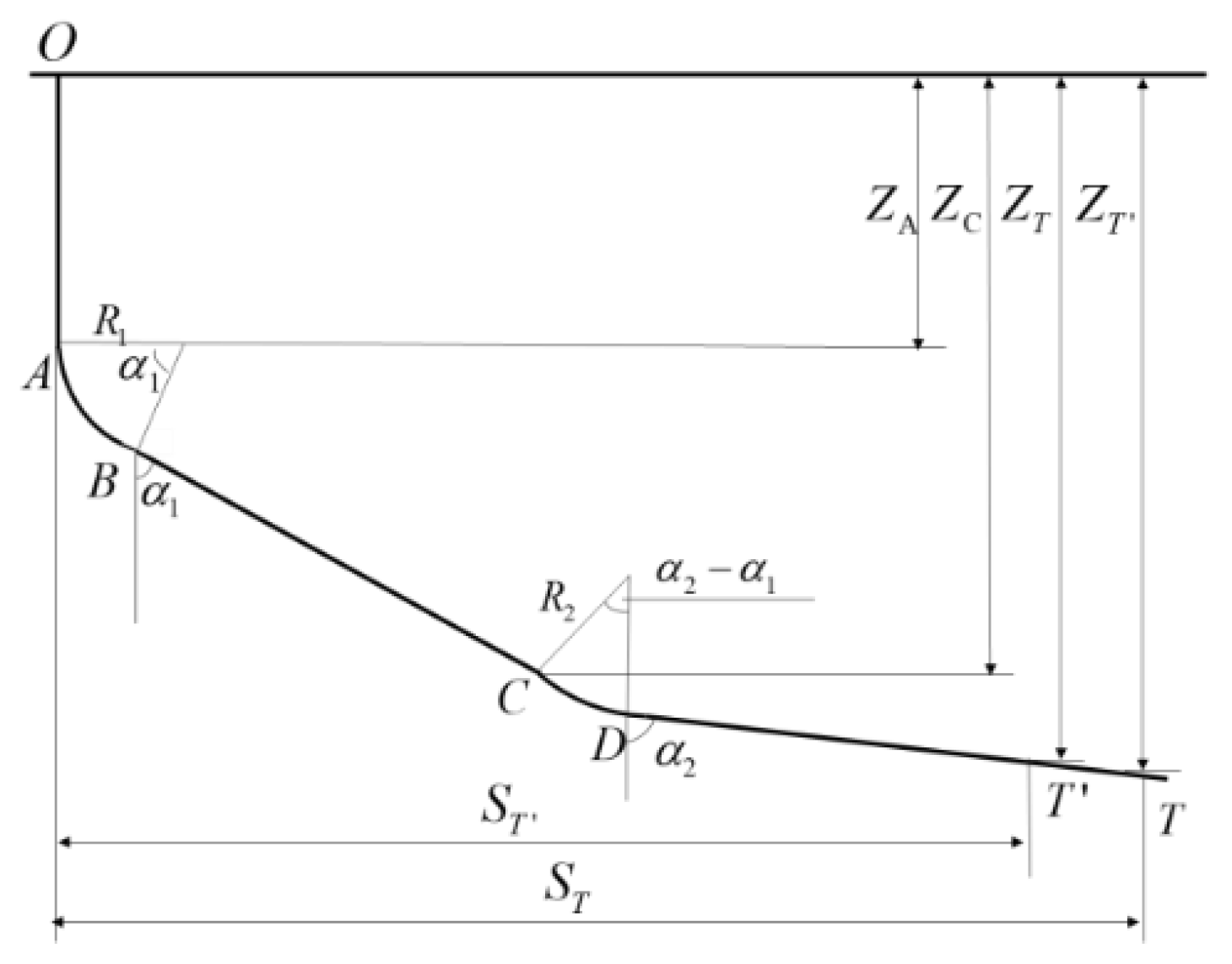
3.3. Extended Reach Well with Double Increasing Profile

The key points of the well track in Figure 7 are as follows: the wellhead position O; first start point of build-up A; first end point of build-up B; second start point of build-up C; second end point of build-up D; first target T′; and second target T.

Let the known parameters be the wellhead center coordinates O($X_O$,$Y_O$,$Z_O$); coordinates of the first target T′($X_{T^{\prime }}$,$Y_{T^{\prime }}$,$Z_{T^{\prime }}$); coordinates of the second target T(($X_T$,$Y_T$,$Z_T$); plane allowable error J; vertical allowable error H; vertical depth range of kickoff point A($Z_{Amin}$,$Z_{Amax}$); range of formation strength at kickoff point A($UC{S}_{min}$,$UC{S}_{max}$); range of formation strength at drop-off point C($UC{S}_{min}$,$UC{S}_{max}$); range of k1 build-up rate ($k_{1min}$,$k_{1max}$); range of k2 drop-off rate ($k_{2min}$,$k_{2max}$); range of first stable inclination angle ${\alpha }_1$(${\alpha }_{1min}$,${\alpha }_{1max}$); and range of second stable inclination angle ${\alpha }_2$(${\alpha }_{2min}$,${\alpha }_{2max}$).

The decision variables are set as follows: the vertical depth $Z_A$ of the kickoff point A, m; vertical depth $Z_C$ of the second kickoff point C, m; vertical depth Z of the second target, m; first stable inclination angle ${\alpha }_1$, (°); second stable inclination angle ${\alpha }_2$, (°); first build-up rate $k_1$, (°)/30 m; and second build-up rate $k_2$, (°)/30 m.

The objective functions of the shortest comprehensive well track length, lowest drilling cost, minimum target error in the first target, minimum drag of the string up or down, minimum torque in rotary drilling, and maximum horizontal open-hole extension capability are as follows:

$$\{\begin{array}{l}\min L_T=\min \left(Z_A+L_{AB}+L_{B\mathrm{C}}+L_{CD}+L_{DT}\right)\\ \min C=\min \left(\frac{C_1}{v_i}{\displaystyle \sum _{i=1}^n{L}_i}+\frac{C_2}{v_j}{\displaystyle \sum _{j=1}^k{L}_j}\right)\\ \min \delta =\min \left\{{\left[{\left({\left(X_{T^{\prime }}-X_O\right)}^2+{\left(Y_{T^{\prime }}-Y_O\right)}^2\right)}^{0.5}-S_{T^{\prime }}\right]}^2+{\left(Z_T-Z\right)}^2\right\}\\ \min F=\min \left[\mu q\left(L_{B\mathrm{C}}\sin {\alpha }_1+L_{DT}\sin {\alpha }_2\right)+{\displaystyle \sum _{i=1}^{500}{F}_{1,i}+{\displaystyle \sum _{i=1}^{500}{F}_{2,i}}}\right]\\ \min M=\min \left[M_0+\mu q\left(L_{B\mathrm{C}}\sin {\alpha }_1+L_{DT}\sin {\alpha }_2\right)D_t/2+{\displaystyle \sum _{i=1}^{500}\Delta M_{1,i}+{\displaystyle \sum _{i=1}^{500}\Delta M_{2,i}}}\right]\\ \max L_h=\max \left[\frac{0.00981\left({\rho }_f-{\rho }_{mix}\right)D_v-\left(\Delta p_v+{\displaystyle \sum _{i=1}^j\Delta p_{di}}\right)}{{\left(\Delta p/\Delta L\right)}_h}\right]\end{array}$$

(35)

Considering multiple factors such as formation strength and geometric constraints, the constraint conditions are similar to the five-stage formula, as shown in Formula (32). Other supplementary equation conditions are as follows:

$$\{\begin{array}{l}{L}_{AB}=1719/k_1\cdot {\alpha }_1\\ L_{BC}=\left(Z_C-Z_A-1719/k_1\cdot \sin {\alpha }_1\right)/\cos {\alpha }_1\\ L_{CD}=1719/k_2\cdot \left({\alpha }_2-{\alpha }_1\right)\\ L_{DT}=\left[Z-Z_C-1719/k_1\cdot \left(\sin {\alpha }_2-\sin {\alpha }_1\right)\right]/\cos {\alpha }_2\\ S_T=1719/k_1\cdot \left(1-\cos {\alpha }_1\right)+L_{BC}\tan {\alpha }_1+1719/k_2\cdot \left(\cos {\alpha }_1-\cos {\alpha }_2\right)+L_{DT}\tan {\alpha }_2\\ S_{T^{\prime }}=S_T+\left(Z_{T^{\prime }}-Z_T\right)\tan {\alpha }_2\\ {\alpha }_{1,i+1}={\alpha }_{1,i}-\frac{k_1}{30}\frac{\pi }{180}\frac{L_{AB}}{500},{\alpha }_{1,0}={\alpha }_1,{\beta }_{1,i}=2/\pi -{\alpha }_{1,i}\\ {\alpha }_{2,i+1}={\alpha }_{2,i}-\frac{k_2}{30}\frac{\pi }{180}\frac{L_{CD}}{500},{\alpha }_{2,0}={\alpha }_2,{\beta }_{2,i}=2/\pi -{\alpha }_{2,i}\\ T_{2,0}=q\left(\cos {\alpha }_2+\mu \sin {\alpha }_2\right)L_{DT}\\ T_{2,i+1}=\left(T_{2,i}\mp A\sin {\beta }_{2,i}-B\cos {\beta }_{2,i}\right)e^{\mp \mu \left({\beta }_{2,i+1}+{\beta }_{2,i}\right)}\pm A\sin {\beta }_{2,i+1}+B\cos {\beta }_{2,i+1}\\ A_2=1719/k_2\cdot \frac{2\mu }{1+{\mu }^2}q,B_2=1719/k_2\cdot \frac{{\mu }^2-1}{{\mu }^2+1}q\\ F_{2,i}=\pm T_{i+1}\mp T_i\pm 1719/k_2\cdot q\left(\cos {\beta }_{2,i+1}-\cos {\beta }_{2,i}\right)\\ T_{1,0}=T_{2,500}+q\left(\cos {\alpha }_1+\mu \sin {\alpha }_1\right)L_{BC}\\ T_{1,i+1}=\left(T_{1,i}\mp A\sin {\beta }_{1,i}-B\cos {\beta }_{1,i}\right)e^{\mp \mu \left({\beta }_{{}_{1,i+1}}+{\beta }_{1,i}\right)}\pm A\sin {\beta }_{1,i+1}+B\cos {\beta }_{1,i+1}\\ A_1=1719/k_1\cdot \frac{2\mu }{1+{\mu }^2}q,B_1=1719/k_1\cdot \frac{{\mu }^2-1}{{\mu }^2+1}q\\ F_{1,i}=\pm T_{1,i+1}\mp T_{1,i}\pm 1719/k_1\cdot q\left(\cos {\beta }_{1,i+1}-\cos {\beta }_{1,i}\right)\\ {T^{\prime }}_{2,i+1}={T^{\prime }}_{2,i}+qR\left(\cos {\beta }_{2,i+1}-\cos {\beta }_{2,i}\right),{T^{\prime }}_{2,0}=T_0+q\cos {\alpha }_2{L}_{DT}\\ \Delta M_{2,i}=\mu \left|q\sin {\alpha }_{2,i+1}+{T^{\prime }}_{2,i+1}/\left(1719/k_2\right)\right|D_t/2000\times 1719/k_2\cdot \left({\beta }_{2,i+1}-{\beta }_{2,i}\right)\\ {T^{\prime }}_{1,i+1}={T^{\prime }}_{1,i}+qR\left(\cos {\beta }_{1,i}-\cos {\beta }_{1,i+1}\right),{T^{\prime }}_{1,0}={T^{\prime }}_{2,500}+q\cos {\alpha }_1{L}_{BC}\\ \Delta M_{1,i}=\mu \left|q\cos {\beta }_{1,i+1}-{T^{\prime }}_{1,i+1}/\left(1719/k_1\right)\right|D_t/2000\times 1719/k_1\cdot \left({\beta }_{1,i+1}-{\beta }_{1,i}\right)\end{array}$$

(36)

4. Case Analysis

Taking the optimization model of extended reach well with double-increase profile as an example, a case study is carried out for the well in block 14-8 of the Lufeng Oilfield in the eastern South China Sea. We input the wellhead coordinates O, first target coordinates T, and second target coordinates T′. The unit time cost of the vertical well section and hold section is 50,000 CNY/h, and the unit time cost of the build-up section and drop-off section is 100,000 CNY/h. According to the law of bit and penetration rate, the mechanical drilling speed of $Z_A$, $L_{AB}$, $L_{BD}$, and $L_{DT}$ sections is set as 55 m/h, 35 m/h, 20 m/h, and 12 m/h, respectively. The remaining assumed drilling parameters are shown in

Table 2. Data of assumed drilling runs.

Drilling Open Time	Bit Size (in)	Footage Per Bit (m)
1	24	273
2	16	$\left(Z_A+L_{AB}+L_{BC}\right)/2$
3	12-1/4	$Z_A+L_{AB}+L_{BC}$
4	8-1/2

and

Table 3. Drilling parameters.

Parameter	Value	Unit
Drilling fluid density	1.3	g/cm3
Solid density of drilling fluid	2.5	g/cm3
Solids loading	0.05
Consistency coefficient	0.6565	Pa∙sn
Liquidity index	0.5365
Displacement	26	L/s
Open-hole sliding friction coefficient	0.25
Open-hole rolling friction coefficient	0.15
Dimensions of drill pipe	5-7/8	in
Nominal weight of drill pipe	23.4	lb/ft
Speed of drill pipe	50	rpm
Torque-on-bit	5	kN∙m
Drilling bit weight	8	T

. UCS data obtained from inversion and calculation are input.

Table 4. Constraint variable parameters.

Name of Parameter	Symbols for Parameter	Value	Unit
Upper limit of build-up rate	kmax	3	°/30 m
Lower limit of build-up rate	min	2.5	°/30 m
Upper limit of the first stable inclination angle	α1max	5	°
Lower limit of the first stable inclination angle	α1min	60	°
Upper limit of the second stable inclination angle	α2max	86	°
Lower limit of the second stable inclination angle	α2min	93	°
Upper limit of formation strength at the first kickoff point	UCSAmax	150	MPa
Lower limit of formation strength at the first kickoff point	UCSAmin	0	MPa
Upper limit of formation strength at the second kickoff point	UCSCmax	150	MPa
Lower limit of formation strength at the second kickoff point	UCSCmin	50	MPa
Upper vertical depth limit of the first kickoff point	hmax	346	m
Lower vertical depth limit of the first kickoff point	hmin	306	m
Plane allowable error	J	30	m
Vertical allowable error	H	1	m

describes the parameters for setting constraints. In the genetic algorithm, the population is set as 400, the number of iterations is 300, and the optimal number of population is 0.2. In the particle swarm optimization algorithm, the number of particle swarms is set as 400, the number of iterations is set as 300, the learning factors C1 and C2 are 1.5 and 0.8, respectively, and the maximum and minimum inertia factors are 0.9 and 0.4, respectively.

4.1. Objective Function

As shown in Formula (35), the objective functions of the minimum wellbore track length, minimum target error at the first target, minimum drilling cost, minimum friction of uplift string, minimum friction of down-run string, minimum rotary drilling torque, and maximum horizontal open-hole extension capacity are F1, F2, F3, F4, F5, F6, and F7, respectively. The non-inferior solution set is calculated in pairs, and the number of solutions is shown in Figure 8.

In the figure, F1 and F3, F4 and F5, and F6 have a relatively small number of nondominated solutions, among which F4 and F5 have only one nondominated solution, proving that the two objective functions are highly correlated and only one of them can be considered. In this case, F4, which has the minimum friction resistance of the upper string, is selected as one of the objective functions.

4.2. Multi-Objective Function Optimization

In order to simplify the operation of the program, for the size difference of each objective function, the objective function can be normalized by the following formula [20]:

$$\min F={\displaystyle \sum _{i=1}^n{\omega }_i\frac{f_i}{f_i^{*}}}$$

(37)

where $f_i^{*}$ is the minimum value of $f_i$ under constraint conditions; ${\omega }_i$ is the weight coefficient of $f_i$,$0\le {\omega }_i\le 1$,${\displaystyle \sum }_{i=1}^n{\omega }_i=1$.

(1)

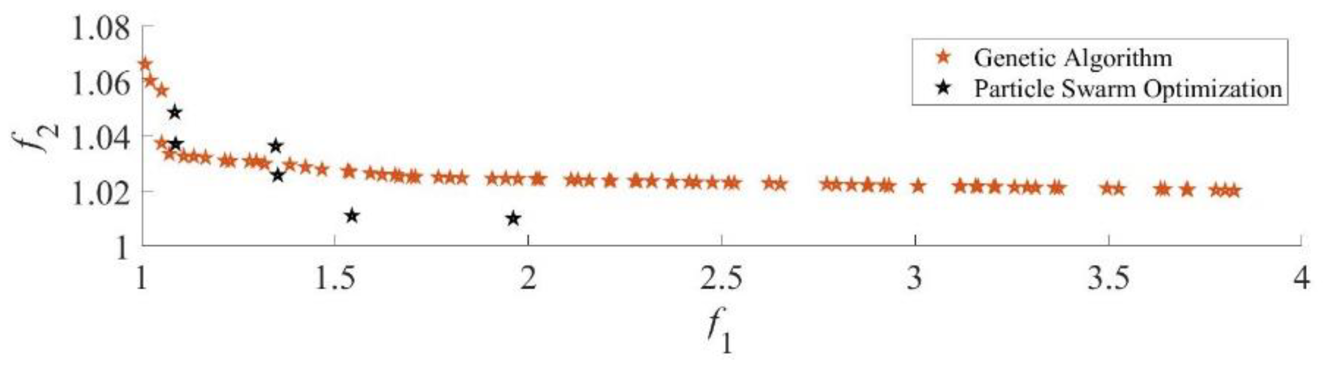
Simplified as double-objective function

$\mathrm{Min}{L}_T$, $\min C$, $\min \delta$, and max$L_h$ were combined into $f_1$; and $\min F$ and $\min M$ were combined into $f_2$. The results of the genetic algorithm and particle swarm optimization are shown in Figure 9.

(2)

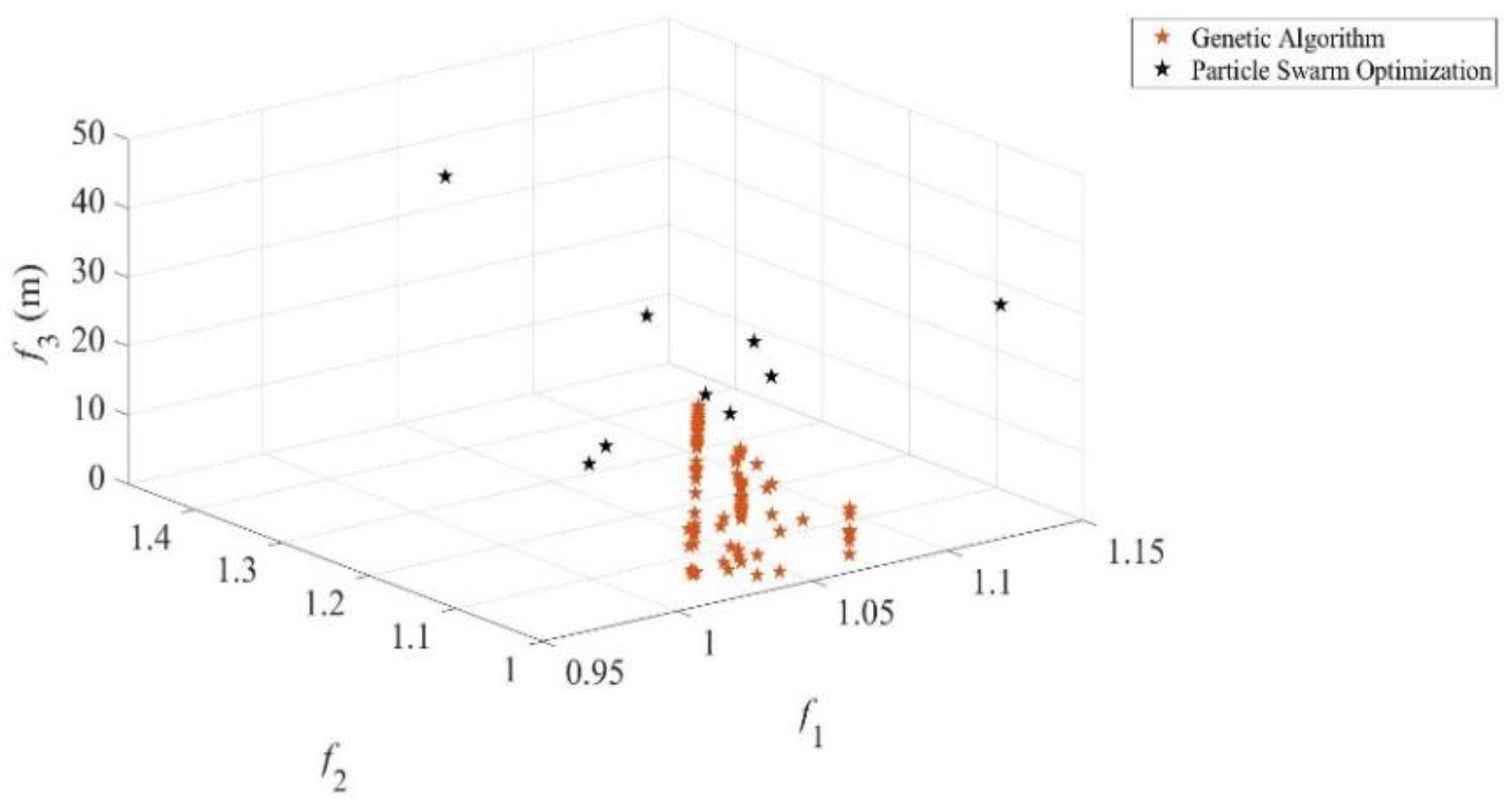
Simplifies to three objective functions

$\mathrm{Min}{L}_T$, $\min C$, and max$L_h$ were combined into $f_1$; $\min F$ and $\min M$ were combined into $f_2$; and $\min \delta$ was $f_3$. The results of the genetic algorithm and particle swarm optimization are shown in Figure 10.

(3)

Simplifies to four objective functions

$\mathrm{Min}{L}_T$ and $\min C$ were merged into $f_1$, $\min F$ and $\min M$ were merged into $f_2$, $\min \delta$ was $f_4$, and $\mathrm{Max}{L}_h$ was $f_4$. The results of the genetic algorithm are shown in Figure 11.

4.3. Comparison of Results

Each objective function’s single objective optimization results are calculated, and a group of multi-objective optimization results are selected. Compared with the original well track design, an overall well track map was drawn, as shown in Figure 12. In the figure, the single objective function optimization results of the smallest wellbore orbit length, the single objective function optimization results of the minimum target error in the first target, and the single objective function optimization results of the minimum drilling cost have small open-hole extension capability in the horizontal section. In contrast, multi-objective function optimization results have better open-hole extension capability in the horizontal section.

Local well track map is shown in Figure 13. In the figure, there is a large error of the target in the original well track. However, the distance error between other optimization results and the second target is relatively small due to the constraints of the second target. The target error of multi-objective function optimization results is relatively small, and the distance error between the first and second targets is within a reasonable range.

The comparison between the original well trajectory design and the multi-objective function optimized well trajectory in the well trajectory length and drilling cost is shown in Figure 14. It can be seen from the figure that with the same drilling time, the multi-objective function optimized well trajectory has obvious advantages; and the distance from the optimized well trajectory to the same target is shorter than that from the original well trajectory. Therefore, it can be proved that the method of multi-objective function optimization of well trajectory is effective.

The comparison between the original well trajectory design and the multi-objective function optimized well trajectory in terms of friction and torque is shown in Figure 15. It can be seen from the figure that the multi-objective function optimized well trajectory is smaller than the original well trajectory design in terms of friction and torque, which can clearly show that the multi-objective function optimized well trajectory is superior to the original well trajectory.

5. Conclusions and Future Works

(1)

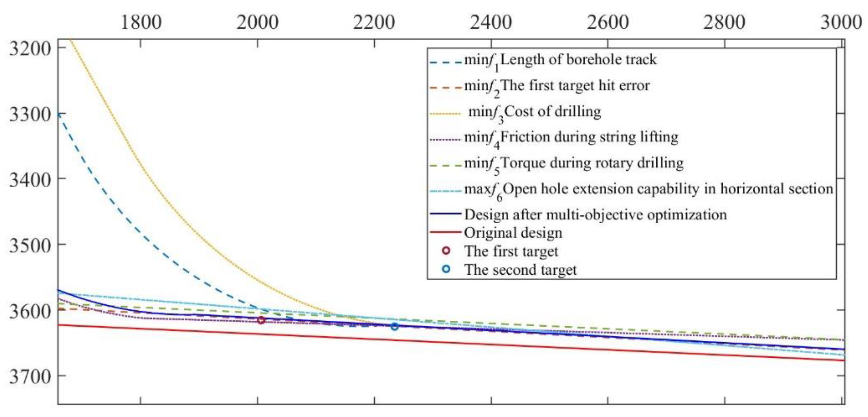
For the three-segment, five-segment, and double-profile extended reach wells, taking into account the formation wellbore stability, formation strength, and deflection tool work to determine the well deflection angle, deflection point location, and target hitting range and other constraints; the optimization objective function of the shortest total length of the borehole; the smallest error of the second target hitting; the lowest cost; and the smallest friction resistance of the pipe string, the smallest rotary drilling torque is established, and the objective function of the longest open-hole extension limit in the horizontal section is established for extended reach wells.

(2)

Taking the extended section well as an example, two objective functions are used to solve the nondominated solution, whose results verify that the friction objective functions of lifting and lowering strings are highly correlated, and one of the minimum friction conditions is taken as the objective function.

(3)

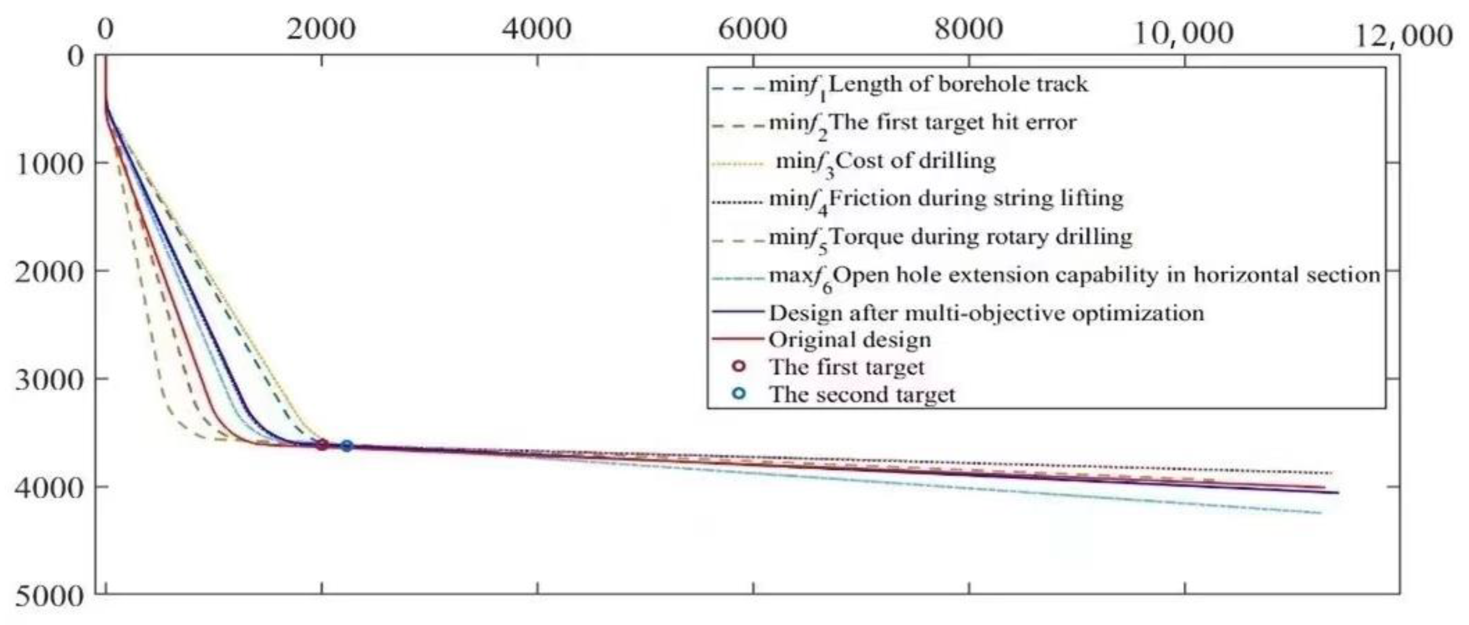
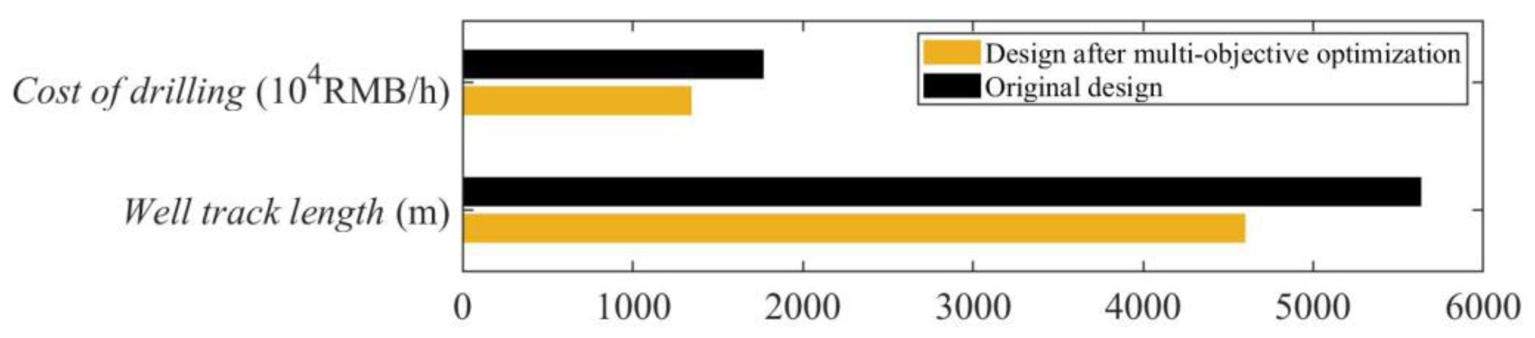
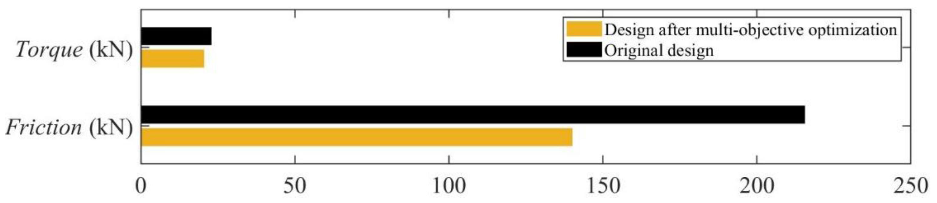
Taking the optimization model of dual profile extended reach well in block 14-8 of the Lufeng Oilfield in the east of the South China Sea as an example and comparing it with the original well trajectory, the well trajectory optimized by multi-objective function can avoid the shortcomings of large target error and poor expansion ability; reduce the track length, friction, and torque; reduce the drilling cost; and achieve the goal of cost reduction and efficiency increase. It is proved that the multi-objective function optimization is practical in application and can provide a certain reference value for the design of well trajectory in field application.

(4)

In the optimization design of well trajectory, in order to reduce costs and more effectively improve productivity, it is also necessary to establish an optimization model based on the three-dimensional trajectory model, optimize the well trajectory by considering more factors, and optimize the well trajectory by using more advanced and richer computer systems and optimization procedures so that the optimization design of well trajectory is closer to reality.

References

1. Chen, X.; Yang, J.; Gao, D.; Hong, Y.; Zou, Y.; Du, X. Unlocking the deepwater natural gas hydrate’s commercial potential with extended reach wells from shallow water: Review and an innovative method. Renew. Sustain. Energy Rev. 2020, 134, 110388. [Google Scholar] [CrossRef]
2. Chen, X.; Du, X.; Yang, J.; Gao, D.; Zou, Y.; He, Q. Developing offshore natural gas hydrate from existing oil & gas platform based on a novel multilateral wells system: Depressurization combined with thermal flooding by utilizing geothermal heat from existing oil & gas wellbore. Energy 2022, 258, 124870. [Google Scholar]
3. Biswas, K.; Vasant, P.M.; Vintaned, J.A.G.; Watada, J. Cellular automata-based multi-objective hybrid Grey Wolf Optimization and particle swarm optimization algorithm for wellbore trajectory optimization. J. Nat. Gas Sci. Eng. 2021, 85, 103695. [Google Scholar] [CrossRef]
4. Abdollahzadeh, B.; Gharehchopogh, F.S. A multi-objective optimization algorithm for feature selection problems. Eng. Comput. 2022, 38, 1845–1863. [Google Scholar] [CrossRef]
5. Akyol, S.; Altas, B. Plant intelligence based metaheuristic optimization algorithms. Artif. Intell. Rev. 2017, 47, 417–462. [Google Scholar] [CrossRef]
6. Hosseini, F.; Gharehchopogh, F.S.; Masdari, M. A Botnet Detection in IoT Using a Hybrid Multi-objective Optimization Algorithm. N. Gener. Comput. 2022, 40, 809–843. [Google Scholar] [CrossRef]
7. Helmy, M.W.; Khalaf, F.; Darwish, T.A. Well design using a computer model. SPE Drill. Complet. 1998, 13, 42–46. [Google Scholar] [CrossRef]
8. Shengzong, J.; Xilu, W.; Limin, C.; Kunfang, L. A new method for designing 3D trajectory in sidetracking horizontal wells under multi-constraints. In SPE Asia Pacific Improved Oil Recovery Conference; OnePetro: Richardson, TX, USA, 1999. [Google Scholar]
9. Zhang, Y.; Wu, S.; Liu, K.; Cao, L.; Yu, L. Research on optimization design method of directional well trajectory. Pet. Drill. Tech. 1999, 27, 3. [Google Scholar]
10. Sui, M.; Zhang, D.; Cheng, W. Optimization design of well trace curve in horizontal Wells. J. Jianghan Pet. Inst. 2000, 22, 25–26. [Google Scholar]
11. Liu, N. Optimization design method of directional well trajectory. J. Jianghan Pet. Inst. 2001, 29, 3. [Google Scholar]
12. Yu, G.; Xing, Y.; Lu, G. Optimization calculation method of trajectory design for oil drilling. J. Shenyang Inst. Aeronaut. Technol. 2003, 20, 3. [Google Scholar]
13. Liu, H.; Meng, Y. Study on optimal trajectory of directional well. T’ien Jan Ch’i K. Yeh 2004, 24, 4. [Google Scholar]
14. Shokir, E.E.M.; Emera, M.K.; Eid, S.M.; Wally, A.W. A new optimization model for 3D well design. Oil Gas Sci. Technol. 2004, 59, 255–266. [Google Scholar] [CrossRef] [Green Version]
15. Lu, G.; Tong, C.; Xing, Y. Three-dimensional multi-target well trajectory design model based on constraint optimization method. Acta Pet. 2005, 26, 3. [Google Scholar]
16. Yan, T.; Liu, W.; Bi, X.; Bi, C. Trajectory optimization design of stepped horizontal Wells. Pet. Drill. Tech. 2007, 29, 3. [Google Scholar]
17. Sun, T. Integrated Method of Horizontal Well Drilling Trajectory Design and Control. Master’s Thesis, China University of Petroleum (Beijing), Beijing, China, 2013. [Google Scholar]
18. Jia, J.; Han, L.; Dou, Y.; Yan, Z.; Huang, G.; Ma, Q. Extended reach well trajectory design method based on multi-objective optimization. J. Guangxi Univ. Nat. Sci. Ed. 2014, 39, 7. [Google Scholar]
19. Atashnezhad, A.; Wood, D.A.; Fereidounpour, A.; Khosravanian, R. Designing and optimizing deviated wellbore trajectories using novel particle swarm algorithms. J. Nat. Gas Sci. Eng. 2014, 21, 1184–1204. [Google Scholar] [CrossRef]
20. Mansouri, V.; Khosravanian, R.; Wood, D.A.; Aadnoy, B.S. 3-D well path design using a multi objective genetic algorithm. J. Nat. Gas Sci. Eng. 2015, 27, 219–235. [Google Scholar] [CrossRef]
21. Wang, Z.; Gao, D.; Yang, J. Design and calculation of complex directional-well trajectories on the basis of the minimum-curvature method. SPE Drill. Complet. 2019, 34, 173–188. [Google Scholar] [CrossRef]
22. Wood, D.A. Hybrid bat flight optimization algorithm applied to complex wellbore trajectories highlights the relative contributions of metaheuristic components. Nat. Gas Sci. Eng. 2016, 32, 211–221. [Google Scholar] [CrossRef]
23. Wang, Z.; Gao, D.; Liu, J. Multi-objective sidetracking horizontal well trajectory optimization in cluster wells based on DS algorithm. J. Pet. Sci. Eng. 2016, 147, 771–778. [Google Scholar] [CrossRef]
24. Sha, L.; Pan, Z. FSQGA based 3D complexity wellbore trajectory optimization. Ind. Eng. Chem. Res. 2018, 73, 79. [Google Scholar] [CrossRef]
25. Huang, W.; Wu, M.; Chen, L. Multi-Objective Drilling Trajectory Optimization with a Modified Complexity Index. In Proceedings of the 37th Chinese Control Conference (CCC), Wuhan, China, 25–27 July 2018. [Google Scholar]
26. Khosravanian, R.; Mansouri, V.; Wood, D.A.; Alipour, M.R. A comparative study of several metaheuristic algorithms for optimizing complex 3-D well-path designs. J. Pet. Explor. Prod. Technol. 2018, 8, 1487–1503. [Google Scholar] [CrossRef] [Green Version]
27. Li, W. Multi-Objective Optimization Technology for Complex Borehole Trajectory. Master’s Thesis, Xi’an Shiyou University, Xi’an, China, 2019. [Google Scholar]
28. Zheng, J.; Lu, C.; Gao, L. Multi-objective cellular particle swarm optimization for wellbore trajectory design. Appl. Soft Comput. 2019, 77, 106–117. [Google Scholar] [CrossRef]
29. Wang, L.; Wei, L.; Gao, Y.; Zhang, Y.; Chen, L.; Zhang, M. Research on 3d horizontal well trajectory optimization design based on multi-objective constraints. Drill. Prod. Technol. 2020, 1, 17–20. [Google Scholar]
30. Khodadadi, N.; Soleimanian Gharehchopogh, F.; Mirjalili, S. MOAVOA: A new multi-objective artificial vultures optimization algorithm. Neural. Comput. Appl. 2022, 1–39. [Google Scholar] [CrossRef]
31. Gharehchopogh, F.S. An Improved Tunicate Swarm Algorithm with Best-random Mutation Strategy for Global Optimization Problems. J. Bionic Eng. 2022, 19, 1177–1202. [Google Scholar] [CrossRef]
32. Liu, X. Research on catenary Track Design Method. T’ien Jan Ch’i K. Yeh 2007, 7, 73–75. [Google Scholar]
33. Liu, X.; Zhou, D.; Li, S.; Gu, L. Design principle and method of parabolic directional well profile. J. Northeast Pet. Univ. 1989, 4, 29–37. [Google Scholar]
34. Wiśniowski, R.; Łopata, P.; Orłowicz, G. Numerical Methods for Optimization of the Horizontal Directional Drilling (HDD) Well Path Trajectory. Energies 2020, 13, 3806. [Google Scholar] [CrossRef]
35. Liu, X. Borehole Trajectory Geometry; Petroleum Industry Press: Beijing, China, 2006. [Google Scholar]
36. Gao, D. Pipe String Mechanics and Engineering in Oil and Gas Wells; China University of Petroleum Press: Beijing, China, 2016. [Google Scholar]
37. Li, X.; Gao, D.; Zhou, Y.; Zhang, H.; Yang, Y. Study on the prediction model of the open-hole extended-reach limit in horizontal drilling considering the effects of cuttings. J. Nat. Gas Sci. Eng. 2017, 40, 159–167. [Google Scholar] [CrossRef]
38. Li, X.; Gao, D.; Zhou, Y.; Cao, W. General approach for the calculation and optimal control of the extended-reach limit in horizontal drilling based on the mud weight window. J. Nat. Gas Sci. Eng. 2016, 35, 964–979. [Google Scholar] [CrossRef]
39. Li, X.; Gao, D.; Zhou, Y.; Zhang, H. A model for extended-reach limit analysis in offshore horizontal drilling based on formation fracture pressure. J. Pet. Sci. Eng. 2016, 146, 400–408. [Google Scholar] [CrossRef]
40. Holt, F.; Lane, H.; Lisnas. Rock Mechanics in Petroleum Engineering: English-Chinese Reference; Petroleum Industry Press: Beijing, China, 2010. [Google Scholar]
41. Chen, J.; Liu, Z. Drilling Engineering Design Method for Deepwater Exploration Wells; Petroleum Industry Press: Beijing, China, 2014. [Google Scholar]
42. Runar, N.; Robin, H. Steering Response for Directional Well in Soft Formation in Deep Water Development; Offshore Technology Conference: Houston, TX, USA, 2008. [Google Scholar]
43. Zheng, D.; Zhang, H.; Zhu, Y.; Sun, W. Influence mechanism of rock mechanical properties on well trajectory. Pet. Drill. Tech. 2014, 42, 5. [Google Scholar]
44. Zhao, W. Research and Application of Drilling Technology in the Tuo Putai Block of Tahe Oilfield. Master’s Thesis, China University of Petroleum (east China), Qingdao, China, 2018. [Google Scholar]
45. Meng, Q. Optimization of Horizontal Well Trajectory in Dibeilla Block, Niger. Master’s Thesis, China University of Petroleum (Beijing), Beijing, China, 2020. [Google Scholar]
Figure 1. Arc line model of build-up section.
Applsci 12 10722 g001
Figure 2. Force analysis of hold section. (a) Lifting process; (b) lowering process.
Applsci 12 10722 g002
Figure 3. Force analysis of build-up section unit string. (a) Lifting process; (b) lowering process.
Applsci 12 10722 g003
Figure 4. Force analysis of build-off section unit string. (a) Lifting process; (b) lowering process.
Applsci 12 10722 g004
Figure 5. Three-section wellbore trajectory profile.
Applsci 12 10722 g005
Figure 6. Five-section wellbore trajectory profile.
Applsci 12 10722 g006
Figure 7. Two build-up trajectory profile.
Applsci 12 10722 g007
Figure 8. Pareto of pairwise objective functions.
Applsci 12 10722 g008
Figure 9. Pareto of bi-objective function.
Applsci 12 10722 g009
Figure 10. Pareto of tri-objective function.
Applsci 12 10722 g010
Figure 11. Pareto of four-objective function.
Applsci 12 10722 g011
Figure 12. Overall borehole trajectory.
Applsci 12 10722 g012
Figure 13. Part of borehole trajectory.
Applsci 12 10722 g013
Figure 14. Comparison of track length and drilling costs.
Applsci 12 10722 g014
Figure 15. Comparison of friction and torque.
Applsci 12 10722 g015