Abstract
Structural network pruning is an effective way to reduce network size for deploying deep networks to resource-constrained devices. Existing methods mainly employ knowledge distillation from the last layer of network to guide pruning of the whole network, and informative features from intermediate layers are not yet fully exploited to improve pruning efficiency and accuracy. In this paper, we propose a block-wisely supervised network pruning (BNP) approach to find the optimal subnet from a baseline network based on knowledge distillation and Markov Chain Monte Carlo. To achieve this, the baseline network is divided into small blocks, and block shrinkage can be independently applied to each block under a same manner. Specifically, block-wise representations of the baseline network are exploited to supervise subnet search by encouraging each block of student network to imitate the behavior of the corresponding baseline block. A score metric measuring block accuracy and efficiency is assigned to each block, and block search is conducted under a Markov Chain Monte Carlo scheme to sample blocks from the posterior. Knowledge distillation enables effective feature representations of the student network, and Markov Chain Monte Carlo provides a sampling scheme to find the optimal solution. Extensive evaluations on multiple network architectures and datasets show BNP outperforms the state of the art. For instance, with 0.16% accuracy improvement on the CIFAR-10 dataset, it yields a more compact subnet of ResNet-110 than other methods by reducing 61.24% FLOPs.
1. Introduction
As a long-standing research interest in the computer vision domain, neural network pruning aims to compress a large deep neural network (DNN) without significant degradation of model performance, such that it can be deployed on resource-constrained devices. Specifically, structured pruning [1] aims to obtain a reduced architecture (subnet) of a baseline network; it examines regular structures of the network to remove redundant filters and neurons and has shown remarkable advantages in improving the computational efficiency of DNNs.
An arsenal of methods for structured network pruning has been developed in recent years. A majority of these methods follow a conventional way of network pruning that involves two iterative steps, i.e., subnet search and evaluation. During the search step, a subnet is selected from all feasible proposals for evaluation, while in the evaluation step, the performance of the selected subnet is assessed on a validation set. For instance, autoML for model compression (AMC) [2] leveraged reinforcement learning to yield subnets in a layer-wise manner. Gan et al. [3] proposed a two-stage approach to streamline the network to better balance accuracy and speed. However, these methods suffer from limited scalability since evaluations of a large number of subnets on a full validation set are required to find the optimal subnet. To avoid an extensive search for candidate subnets, Liebenwein et al. [4] proposed to yield subnets through sampling each filter with the probability proportional to the importance score of the filter. Recently, learned global ranking (LeGR) [5] inferred a global ranking of the filters via layer-wise affine transformations for generating subnets that meet different tradeoffs between model accuracy and latency. However, most of these methods rely on local information or adopt hard thresholds to remove filters, which may result in suboptimal solutions. In addition, informative features from intermediate layers of the network may be helpful to elevate the performance of network pruning and are not fully exploited in the existing methods.
There are some methods to learn sparse structures of networks under a differentiable or an end-to-end manner. These methods often use learnable masks to implicitly prune unimportant filters. For example, Lin et al. [6] used a soft mask to scale output of each structure and removed structures with a zero mask under a generative adversarial framework. Similarly, You et al. [7] attached channel-wise scaling factors to original networks for differentiable filter pruning. These methods usually need to find a hard threshold to remove the filters with near-zero masks, which may heavily damage the performance of networks [6]. Moreover, the training of architecture-related hyperparameters often suffers from low stability.
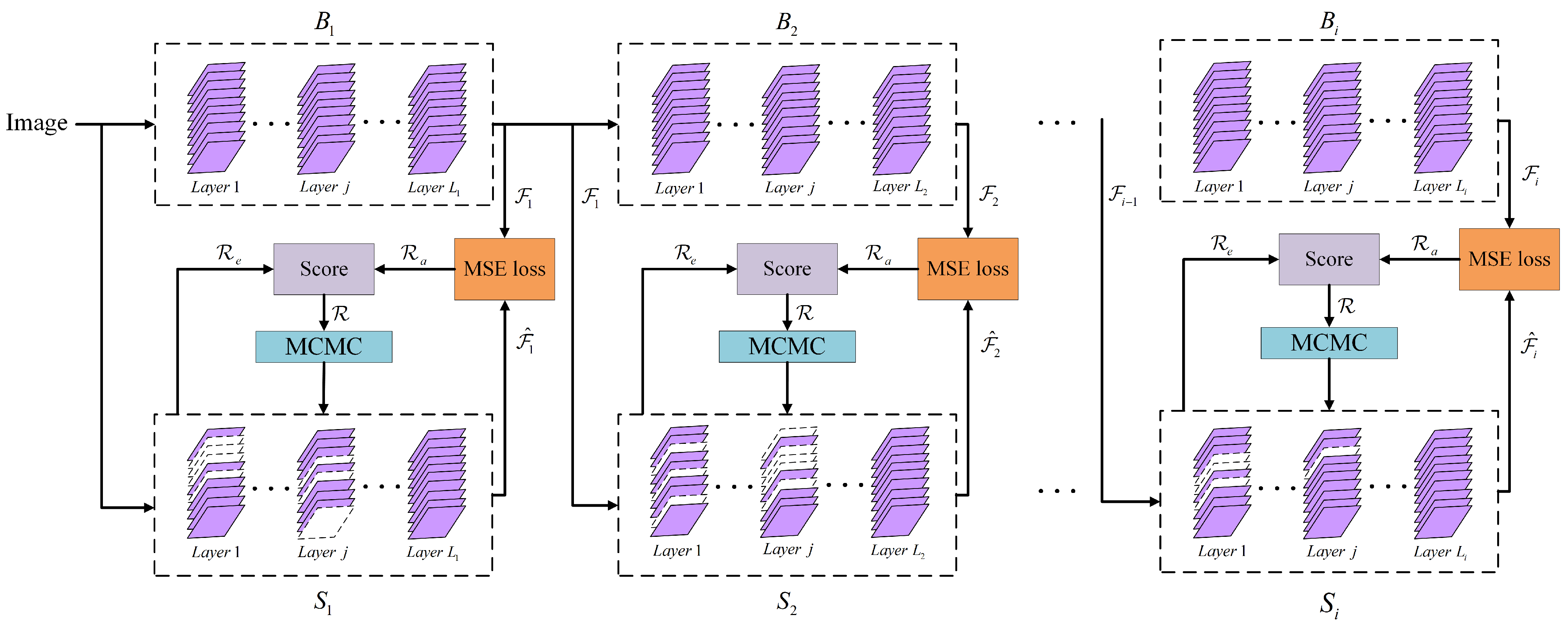
To achieve a good trade-off between efficiency and accuracy for subnet search, we introduce a novel block-wisely supervised network pruning (BNP) method based on knowledge distillation (KD) [8] and Markov Chain Monte Carlo (MCMC) [9]. Our work is inspired by the recent success of Neural Architecture Search (NAS) in supernet training under a block-wise manner [10]. As shown in Figure 1, we first divide the baseline (teacher) network and pruned (student) network into several blocks following the same strategy, then independently prune individual blocks by transferring block-wise knowledge from teacher network to student network. This allows parallelization of block shrinkage among all blocks in an analogous way, and thus improves subnet search efficiency. For each student block, our method samples substructures from the posterior under an MCMC scheme to find the optimal substructure. In addition, a neighborhood-based policy is employed to define the state transitions from the current substructure. Our main contributions are three-fold:
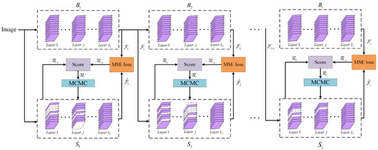
Figure 1.
Illustration of our BNP. Network pruning is decomposed into block-wise shrinkage based on knowledge distillation. The blocks at the top form teacher network, and the blocks at the bottom constitute student network. Each student block is independently compressed to imitate the behavior of the corresponding teacher block by minimizing the MSE loss between output feature maps. Markov Chain Monte Carlo is used to sample substructures for evaluation by scoring each substructure with accuracy metric and efficiency metric .
- 1.
- We propose block-wisely supervised network pruning to compress a baseline network by removing semantically similar structures without heavily sacrificing model accuracy.
- 2.
- Based on block-wise KD for learning effective feature representation and an MCMC scheme for sampling subnets from the posterior, BNP is able to find the optimal reduced architecture.
- 3.
- The evaluation results of BNP on multiple network architectures and datasets suggest it has advantages in yielding higher pruning rates and less accuracy drop than state-of-the-art (SOTA) methods.
2. Related Works
2.1. Network Pruning
Network pruning aims to deliver a well-performing lightweight network by eliminating redundant weights or structured units of a baseline network. Based on adopted pruning granularity, network pruning can be divided into structured [11,12] and unstructured pruning [13]. Unstructured network pruning, also called weight pruning, achieves a sparse weight matrix by removing unimportant weight parameters. For instance, Han et al. [13] introduced a threshold-based pruning algorithm to remove weights with absolute values below a threshold. Unstructured pruning leads to irregular weight tensors and requires appropriate software and hardware to achieve acceleration. By comparison, structured pruning removes the redundant structures of the network such as convolutional kernels, layers, and channels to achieve a true significant acceleration of the network.
Structured pruning can be viewed as two subtasks: allocation of network sparsity [6,14] and selection of important units within layers [15,16]. For each layer of the network, global importance of the network structure and compression ratio determine the distribution of network sparsity under the limited resources. For example, Ashok et al. [14] introduced a two-stage pruning algorithm that first finds redundant layers and then reasons unimportant convolutional kernels within the layers via reinforcement learning. Lin et al. [6] used soft masks to find compression rates of blocks, branches, and channels in a network. The selection of important structures within layers is performed by ranking the importance of convolutional kernels and neurons for each layer. For instance, Lin et al. [15] calculated the rank of feature maps as the importance score of each channel and sorted the channels in each layer based on the ranks to remove less important channels. Ide et al. [16] proposed to remove redundant feature maps by utilizing empirical classification loss.
2.2. Knowledge Distillation
The basic idea of knowledge distillation is to first train a large network (teacher network) and transfer the knowledge learned in the large network to a smaller network (student network) [17,18]. For example, Hinton et al. [17] introduced a compression framework for knowledge distillation that trains the student network with the soft labels of the teacher network. There has been an increasing interest in applying knowledge distillation to network pruning. KD can also be applied to the middle layers of the teacher network where rich representation information can be extracted. Li et al. [19] used knowledge distillation and NAS to design a general-purpose compression scheme that reduces the computation and memory consumption of generators in Conditional Generative Adversarial Networks. Romero et al. [20] proposed a knowledge-distillation-based FitNet to guide training of the student network by exploiting outputs of the teacher network and features of intermediate layers. In this paper, the baseline and pruned networks are treated as teacher and student networks, respectively. We divide both networks into distinct blocks and use block-wise representations of the teacher network to supervise student network pruning by sampling candidate subnets via MCMC.
3. Method
In this section, we provide a detailed presentation of the proposed BNP framework for reasoning reduced architecture from a baseline network. As shown in Figure 1, our method builds on block-wise KD and MCMC schemes that allow effective subnet search and evaluation.
3.1. Block-Wise Network Pruning
As different parts of DNN deliver distinct patterns of an image [10], we divide the baseline network into blocks and perform channel pruning on individual blocks to improve efficiency. Each block contains an arbitrary number of layers, including convolutional and fully connected (FC) layers. Block shrinkage is independently applied to each block to yield a reduced substructure, then all the resulting substructures are connected to constitute the final subnet. Inspired by the recent success of neural architecture search in efficiently training supernets [10], we utilize block-wise representation of the baseline network to supervise subnet search, such that each block can be pruned independently in an analogous manner. As shown in Figure 1, the (i-1)-th block of the teacher network outputs feature map , the i-th block of the student network takes as input and outputs feature map to imitate the block-wise output of the teacher network. To effectively measure the knowledge transferred from the i-th block, we define an accuracy metric based on the MSE loss between and :
where Z is a substructure of the i-th block, denotes input image, represents validation dataset, and n is the number of samples in . Note that our block-wise search does not rely on labels of input data.
To further discriminate between different substructures that show similar accuracy but different computational efficiency, the FLOPs’ reduction rate is employed to define the efficiency metric:
where and denote the FLOPs of the reduced and baseline blocks, respectively. FLOPs of FC layer are calculated as ; here, and are the height and width of the feature map, and and are the numbers of input and output channels. In addition, the FLOPs of the convolutional layer are measured as ; here, and are the height and width of the convolutional kernel.
By taking a tradeoff between and , we derive a metric to score each substructure by considering both model capability and efficiency:
where is introduced to control the weights of two terms. Higher values of will give a preference to substructures that have more significant FLOP reductions. Based on the above definition, for each block of student network we need to find the best-performing substructure that shows the highest value of .
3.2. MCMC-Based Substructure Search
Considering that all blocks can be independently optimized under an analogous manner, we use S to denote a block of the student network and Z to denote a substructure of S without loss of generality. Let L be the number of layers in block S and be the number of filters in the j-th layer of block S; we aim to find the optimal number of filters to be preserved in each layer. This problem can be defined as the following optimization problem:
where represents a substructure, and each element denotes the number of preserved filters or neurons in the j-th layer, defines all candidate substructures of the block S, and is the performance metric defined in Equation (3) to evaluate the goodness of the substructure Z.
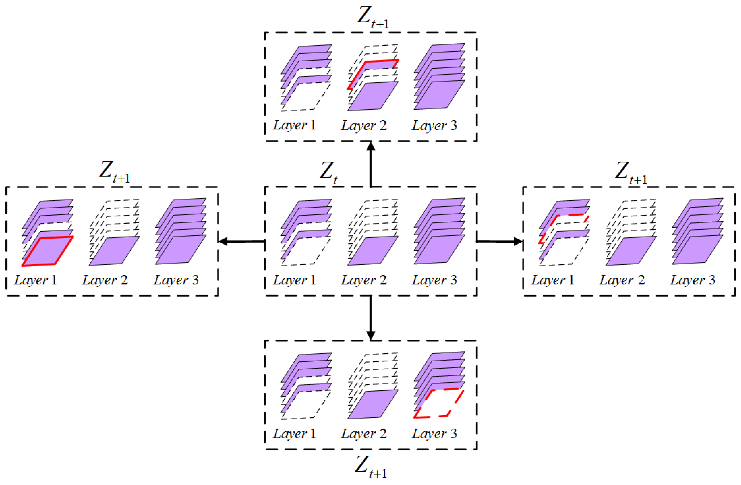
We select the preserved filters by ranking the filters with importance scores; therefore, there are candidate substructures that may constitute a large search space, suggesting an exhaustive search is impractical. Instead, with Equation (3), we sample substructures from the posterior under an MCMC scheme to find the maximum likelihood estimation (MLE) of the substructure. Formally, from the current state , a new state is proposed based on transition probability . We sample a move from all feasible moves from to obtain the next state . The feasible moves are defined by the following criteria:
where denotes -norm, and is an integer number to bound the moves within a small space. Figure 2 illustrates the feasible moves under . The proposals constrained by the above condition are called the neighborhoods of . The move from to is accepted with probability:
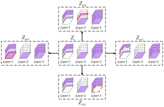
Figure 2.
Illustration of feasible transitions from current state to next state under . The added or deleted channel is marked by red border.
To find the optimal solution, we initialize to meet a desired FLOPs’ reduction rate and restart the MCMC chain multiple times. The maximally performing substructure during search is selected as the best solution. Each block of the baseline network is pruned by following the same procedure. A brief description of the MCMC scheme is provided in Algorithm 1.
| Algorithm 1: MCMC scheme in BNP. |
Input: A student block S, input data X in validation dataset, number of restarts N, length of each MCMC repetition M. Output: Reduced substructure.
|
3.3. Filter Selection for Each Layer
We define the importance of a filter as the -norm of its kernel weights [21] and generate a priority ordering of the filters, i.e., descending order based on the importance scores for each layer of the network. For the j-th layer of a given block S, we select top-ranked filters to build the layer of Z, and the weights of the replicated filters are not fine-tuned for fast evaluation. This can to some extent compensate for the low efficiency of MCMC sampling and provide a reasonable balance between model accuracy and efficiency.
4. Experiments
The evaluations were conducted on two network models, i.e., VGG Very Deep Convolutional Networks (VGGNet) and Residual Neural Networks (ResNet), using three datasets including CIFAR-10, CIFAR-100 [22], and ImageNet Large-Scale Visual Recognition Challenge (ILSVRC-2012) [23]. The VGG-16 architecture adopted in [21] was used as the VGGNet model [24], ResNet-20, ResNet-50, ResNet-56, and ResNet-110 were used as the ResNet models [25]. CIFAR-10 consists of 32 × 32 natural images from 10 classes. CIFAR-100 is similar to CIFAR-10 but contains 100 classes. Both CIFAR-10 and CIFAR-100 datasets consist of 60,000 images, and the original training set was divided into a training set with a size of 45,000 and a validation set with a size of 5000. ImageNet contains a 1000-category color image dataset consisting of 1.2 million training images and 50,000 validation images.
The training dataset was used to train the baseline network and fine-tune the pruned network; the validation dataset was used to quickly assess the performance of subnets, and the test dataset was employed to evaluate the performance of the finally obtained pruned network. The training, validation, and test datasets were determined at the very beginning and kept fixed across different tests. For assessing pruning performance, we use accuracy drop as the performance metric to compare different methods.
4.1. Implementation Details
The parameters used to train networks are as follows: For CIFAR dataset, the baseline networks were trained for 300 epochs using the stochastic gradient descent (SGD) algorithm; the learning rate was initialized to 0.1 and decremented by a factor of 10 at 120, 180, and 240 epochs; and batch size, momentum, and weight decay were set to 256, 0.9, and , respectively. During subnet search, the subnet was not fine-tuned for fast evaluation on the validation set. At the end of network pruning, we initialized the learning rate to 0.01 and set other parameters to the same values as in the baseline network to fine-tune the pruned network. For ImageNet, we used ResNet-50 to evaluate the performance; the baseline network was trained for 50 epochs using the SGD algorithm; the learning rate was initialized to 0.1 and adjusted using the cosine descent method; and batch size, momentum, and weight decay were set to 256, 0.9, and , respectively. During the training process, data enhancement methods such as random cropping, random PCA noise, and random flipping were employed. In the validation set, we performed a random center crop of the images by first enlarging the image to a size of 256 and then cropping a -sized region in the center of the image. We conducted all experiments using a single NVIDIA TITAN V GPU on a machine with 128 GB RAM and implemented our method with the TensorFlow framework.
The baseline network was divided into several blocks. The VGGNet consists of convolutional layers and fully connected layers. ResNet is composed of multiple residual blocks, each of which includes multiple convolutional layers and a shortcut connection. For VGG-16, we directly searched a subnet by treating the whole baseline network as a block. Every 3 residual blocks for ResNet-20 constitute a block S to prune. For ResNet-56 and ResNet-110, we treated every 9 residual blocks as a block S to prune. ResNet-50 consists of 5 stages, where the 1st stage is a single convolutional layer and the remaining 4 stages consist of 3, 4, 6, and 3 bottlenecks, respectively. In the pruning process, the 1st stage was not pruned, and each of the remaining 4 stages was used as a block to prune. For MCMC sampling, we set the number of restarts, burn-in periods, thinness, and length of each MCMC chain to 10, 3000, 1, and 6000, respectively, and randomly initialized the state of each restart to meet a FLOPs’ reduction of ∼50%. The pruning results with hyperparameter and were analyzed.
4.2. Results
4.2.1. Results on CIFAR-10
VGGNet: We first evaluated the performance of BNP in compressing VGGNet, and the results are depicted in Table 1. Our method prunes 54% of FLOPs with a cost of 0.37% accuracy drop under . The high rank of the feature maps (HRank) [15] reaches a similar FLOP reduction rate but sacrifices the accuracy by 0.53%. Generative adversarial learning (GAL) [6] can prune 45.2% of FLOPs with a cost of similar accuracy loss of 0.54%. Sparse structure selection (SSS) [26] is able to reduce 41.6% of FLOPs but results in a much-degraded model performance with 0.94% accuracy loss. Note that our method presents lower rates in pruning parameters than the competitors, which is attributed to the fact that BNP takes FLOP reduction as the objective, as shown in Equation (2). One can expect an elevated pruning rate of parameters by reformulating the efficiency score with the pruning rate of parameters.

Table 1.
Network pruning results of VGGNet on CIFAR-10. In all tables, Paras↓ denotes parameters reduction, FLOPs↓ represents FLOPs reduction, and Acc↓ means accuracy loss on test dataset.
ResNet-56: We further examined the effectiveness of BNP in compressing the residual network ResNet-56. The performance of our method was compared with that of the state-of-the-art methods, and the results are shown in Table 2. With , BNP performs much better than the RL-based method AMC [2] in reducing FLOPs (62.97% vs. 50%), as well as preserving model accuracy (0.16% vs. 0.9% accuracy loss). With a similar FLOP pruning rate, our method shows significantly better performance in preserving model capability than the adversarial learning-based method GAL (0.16% vs. 1.68% accuracy loss). In addition, our method also outperforms filter pruning via geometric median (FPGM) [27], learning filter pruning criteria (LFPC) [28], differentiable sparsity allocation (DSA) [29], and dynamic and progressive filter pruning (DPFPS) [30] by yielding more compact substructures and sacrificing less model accuracy. With , BNP produces a compact subnet with 66.29% of FLOPs reduced and 0.66% accuracy drop. These results imply our method is effective in learning block-wise knowledge from baseline networks, and thus has advantages in delivering better substructures than the competitors.
Table 2.
Network pruning results of ResNet-56 on CIFAR-10.
ResNet-110: We proceed to assess BNP in a much deeper neural network ResNet-110, and the comparison results between different methods are depicted in Table 3. Our method achieves consistently better pruning results than the SOTA methods. For instance, BNP improves model accuracy by 0.16% after removing 59.9% parameters and 61.24% FLOPs, while HRank [15] results in 0.14% accuracy loss under a similar pruning rate of parameters and FLOPs (59.2% and 58.2%). LFPC is also effective in improving model efficiency and capability with 60.3% FLOP removal and 0.11% increased accuracy. By delivering the same model capability, BNP removes more FLOPs than FPGM [27] (61.24% vs. 52.3%). In addition, our method can remove as high as 67.86% of parameters and 61.44% of FLOPs without attenuating model accuracy. Increasing the hyperparameter to 0.2 results in a more compact network by removing 69.21% of FLOPs without heavy damage to model accuracy. The enhanced ability of BNP builds on the effective feature representations via block-wise KD.
Table 3.
Network pruning results of ResNet-110 on CIFAR-10.
4.2.2. Results on CIFAR-100
To assess the capability of BNP on complex vision classification tasks, we applied BNP to the pruning of Resnet-56 on CIFAR-100. The results indicate our method has similarly good performance in removing redundant structures. As shown in Table 4, BNP reaches better results in both reducing FLOPs and preserving accuracy of the baseline network than other methods when . With a cost of 0.55% accuracy loss, it produces a compact subnet by removing 58.08% of parameters and 53.78% of FLOPs, while other methods result in as high as 2.61% accuracy degradation under similar pruning level. Our method also yields a more efficient subnet by reduction of 61.34% of FLOPs and sacrificing less than 1% accuracy. These results suggest the proposed method is also practically effective in network compression on complex tasks.
Table 4.
Network pruning results of ResNet-56 on CIFAR-100.
4.2.3. Results on ImageNet
To further examine the effectiveness of BNP in pruning networks on large datasets, we applied it to ResNet-50 on ImageNet dataset. The performance comparison results of the SOTA methods are shown in Table 5. It is observed that our method is able to compress more FLOPs with less model accuracy loss when . For instance, with a FLOP reduction rate of 51%, BNP shows similar Top-5 accuracy loss as that of the autopruner (AP) [32] (0.73% vs. 0.72%), while achieving less than Top-1 accuracy loss (1.27% vs. 1.39%). Compared with DSA [29], BNP eliminates more FLOPs as well as better maintains the model capability in both Top-1 and Top-5 accuracy. Our method also trims more FLOPs at less loss of accuracy when compared with channel pruning (CP) [1], FPGM [27], SCP [33], and the artificial bee colony algorithm (ABC) [34]. With the same FLOP reduction of 55%, BNP yields much better results than GAL [6] in maintaining both Top-1 and Top-5 accuracies. In addition, at a higher FLOP reduction rate of 63%, BNP still performs acceptably well in rebuilding the model capability, with only 1.93% of Top-1 and 1.09% of Top-5 accuracy loss, while removing 59.91% of parameters. By comparison, HRank [15] achieves 4.17% of Top-1 and 1.86% of Top-5 loss with 62.10% of FLOPs and 46.00% of parameters reduced. The results suggest BNP is effective in pruning networks even on more complex datasets.
Table 5.
Network pruning results of ResNet-50 on ImageNet. Where Top-1/Top-5 Acc denotes Top-1/Top-5 accuracy, Top-1 Acc↓/Top-5 Acc↓ means accuracy loss.
4.3. Ablation Study
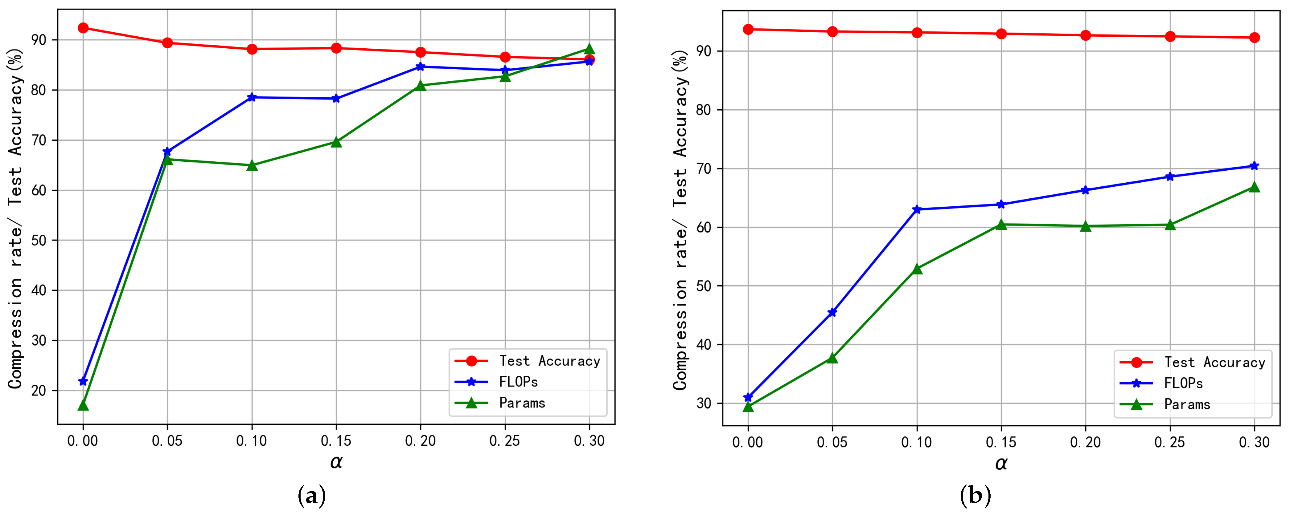
To evaluate the effects of hyperparameter on network pruning, we compared the pruning results of ResNet-20 and ResNet-56 on CIFAR-10 under different values in [0, 0.3] with an increment of 0.05. The pruning process is repeated three times for each value to calculate the median measures. Figure 3 shows the value of has a significant effect on the pruning rates of parameters and FLOPs and model accuracy on testing sets. As expected, the FLOP and parameter reduction rates increase with the , while model accuracy drops with the . For instance, only 17.07% of parameters and 21.82% of FLOPs of ResNet-20 are removed under , and corresponding rates are elevated to 88.22% and 85.64% under . The maximum changes in pruning rates for ResNet-20 are observed when the value of increases from 0 to 0.05, and the results in Table 6 suggest small changes in result in significantly different compression rates of FLOPs. Similar changes with are observed for compression rates and test accuracy of ResNet-56 (as shown in Figure 3b), which indicates BNP generalizes well on different network architectures. These results demonstrate our method is highly adaptive to different memory and computational constraints by setting appropriate values of .

Figure 3.
The effects of hyperparameter on network pruning results. (a) ResNet-20; (b) ResNet-56.
Table 6.
Pruning results of ResNet-20 on CIFAR-10 when hyperparameter is set to 0.01, 0.02 and 0.03.
5. Conclusions
In this paper, we introduce a block-wisely supervised network pruning approach to effectively eliminate structural redundancy of a baseline network. The KD technique is employed to independently mimic block-wise feature representations of baseline networks, and an MCMC scheme is employed to sample substructures from the posterior. Extensive benchmarking tests of BNP in pruning popular neural network architectures on three datasets demonstrate our method has advantages over the SOTA. The limitation of BNP lies in that pruning ResNet networks on ImageNet with MCMC sampling is computationally expensive, and we plan to improve its efficiency by designing more efficient sampling methods.
Author Contributions
Conceptualization, H.L. and Z.Y.; methodology, F.D. and Z.Y.; software, F.D.; validation, H.L., F.D. and Z.Y.; formal analysis, H.L.; data curation, F.D.; investigation, H.L., F.D. and L.S.; project administration, H.L., L.S. and Z.Y.; supervision, Z.Y.; resources, F.D. and L.S.; writing—original draft, H.L. and Z.Y.; visualization, H.L.; writing—review and editing, H.L., F.D. and Z.Y.; funding acquisition, F.D., L.S. and Z.Y. All authors have read and agreed to the published version of the manuscript.
Funding
This work was supported in part by the National Natural Science Foundation of China (61901238, 62062058), the Key Research and Development Program of Ningxia (2019BEB04023, 2021BEE03013), and the West Light Foundation of the Chinese Academy of Sciences (XAB2019AW12).
Institutional Review Board Statement
Not applicable.
Informed Consent Statement
Not applicable.
Data Availability Statement
The ILSVRC-2012, CIFAR-10, and CIFAR-100 datasets used to support the findings of this study are available at https://image-net.org/challenges/LSVRC/2012/ (accessed on 10 August 2022) http://www.cs.toronto.edu/~kriz/cifar-10-python.tar.gz (accessed on 10 August 2022) and http://www.cs.toronto.edu/~kriz/cifar-100-python.tar.gz (accessed on 10 August 2022).
Conflicts of Interest
The authors declare no conflict of interest.
References
- He, Y.; Zhang, X.; Sun, J. Channel pruning for accelerating very deep neural networks. In Proceedings of the International Conference on Computer Vision (ICCV), Venice, Italy, 22–29 October 2017; pp. 1389–1397. [Google Scholar]
- He, Y.; Lin, J.; Liu, Z.; Wang, H.; Li, L.; Han, S. Amc: Automl for model compression and acceleration on mobile devices. In Proceedings of the European Conference on Computer Vision (ECCV), Munich, Germany, 8–14 September 2018; pp. 784–800. [Google Scholar]
- Gan, J.; Wang, W.; Lu, K. Compressing the cnn architecture for in-air handwritten chinese character recognition. Pattern Recognit. Lett. 2020, 129, 190–197. [Google Scholar] [CrossRef]
- Liebenwein, L.; Baykal, C.; Lang, H.; Feldman, D.; Rus, D. Provable filter pruning for efficient neural networks. In Proceedings of the International Conference on Learning Representations (ICLR), Online, 26 April–1 May 2020. [Google Scholar]
- Chin, T.W.; Ding, R.; Zhang, C.; Marculescu, D. Towards efficient model compression via learned global ranking. In Proceedings of the Computer Vision and Pattern Recognition (CVPR), Seattle, WA, USA, 13–19 June 2020. [Google Scholar]
- Lin, S.; Ji, R.; Yan, C.; Zhang, B.; Cao, L.; Ye, Q.; Huang, F.; Doermann, D. Towards optimal structured cnn pruning via generative adversarial learning. In Proceedings of the Computer Vision and Pattern Recognition (CVPR), Long Beach, CA, USA, 16–20 June 2019; pp. 2790–2799. [Google Scholar]
- You, Z.; Yan, K.; Ye, J.; Ma, M.; Wang, P. Gate decorator: Global filter pruning method for accelerating deep convolutional neural networks. In Proceedings of the Advances in Neural Information Processing Systems, Vancouver, BC, Canada, 8–14 December 2019; pp. 2133–2144. [Google Scholar]
- Wang, H.; Zhao, H.; Li, X.; Tan, X. Progressive blockwise knowledge distillation for neural network acceleration. In Proceedings of the International Joint Conference on Artifificial Intelligence (IJCAI), Stockholm, Sweden, 13–19 July 2018; pp. 2769–2775. [Google Scholar]
- Gasparini, M. Markov chain monte carlo in practice. Technometrics 1999, 39, 338. [Google Scholar] [CrossRef]
- Li, C.; Peng, J.; Yuan, L.; Wang, G.; Liang, X.; Lin, L.; Chang, X. Block-wisely supervised neural architecture search with knowledge distillation. In Proceedings of the Computer Vision and Pattern Recognition (CVPR), Seattle, WA, USA, 13–19 June 2020. [Google Scholar]
- Wang, Z.; Li, C.; Wang, X. Convolutional neural network pruning with structural redundancy reduction. In Proceedings of the Computer Vision and Pattern Recognition (CVPR), Online, 19–25 June 2021; pp. 14913–14922. [Google Scholar]
- Osaku, D.; Gomes, J.; Falcão, A. Convolutional neural network simplification with progressive retraining. Pattern Recognit. Lett. 2021, 150, 235–241. [Google Scholar]
- Han, S.; Pool, J.; Tran, J.; Dally, W. Learning both weights and connections for efficient neural network. In Proceedings of the Advances in Neural Information Processing Systems, Montreal, PC, Canada, 7–12 December 2015; pp. 1135–1143. [Google Scholar]
- Ashok, A.; Rhinehart, N.; Beainy, F.; Kitani, K.M. N2n learning: Network to network compression via policy gradient reinforcement learning. In Proceedings of the International Conference on Learning Representations (ICLR), Vancouver, BC, Canada, 30 April–3 May 2018. [Google Scholar]
- Lin, M.; Ji, R.; Wang, Y.; Zhang, Y.; Zhang, B.; Tian, Y.; Shao, L. Hrank: Filter pruning using high-rank feature map. In Proceedings of the Computer Vision and Pattern Recognition (CVPR), Seattle, WA, USA, 13–19 June 2020; pp. 1526–1535. [Google Scholar]
- Ide, H.; Kobayashi, T.; Watanabe, K.; Kurita, T. Robust pruning for efficient cnns. Pattern Recognit. Lett. 2020, 135, 90–98. [Google Scholar] [CrossRef]
- Hinton, G.; Vinyals, O.; Dean, J. Distilling the knowledge in a neural network. arXiv 2015, arXiv:1503.02531. [Google Scholar]
- Zaras, A.; Passalis, N.; Tefas, A. Improving knowledge distillation using unified ensembles of specialized teachers. Pattern Recognit. Lett. 2021, 146, 215–221. [Google Scholar] [CrossRef]
- Li, M.; Lin, J.; Ding, Y.; Liu, Z.; Zhu, J.-Y.; Han, S. Gan compression: Efficient architectures for interactive conditional gans. In Proceedings of the Computer Vision and Pattern Recognition (CVPR), Seattle, WA, USA, 13–19 June 2020; pp. 5284–5294. [Google Scholar]
- Romero, A.; Ballas, N.; Kahou, S.E.; Chassang, A.; Gatta, C.; Bengio, Y. Fitnets: Hints for thin deep nets. In Proceedings of the International Conference on Learning Representations (ICLR), San Diego, CA, USA, 7–9 May 2015. [Google Scholar]
- Li, H.; Kadav, A.; Durdanovic, I.; Samet, H.; Graf, H.P. Pruning filters for efficient convnets. In Proceedings of the Advances in Neural Information Processing Systems (NIPS 2017), Long Beach, CA, USA, 4–7 December 2017. [Google Scholar]
- Krizhevsky, A.; Hinton, G. Learning Multiple Layers of Features from Tiny Images; Technical Report; Citeseer: Princeton, NJ, USA, 2009. [Google Scholar]
- Deng, J.; Dong, W.; Socher, R.; Li, L.; Li, K.; Feifei, L. Imagenet: A large-scale hierarchical image database. In Proceedings of the Computer Vision and Pattern Recognition (CVPR), Miami, FL, USA, 20–25 June 2009; pp. 248–255. [Google Scholar]
- Simonyan, K.; Zisserman, A. Very deep convolutional networks for large-scale image recognition. arXiv 2014, arXiv:1409.1556. [Google Scholar]
- He, K.; Zhang, X.; Ren, S.; Sun, J. Deep residual learning for image recognition. In Proceedings of the Computer Vision and Pattern Recognition (CVPR), Las Vegas, NV, USA, 27–30 June 2016; pp. 770–778. [Google Scholar]
- Huang, Z.; Wang, N. Data-driven sparse structure selection for deep neural networks. In Proceedings of the European Conference on Computer Vision (ECCV), Munich, Germany, 8–14 September 2018; pp. 304–320. [Google Scholar]
- He, Y.; Liu, P.; Wang, Z.; Hu, Z.; Yang, Y. Filter pruning via geometric median for deep convolutional neural networks acceleration. In Proceedings of the Computer Vision and Pattern Recognition (CVPR), Long Beach, CA, USA, 16–20 June 2019; pp. 4340–4349. [Google Scholar]
- He, Y.; Ding, Y.; Liu, P.; Zhu, L.; Zhang, H.; Yang, Y. Learning filter pruning criteria for deep convolutional neural networks acceleration. In Proceedings of the Computer Vision and Pattern Recognition (CVPR), Seattle, WA, USA, 13–19 June 2020; pp. 2006–2015. [Google Scholar]
- Ning, X.; Zhao, T.; Li, W.; Lei, P.; Wang, Y.; Yang, H. DSA: More efficient budgeted pruning via differentiable sparsity allocation. In Proceedings of the European Conference on Computer Vision (ECCV), Glasgow, UK, 23–28 August 2020; pp. 592–607. [Google Scholar]
- Ruan, X.; Liu, Y.; Li, B.; Yuan, C.; Hu, W. Dpfps: Dynamic and progressive filter pruning for compressing convolutional neural networks from scratch. In Proceedings of the AAAI Conference on Artificial Intelligence, Online, 2–9 February 2021; Volume 35, pp. 2495–2503. [Google Scholar]
- He, Y.; Kang, G.; Dong, X.; Fu, Y.; Yang, Y. Soft filter pruning for accelerating deep convolutional neural networks. In Proceedings of the International Joint Conference on Artifificial Intelligence (IJCAI), Stockholm, Sweden, 13–19 June 2018. [Google Scholar]
- Luo, J.-H.; Wu, J. Autopruner: An end-to-end trainable filter pruning method for efficient deep model inference. Pattern Recognit. 2020, 107, 107461. [Google Scholar] [CrossRef]
- Kang, M.; Han, B. Operation-aware soft channel pruning using differentiable masks. In Proceedings of the International Conference on Machine Learning, PMLR, Online, 12–18 July 2020; pp. 5122–5131. [Google Scholar]
- Lin, M.; Ji, R.; Zhang, Y.; Zhang, B.; Wu, Y.; Tian, Y. Channel pruning via automatic structure search. In Proceedings of the International Joint Conference on Artifificial Intelligence (IJCAI), Online, 7–15 January 2020; pp. 673–679. [Google Scholar]
Publisher’s Note: MDPI stays neutral with regard to jurisdictional claims in published maps and institutional affiliations. |
© 2022 by the authors. Licensee MDPI, Basel, Switzerland. This article is an open access article distributed under the terms and conditions of the Creative Commons Attribution (CC BY) license (https://creativecommons.org/licenses/by/4.0/).