Article

Frequency Stability Analysis of a Low Inertia Power System with Interactions among Power Electronics Interfaced Generators with Frequency Response Capabilities

1
Politecnico di Milano, 20133 Milan, Italy
2
Department of Electrical Engineering, Escuela Técnica Superior de Ingenieros Industriales, Universidad Politécnica de Madrid, 28040 Madrid, Spain
*
Author to whom correspondence should be addressed.
Appl. Sci. 2022, 12(21), 11126; https://doi.org/10.3390/app122111126
Submission received: 1 October 2022 / Revised: 27 October 2022 / Accepted: 27 October 2022 / Published: 2 November 2022
(This article belongs to the Special Issue Electric Power Applications)

Abstract

:
One of the main actions required to face and limit global warming is the substitution of conventional fossil-fueled electrical generators with renewable ones. Thus, it becomes fundamental to create non-dispatchable renewable generators able to provide services for power system stabilization that nowadays are delivered by conventional ones. Particularly, renewable generators are usually connected to the electrical power system through power electronic converters lacking natural responses to frequency variations. This challenges conventional frequency control methods that are based on synchronous generators’ capabilities, particularly in systems with high levels of non-synchronous generation. Solutions based on advanced controls that allow renewable generators to participate in frequency control are the subject of current research efforts worldwide. This paper contributes to these efforts by studying the benefits of introducing Power Reserve Control in photovoltaic generators and Extended Optimal Power Point Tracking control in wind generators to provide frequency control in low inertia power systems and the interactions between them. The tests and the simulations, prove that these kinds of controls help in stabilizing the system frequency thanks to the cooperative action of both types of renewable generators.

1. Introduction

In recent decades, decarbonization targets have been set in order to face and limit global warming. On a timeline, the last milestone of this challenge has been set with the Paris Agreement in 2015, which established the goal of keeping global warming well below 2 °C, and possibly under 1.5 °C, with respect to the pre-industrial level [1,2]. In this scenario, one of the most important layers of intervention is the energy sector, which in 2019 accounted for 41.8% of the CO2 emissions in the world, consequently representing their major contributor [3]. An outlined solution to reduce its impact is to increase renewable energies utilization. In this sense, for example, the EU set the target of covering 32% of its energy consumptions with renewable energies by 2030 [4].
These ambitious targets are inducing deep changes in the energy mix, leading to equally difficult technological challenges. In particular, renewable generators are displacing conventional fossil-fueled ones, leading to a variety of issues mainly related to their non-dispatchability and inability in providing ancillary services.
A potential future scenario is presented in report [5]. It offers an immediate idea of the modification that will hit the electric system in less than thirty years: if the world will adopt measures to comply with the Paris agreement (“REmap Case”), the share of renewable energies in the power generation sector could reach 86%, while the sector of variable renewables such as solar and wind would be about 60%, with an annual addition of capacity, respectively, up to 360 GW/yr for photovoltaic plants and up to 240 GW/yr for wind plants in 2050.
Starting from this estimation, it is clear how important it will be in the future to create renewable generators able to provide the services that nowadays are the responsibility of traditional ones. According to this, regulators and System Operators (SO) are starting to ask for some of these services also to renewable plants in the updated versions of grid codes to face the system developing and keep ensuring its safety and reliability [6]. For variable renewable sources, the implementation of techniques to meet these requirements is asking huge research efforts due to their nature. In fact, they are used to be connected with the grid through power electronic devices, which have no rotational parts and are, therefore, unable to contribute to the total inertia of the power system.
Inertia is a fundamental concept while analyzing a power system. Indeed, transient stability and frequency stability are strongly related to the kinetic energy present in the system, whose amount in turn is correlated to the inertia constant. A reduction in the total inertia constant is reflected in a stability decrease [7].
Focusing on the frequency stability problem, inertia constant impact can be appreciated in Equation (1) [7]:
df/dt = 0.5 f0 (PgenPload)/(Stot Htot),
where f is the frequency of the system, f0 is the nominal frequency, Pgen is the total generated power in a certain time instant and Pload the total consumed one, Stot is the sum of the rated power of all the generators, and Htot is the equivalent inertia constant of the system as a whole. It is evident that if Htot decreases, given a certain active power unbalance between generation and load, the frequency variation will be larger.
To contain the frequency variations and keep the frequency as close as possible to its nominal value, it is thus necessary to create certain levels of reserve available at different timescales.
The spread of variable renewable energies (VRE) mentioned above impacts on the reserve problem in more than one way: the uncertainty of the primary source availability, and so of the power production, requires additional reserve in the system; and the participation in the system of the conventional units that are able to provide reserves reduces, and so the stability of the system.
More specifically, the operation of electrical power systems requires frequency to remain tightly close to its rated value. Traditional frequency control strategies are based on synchronous generators and their ability to modify the mechanical power from their prime movers to compensate for frequency deviations. These are caused by real-time mismatches between the mechanical power input and the electrical power output (plus losses) of synchronous generators. The inertia of rotational masses of each turbine-generator set offers a natural temporal buffer for these mismatches that limits the rate of change of frequency (RoCoF). As stated, renewable generators are commonly connected to the power system through power converters, which lack an inherent inertial response to frequency deviations. This increases frequency deviations and RoCoF values as a growing share of renewable generators displace synchronous ones. Thus, the main objective of this work is to assess the ability of renewable generators to contribute to frequency control in power systems where synchronous generators are being displaced by power electronics interfaced ones.
This work is focused on the first seconds immediately after an unbalance, in which the primary reserve activates to contain as much as possible the initial oscillation of frequency after a perturbation. In particular, the work faces the issue of providing primary frequency control with renewable generators as photovoltaic modules and wind turbines, which are traditionally not technically able to perform it, trying to understand how to implement it and whether the performances are acceptable.
Before going through the developed model, it is extremely important to offer an overview of the methods and algorithms proposed in the literature for the power reserve control of photovoltaic systems. This bibliographic analysis is very useful, since each one of the methods can have some issues and some advantages, which can be compared to the ones of the model developed in this work, understanding its effectiveness.
For what concerns the photovoltaic (PV) technology, two main types of solutions have been reported in the literature for complying with future requirements in terms of the modulation of active power as a response to a frequency deviation: the use of energy storage systems (ESSs) or the implementation of innovative control schemes for power curtailment [8]. The adoption of ESSs for primary frequency control can potentially solve the issues in highly renewable penetrated systems, as the small island ones or the power systems of the future. The biggest advantage with respect to power curtailment methods is that no energy is wasted. Indeed, to keep a certain reserve level always available, renewable generators have to exploit just a certain amount of the producible energy. If the remuneration and the incentives for the participation in primary frequency control are not enough, the profitability of renewable plants decreases. In that case, adopting an ESS integrated with the generators would allow a more flexible utilization without reducing the energy exploited. Another winning aspect of some ESSs is that they are able to adapt the power with rapid ramp rates, which is one of the key targets for the future primary frequency control [9]. On the other hand, the ESS solution presents also some drawbacks, mainly related to investment cost and complexity. In fact, the ESS solution requires an additional investment to purchase the storage system itself. Furthermore, in the case of batteries as ESSs, their lifetime is limited [8]. These negative aspects can lead to an increase in the cost of the PV electricity produced, which is in contrast to the expectations of cost reduction in the next decade [10]. It is also important to state that power curtailment and storage are not necessarily mutually exclusive solutions, since, in some situations, combining the two is the best option from the economic point of view [11].
In this work, the impact of the second solution is analyzed, which allows a simpler control and lower investment costs. If the choice is to modify the control algorithm of a photovoltaic module, three main functionalities may be implemented [12]: Power Limiting Control (PLC), Power Ramp-Rate Control (PRRC), and Power Reserve Control (PRC), that are conceptually described in the following.

1.1. Power Limiting Control (PLC)
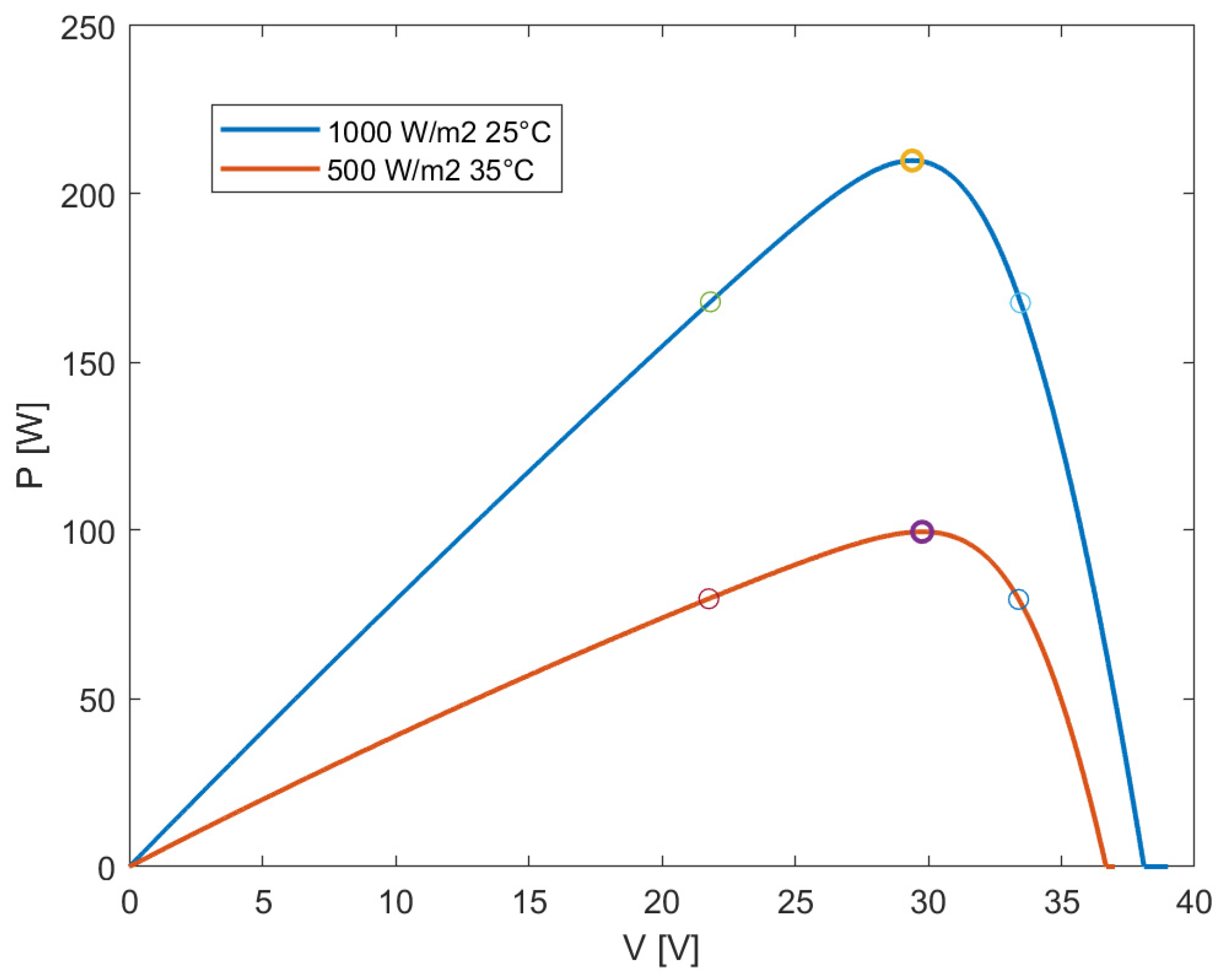
The concept presented in the following is the basis for all the power curtailment methods. It is based on the imposition of a certain level of active power required from the plant (Pres), that has to be reached by modifying the voltage applied to the PV panels (vPV*), taking into account the power-voltage curve, as shown in Figure 1.
It is evident that, given a certain Pres, it is fundamental to characterize the irradiance (G) and the temperature (T) in order to establish the shape of the power curve. In this sense, this raises another problem: the choice of the method to obtain the power curve. Different solutions are available, for example, the direct measurement of G and T, a non-linear least-square curve fitting or using solar forecasting methods. The choice represents a trade-off between cost and accuracy, due to the fact that the most accurate methods are also the most expensive to be implemented. Once the actual current-voltage curve is determined, all the inputs required for the algorithm are available:
  • If PresPMPP → MPP operation: the PV system will operate at its maximum power point, so vPV* = vMPP and PPV = PMPP.
  • If Pres < PMPP → curtailed operation: the PV system will operate at a voltage vPV* = v and PPV = Pres.
It can be noticed that, in the curtailed case, two voltage levels are possible for the same Pres, respectively, on the left and on the right of the MPP: a comparison between both options is provided in the following.

1.2. Power Ramp-Rate Control (PRRC)

The aim of this strategy is to smooth the active power output oscillations of the PV system. In particular, the algorithm imposes a maximum rate of variation of the active power output when variations of irradiance occur. In this case, the criterion to curtail the power does not come from the absolute value of the active power output but from its change rate with time [12]. The PV power ramp-rate can be calculated as in Equation (2):
Rr(t) = dPpv/dt
If Rr(t) is higher than the limit value required by the system operator, the voltage vPV* is perturbed in order to reduce the change rate of the PV power to that value. This kind of control can be performed both by controlling the voltage (as just explained) or the power.

1.3. Power Reserve Control (PRC)

This control logic can be seen as a particular case of the PLC algorithm. In fact, instead of imposing a certain constant power output level, in the PRC algorithm the PV output is regulated as a percentage of the maximum available power in each time instant. This dynamically changing fraction of the MPP is called Power Reserve (∆P). The output power is then obtained as:
Pres = PMPP − ∆P
Additionally, in this case, the challenge is to estimate the MPP, since it is one of the inputs necessary for the controller. The detailed explanation of this algorithm as well as of the determination of the power-voltage curve (and so of the MPP) is provided in Section 2, where the complete implementation of a model to control the active power output of photovoltaic modules in order to enable their capability to participate in the primary frequency control is described.
This work is focused on the third solution. To better organize the literature review regarding PRC, the differences between approaches are outlined under some key aspects: PV plant model, estimation output, controlled variable, MPP tracking method, and operational side of the power-voltage curve. The summary of reviewed articles is presented in Table 1.
The starting point of each work about the power reserve control of a photovoltaic grid-connected system is the model adopted for the plant itself. There are two main approaches: the most complete one is the two-stage model [18], which comprehends all the conversion stages between the modules and the grid. It includes the boost converter to step up the voltage to the DC-link value, the inverter, and an LCL filter. However, since the actual power output control is operated on the DC-DC converter, the single-stage model is the most commonly used in the literature, as represented in Figure 2, where the duty cycle command is obtained using a control module. The main differences between all the reviewed methods are found in this control module.
The logical process of the control block is a sequence of some key operations. First of all, the maximum power point is estimated in real-time. This calculation can be performed through a variety of techniques. The approach proposed in [13] is probably the most widespread: the power-voltage curve is estimated from past measurements of power and voltage, in the current window close to the operating point, through the equation for the power-voltage curve shown in Section 2. The measurements are referred to the last temperature value recorded and fitted through a least-squares curve fitting method, whose output are the five characteristic parameters of the module, as presented in Section 2. Qualitatively, without entering in the detail of the mathematical formulation, which is not the focus of this paper, the least squares fitting consist in finding the power-voltage curve that best approximates the measurements, i.e., gives the lowest difference between the measurements and the estimated values. A similar approach is used in [14], but with a combination of a linear and a quadratic approximation. The interesting aspect of [14] is that, focusing on multi-string PV plants, one string called “master string” is operated at the MPP, but using the estimation of the MPP of the master as reference, while the others are in the curtailed mode. A non-linear least-squares fitting is also used in [17], proposing further and deeper observations about the possibility to follow the actual characteristics of the PV modules when temperature and irradiance change, and demonstrating that the non-linear least squares fitting works well also in changing ambient conditions if measurements close to the MPP or on its right are used. Since the current-voltage curves of PV modules are almost superposed for different temperatures on the left side, it is not possible to estimate the correct one if measurements are taken on that side. However, since the temperature dynamics are slower than the irradiance one, it is possible to operate with measurements on the left side, at least for short periods. A different method is used in [16]: the MPP is found using a polynomial function of the irradiance and the temperature, which in this case, differently from the previous ones, are measured. The coefficients for the polynomial relation are found by calculating the value of the module current (with Equation (7)) for all the expected irradiance, temperature, and voltage values, then numerically finding the power maximums and interpolating them with a linear regression. It is also worth stating that, in photovoltaic systems, another possibility to find the MPP are the Perturb and Observe methods [19], representing the traditional methods of estimation, which in this case are not useful since the knowledge of the entire power-voltage curve is necessary.
Once the MPP is known for the actual operating condition (so for an irradiance/temperature pair) the required operating point to deliver the curtailed active power output desired has to be calculated. The most used control variable is the PV voltage: the voltage level corresponding to the desired output power is calculated and then it is compared with the actual voltage applied to the PV system to produce a duty cycle signal by means of a proportional-integral (PI) controller. This approach is used in [14,16,17]. The same reasoning is adapted with the power as a reference variable in [13,15], where the desired value of power is compared with the actual value to produce a duty cycle signal for the boost converter.
It is also important to notice that, for a certain level of curtailed power desired, there are two options in terms of voltage, respectively, on the left and on the right side of the maximum power point in the power-voltage curve. The scientific literature does not agree on which is the best side of the power curve of the PV module to operate the power curtailment. All the existing algorithms work only on one side. Since the operating condition throughout the year can be very different, this can be limiting.
In fact, operating on the right side allows a bigger variation range of the power, but at the same time modest reductions in irradiance can lead to a drop in the power output. This behavior can be easily explained looking at the characteristic power-voltage curve shape: reasoning at fixed irradiance, a request of power reduction from the system operator can be easily satisfied with small variations of the operational voltage. This is intrinsic to the high slope of the right part of the power-voltage curve. On the contrary, in a context in which the irradiance variates a lot, if a reduction in irradiance occurs at constant voltage the power output would immediately reduce, and even become null.
Instead, on the left part of the curve the pros and the cons are shifted due to the lower slope of the curve: there is a moderate insensitivity to the irradiance, but at the same time the range of variation of power is very restricted.
From these observations, it can be immediately pointed out how the choice of a single side of the power-voltage curve for power curtailment can influence the actual capability of the plant to participate in frequency control. In this sense, it becomes crucial to develop an algorithm able to adapt the control strategy to the boundary conditions of the problem (i.e., meteorological conditions, level of power reserve demanded by the system operator) [17]. This is why the present work adopts the approach proposed in [17], to be able to work on both sides of the power-voltage curve, exploiting the advantages of the operation on the two sides as a function of the situation.
Together with the photovoltaic technology, wind turbines are certainly the most exploited solution to drive the energy sector through the decarbonization. For photovoltaic systems, the algorithms to control the active power output through the power reserve control are relatively similar to each other in the logical sequence, but for wind turbines this does not happen. Indeed, there are different techniques to provide inertial control and, in particular, primary frequency control. The large variety of solutions is well described in [20]. Primary frequency control with wind turbines is an autonomous response to a change in system frequency that emulates the governor control of synchronous generators. More precisely, when a change in frequency is detected, the wind turbine modulates its power output to respond to this change and help to balance the system. Figure 3 summarizes different categories of methods for inertial control and primary frequency control in wind power plants.
First of all, it is important to offer an overview of the different types of wind turbines present in the market. In general, there are fixed speed wind turbines, semi-fixed speed wind turbines, and variable speed wind turbines (VSWT) [20]. Fixed and semi-fixed speed turbines have an inertia constant but are smaller with respect to the conventional synchronous generator ones, due to the lower coupling of induction generators with the grid frequency. This makes their inertial response lower and slower compared to the conventional generation [20]. On the other hand, as already mentioned, variable speed wind turbines (which are dominant in the market due to their higher efficiency) are decoupled from grid frequency due to the presence of the power electronics converter, so their contribution to the system inertia is null. However, it is possible to achieve a short-term inertial response from VSWTs by introducing an additional control loop in their control system. This control modifies the operation, allowing the turbine to exploit the kinetic energy of its rotating mass to modulate the electrical power output of the system and so to contribute to participation in the inertial control.
The functioning principle is simple: if the control detects a frequency variation, a signal is sent to the turbine speed governor or torque governor, temporarily modifying the power setup according to the magnitude of the frequency variation and enabling the possibility to exploit an amount of the kinetic energy of the rotor. For example, if an increase in power output is required to balance a frequency decay, the kinetic energy stored in the rotor is temporarily released. In this case, an unbalance between the electrical power injected into the grid and the mechanical power extracted from the wind is created, causing a deceleration of the rotor (i.e., a decrease in kinetic energy). This slowing down reduces the lift, discharging aerodynamically the blades, and increasing the stall risk at the bottom sections of the blade. To avoid stalling, the overproduction period has to be followed by an underproduction period in which the rotational speed of the rotor is increased [20].
There are different models for the inertial control described in the literature, but they can be conceptually divided into two main categories: a “simple” inertial control, which takes into account just the absolute value of the frequency deviation ∆f or the frequency derivative df/dt, or an inertial-droop control, which takes into account both. The first category is presented for example in [21,22], while the second is adopted in [23,24]. The inertial-droop approach allows for a very fast inertial control as well as an active power support more extended in time. An extended explanation of this kind of control is given in Section 2, since is the one adopted in the present work. The droop concept for VSWTs is analogous to the synchronous generators one. There are two main types of droop control: fixed or variable droop value. The second is more accurate in responding to frequency deviations, since it depends on wind and power reserve conditions [25] or on the RoCoF [24,26]. Indeed, it ensures improved system stability and avoids reserve exhaustion. The drawbacks of this kind of control are intrinsic to the physical behavior of the rotor during frequency oscillations. In fact, when the rotor slows down, it has always to respect aero-mechanical limits and avoid stall, keeping a safety margin; consequently, the control is limited, especially for low wind speeds. Furthermore, while the operational life in normal operation has been extensively tested at industrial levels, the operation with inertial control enabled has not, leading to the prescription of a practical utilization of this kind of control in only a few situations by the grid codes [20]. Another issue is related to the fact that, to re-accelerate to optimal speed, the power released to the grid has to be lower than the one coming from the wind. This implies that, for a certain time interval, the power output of the turbine is lowered to recover kinetic energy, delaying frequency recovery and, in some situations, requiring an extra number of reserves to prevent a “double-dip” in system frequency, increasing the risk of triggering protective relays at the substation level and causing blackouts [27].
In normal operation, wind turbines follow the MPP to extract the maximum energy available from the wind, achieving the highest aerodynamic efficiency possible. However, if an underfrequency event happens (i.e., the load increases its power), with such an operation there is no margin to respond to the frequency variation. On the other hand, through de-loading, the operation is shifted from the maximum power point to a sub-optimal one, keeping a power margin to face that event [28]. To work in a de-loaded condition, it is sufficient to reduce the coefficient of performance of the turbine (Cp), which is a function of the tip-speed ratio (λ) and of the pitch angle (β). The tip-speed ratio is proportional to the rotor rotational speed (ωr). Consequently, it immediately derives the two possibilities to de-load the wind turbine: working in a rotational overspeed condition (as in [29]) or through a pitching control. Usually, rotor overspeeding is applied when the rotor speed is low, while for a rotor speed equal or higher than the rated one the pitch control technique is used [30]. The de-loading of wind turbines has some limitations that historically confined it to very few practical applications. First of all, similarly to what happens in the power curtailment of photovoltaic plants, the de-loading leads to a reduction in the annual capacity factor of the turbine. At the same time, overspeeding can reduce the turbine’s life. To determine the power set-point, accurate wind speed measurements are important, otherwise incorrect or rough estimations can highly affect power output and turbine life [20].

2. Model for a Small Island Power System with Renewable Generators Participating in the Primary Frequency Control

After an overview of the techniques that allow the considered renewable generators to participate in the inertial and primary frequency control, it is important to go through the model developed in this work.
The negative effects on stability due to a massive presence of variable renewable sources are more severe in small and isolated power systems, due to a lack of interconnections with other systems and to their limited inertia. For this reason, many studies have assessed the impact on the frequency stability in small island power systems [29,31]. In this work, a generic small island power system has been considered, i.e., the most challenging situation, to evaluate the coordinated effect on frequency stability of photovoltaic modules equipped with a power reserve control and wind turbines with inertial control enabled. The models described in the following have been developed using the Matlab/Simulink software, which allows for easily the observation and study of a large variety of scenarios.
This section starts with an overview of the complete model to offer a general introduction to the problem and it continues with the detailed description of the different subsystems of the model.

2.1. Assumptions of the Model

Before starting to describe the model, it is important to state the fundamental assumptions on which it is based, which are necessary to understand the work and its main objectives.
The most important observation regards the power system representation: in primary frequency control studies, i.e., in the time frame from 1 to 100 s, it is a common practice to schematize it using the Load Frequency Control (LFC) approach. In fact, in such problems, the time constants of the electromechanical variables are much smaller than the ones representing the dynamics of the mechanical variables of synchronous generation prime movers [32]. Furthermore, the time constants of the wind turbines and photovoltaic converters are very small, justifying this approach [24]. Due to this reasoning, the equivalent inertia constant of the system is the key parameter to obtain the dynamic frequency characteristics [33], together with the load damping constant, which describes the sensitivity of load power to the frequency variations [32]. This allows for the representation of the entire system response just through a transfer function block, making the problem at the same time easier to be modeled (the system is not modeled node by node) and more general. A similar kind of reasoning is related to the generation blocks. Indeed, since the only aim of this work is to observe the inertial and the primary frequency responses, each single generating unit is not represented, all of the same type are aggregated in equivalent generating units. This is valid in particular for the variable speed wind turbines and for photovoltaics. The same principle is applied to the load, which is schematized as a unique block. The main advantages of this approach are the simplicity and the versatility of the results to a lot of practical cases, while the main drawback is the losing of detail.
To account for the penetration of the different generating sources in the energy system, a participation factor (pi) is used, which represents the fraction of the total power of the system which is generated by the i-th source.
Other assumptions, which are quite usual in this kind of study, are related to the ambient conditions. In the simulations, the effects of variable wind speed, variable irradiance, and ambient temperature are considered. At the same time, the non-uniform distribution of the wind resources among different wind turbines is neglected, since they are considered as an aggregate; the same happens for photovoltaic modules, which work under the assumption of uniform radiation, and shading is neglected.

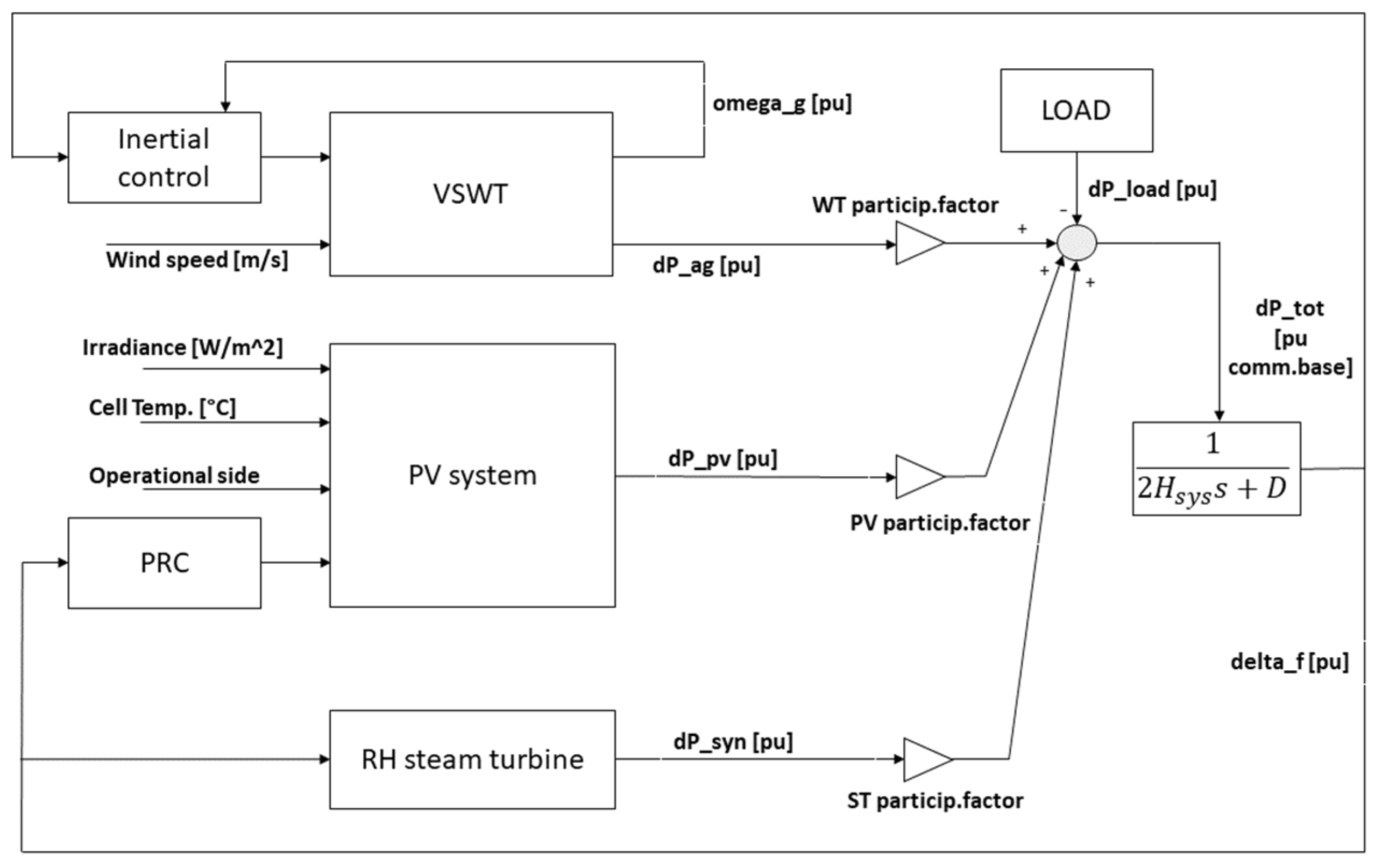
2.2. Overview of the General Model

The upper layer of the model of the system under study is shown in Figure 4. It represents a small isolated power system, comprehending three kind of generating plants: a reheated steam turbine, wind turbines and photovoltaic units. It has to be specified that the total generated power (that in equilibrium condition equals the load power), as well as the power of the three generating blocks, vary with the magnitude of the participation factors. In fact, in this kind of study, the importance is related to the relative weight of the three generating blocks rather than to the absolute magnitude of the system, since it is based on per unit variations in a reference common basis. This concept is particularly relevant for simulations at different participation factors, as the ones presented in Section 4.
Before going deeper into the characteristics of the different subsystems present in the model, it can be useful to understand the main connections between them, to facilitate their study. Each of the three generation blocks produces a signal of variation of power in per unit with respect to the steady state value (dPi), which is the power corresponding to the initial condition:
Pi,0; Σi (Pi,0) = Pload,0
Indeed, all the simulations are initialized to have a dPi [pu] = dPload [pu] = 0, corresponding to a frequency value equal to the rated one, which is 50 Hz (i.e., ∆f = 0).
The three signals of variation of power of the generating blocks are initially in per unit with respect to the generator nominal power, so they require to be weighted to obtain the equivalent variation on a common basis (the sum of the nominal powers of the three generators blocks): each of them passes through a gain block in which it is multiplied by its participation factor, as in Equation (5). The dPload, on the contrary, is already defined in per unit common basis.
dPi[pu_common basis] = pi dPi[pu]
For simplicity, from now on, “common basis” is omitted in the equations. Then, the four dP signals are summed up to obtain the instantaneous power unbalance of the entire system:
dPtot[pu] = Σi (dPi[pu]) − dPload[pu]
A non-negative power unbalance leads, through a transfer function, to a frequency deviation from the nominal value. The transfer function describes the frequency response behavior of the system. The meaning is captured by two parameters: Heq is the equivalent inertia constant of the synchronous generator present in the system, and D is the damping constant of the load, which represents the sensitivity of the load power to the frequency variations. The function output is the signal representing the frequency variation in per unit with respect to the nominal value, which is also one of the metrics to evaluate the system behavior in the analysis presented in Section 4. The frequency variation signal is also the main input to the controllers of the three generators. Indeed, the synchronous one is traditionally able to respond to a change in system frequency by adapting its power output, but in this study also photovoltaics and wind turbines are, thanks to the presence of the power reserve control block (PRC) and the inertial control block, respectively.
After this brief introduction, a more detailed analysis of each block is required, to understand the modeling of the generators as well as the functioning of the above-mentioned controllers.

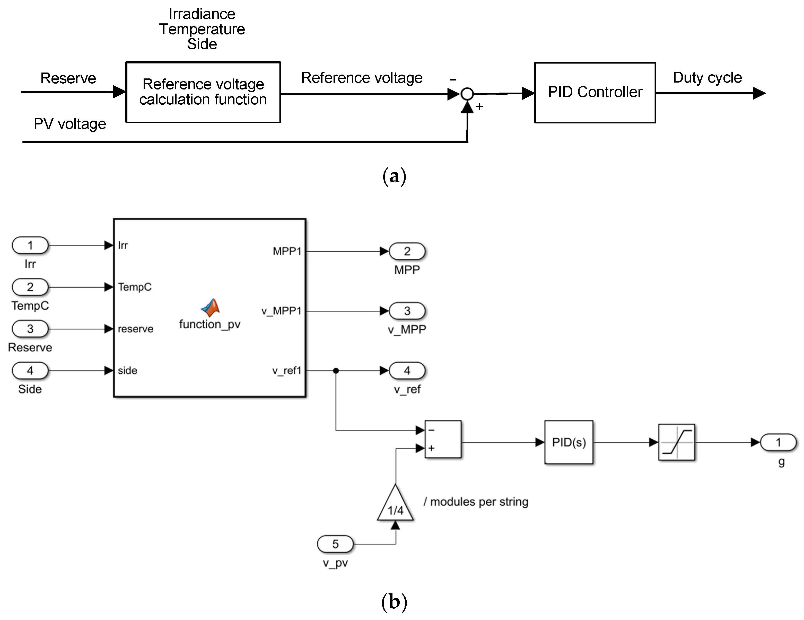
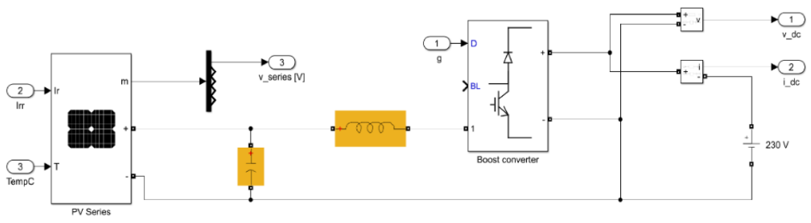
2.3. Photovoltaic Generators Model

One of the three generating blocks represents the photovoltaic modules present in the system. The modeling of this block is quite challenging, requiring a lot of different literature sources as well as customized solutions to improve its functioning. Figure 5 gives an overview of the model.
The model is divided into two subsystems: the upper one contains the electrical model of a photovoltaic string, while the lower block represents the control system of the PV string modified to implement the power reserve control. Observing the inputs, some observations can be performed:
  • Irradiance and cell temperature are the two ambient conditions that mainly influence the performance of the photovoltaic modules. They are assumed to be measured in real time: this is a strong assumption, which implies higher costs with respect to other solutions such as non-linear least squares fitting methods. This assumption comes from the fact that the aim of this work is centered on the control logic, not on the determination of the irradiance and cell temperature.
  • The reserve signal is produced by another subsystem that is presented in the following. It is sensible to frequency variation: if the frequency is at its nominal value, the reserve level is fixed at a certain value imposed by the steady state conditions. When the frequency oscillates, the reserve level is adapted automatically to face this variation. Of course, this signal is required by the control system to calculate the operating PV string voltage corresponding to a curtailed operation.
  • The last external input, indicated with Side, represents the desired operating side of the power-voltage curve for implementing the reserve control. In this work, the innovative approach proposed in [17] has been adopted, which allows, depending on the requirements, to operate on both sides of the power curve, by simply switching this input value.
The control system receives these four inputs, as well as the measurement of the actual voltage applied to the PV string, and calculates the maximum power point, the corresponding voltage, the reference voltage to operate in the desired curtailed condition and, above all, a duty cycle signal for the boost converter necessary to impose that desired operation to the PV string.
The general diagram of the voltage control subsystem is shown in Figure 6.
This subsystem is mainly composed of a function and a PID controller. The function is the most important element of the PV system, since it contains almost all the features that characterize the PV model proposed in this work. For this reason, it is appropriate to explain how the function works to obtain vref, i.e., the control variable of the PRC.
The first aim of the function is the determination in real-time of the power-voltage characteristic of the module. As already observed in Figure 1, there is a strong dependence of the shape of the power-voltage curve on the environmental conditions. This means that the model has to properly account for this fact. Two of the characteristic parameters present in the datasheet of all the photovoltaic modules, the open-circuit voltage (Voc) and the short-circuit current (Isc), participate in solving the equations and are impacted by irradiance and temperature. This means that, to be precise, they have to be adapted to the actual environmental conditions. In the literature, different approaches are proposed to do so, which are reviewed in [34]. In this work, the following correlations have been used:
Isc = Isc,ref G/Gref [1 + αsc (TcellTcell,ref)]
Voc = Voc,ref [1 + βoc (TcellTcell,ref)] + 54.68511∙10−3 log(G/Gref) +
  5.973869∙10−3 log(G/Gref)2 + 761.6178∙10−6 log(G/Gref)3
The Single-Diode Model (SDM) of the photovoltaic cell [35] adopted in this work is characterized by five parameters: Iph,cell (also called IL) is the photocurrent, Is,cell is the saturation current of the diode (also called I0), n is the diode ideality factor, and Rs,cell and Rsh,cell are the series and shunt resistances, respectively. The electrical variables of interest are the PV cell terminal voltage (Vpv,cell) and current (Ipv,cell) [35]. The parameters solve the implicit equation describing the current-voltage characteristic of the cell (which is extendable to the module):
I = I L I 0 { exp ( V + R s   I n   V t h ) 1 } V + R s   I R s h ,
where Vth is the thermal voltage. In principle, all the parameters necessary to solve the equation can be calculated numerically as in [35]. On the other hand, to estimate IL and I0, Equations (10) and (11) can be used, respectively [35]:
I L R s + R s h R s h I s c ,  
I 0 ( R s + R s h ) I s c V o c R s h exp ( V o c n   V t h ) .
Once the current is known for each voltage between 0 and the actual Voc, the power curve is easily obtained as the product between it and the corresponding voltage. Once the power-voltage characteristic is known, the maximum power point can be easily extracted, as well as the corresponding voltage level. Indeed, the MPP is found as the maximum of the power-voltage curve. In the last part of the function, the reference voltage for the power reserve control is found. In particular, knowing the desired reserve amount, it is possible to calculate the corresponding power. Once this is known, an operational side of the power curve is imposed through an external signal, determining the reference voltage (vref) thanks to a simple minimization problem and finding the voltage vector element on the desired side, which corresponds to the calculated curtailed power.
The reference voltage signal is then compared with the actual voltage applied to the module. The associated PI controller acts on the duty cycle signal to minimize the difference. Indeed, the output signal of the voltage control subsystem is the duty cycle, which is imposed to the DC-DC boost converter in order to set the module (the series) voltage to the desired value.
The second subsystem forming the photovoltaic system block is the one containing its electrical model, which is in practice the object of the control subsystem’s operation. It is basically composed of a PV array in parallel with a capacitor and a boost converter. The DC-DC converter connects these elements to a DC-link, whose voltage for the aims of this work is assumed to be fixed to 230 V, as common practice in the literature when studying the power reserve control of a PV system [17]. In practice, the single-stage PV model already mentioned (as shown in Figure 2) has been used. The corresponding Simulink implementation is the subsystem diagram presented in Figure 7.
To fully describe the photovoltaic system, it is necessary to specify another aspect: how the adaptation of the active power output happens in response to a frequency change. This is implemented partially in the voltage control block, but to close the loop, it is important to notice how the reserve input signal is generated. The reserve adaptation block (PRC in Figure 4) receives the per unit frequency deviation as an input. The reserve is adapted through a droop characteristic so that the output variable is changed proportionally to the input one. In this case, the reserve is increased if the frequency increases, i.e., the power produced is reduced by working away from the MPP.
It is fundamental to set a proper droop value. To do so, extensive tests have been performed. On the one hand, a too high droop constant means that the reserve varies very slightly, providing insufficient help to the primary frequency control. On the other hand, a too low droop constant leads to a reserve depletion or to an extremely low power production. As a compromise, a value of 0.05 has been used, which is identical to the droop constant of the synchronous generators presented in the following of this work.
The rest of constants used can be found in the Appendix A.

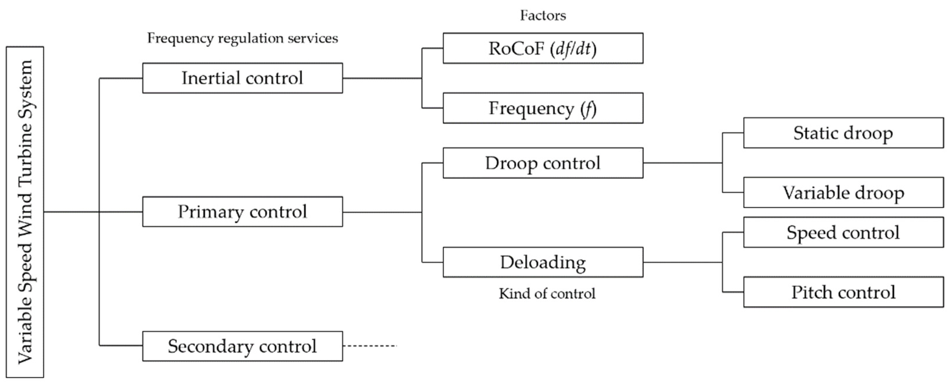
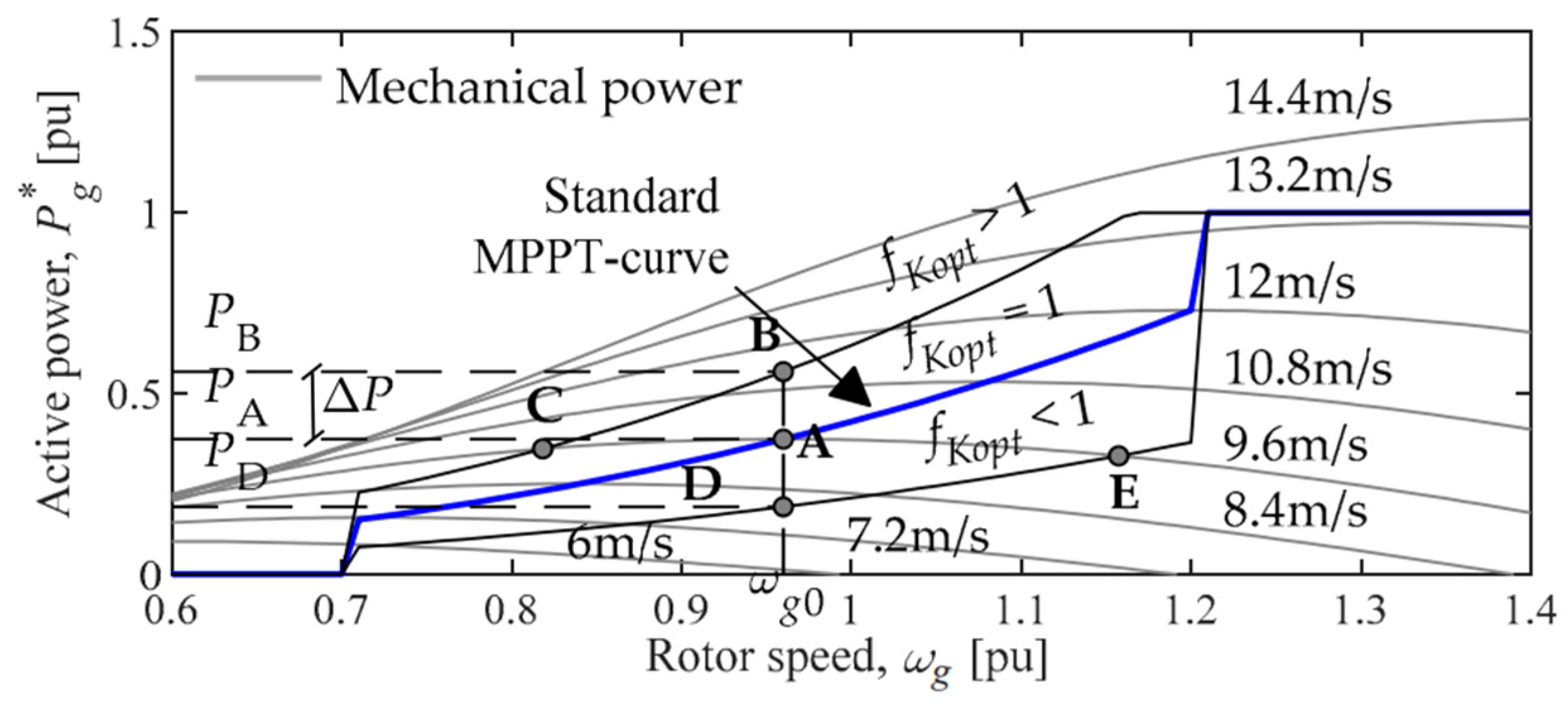
2.4. Variable Speed Wind Turbines Model

There are many different solutions when designing a wind turbine. For example, there are several types of generators that can be coupled to the rotor. In this work, a variable-speed wind turbine using a DFIG (doubly fed induction generator) with pitch control enabled has been chosen as representative.
The block diagram of the model is presented in Figure 8 [36]. This layout is formed by five subsystems interacting with each other. Following a conceptual path from the wind speed to the output power: a predefined Simulink wind turbine block, which receives the wind speed, the low-speed shaft rotational speed, and the pitch angle signals and calculates the mechanical torque applied to that shaft; this torque signal is compared in the mechanical system (which represents the gearbox mechanisms) with the torque applied to the DFIG generator and the rotational speeds of the two shafts are calculated through a first-order dynamics represented by a transfer function; the high-speed shaft signal is used in the speed governor block to calculate the new power setup, compared in the same block with the actual power to calculate the reference generator torque; in the DFIG, simply modeled through another first-order dynamics, the reference torque is imposed to the generator; and a pitch control block adapts the pitch angle, if necessary, as a function of the high-speed shaft rotational speed, to limit the output power to the maximum value for wind speeds higher than the nominal one.
The inertia control is grafted in this model inside the speed-governor block. In particular, a multiplication factor fK,opt (which is calculated in the inertial control block) called signal for the optimization zone is used to shift the operation of the wind turbine from the MPPT curve to other curves by exploiting the kinetic energy of the rotor (Figure 9). This method is called the Extended OPPT Method [24]. The control function of the method is shown in Equation (12). As can be observed, fK,opt depends both on the frequency deviation and on the time derivative of the frequency. Indeed, the effectiveness of this virtual inertia algorithm depends both on the magnitude of the frequency disturbance (through ∆fs and dfs/dt) and on the initial kinetic energy stored in the rotor before the disturbance.
fk,opt = [ωg0[pu]/(ωg0[pu] + kvirfs[pu])]3Wvir K0/(Kopt ωg0[pu]3) fs[pu] dfs[pu]/dt,
where:
K0 = 2 ωg0[pu]/ωs0[pu] kvir HWT,
and ωs0[pu] is the pre-disturbance rotational speed corresponding to the system frequency, 1 p.u.
The inertia control block simply implements these equations in a block diagram, providing the fK,opt signal as the final output, which, as already mentioned, is used to shift the operating point of the turbine.
Looking at the P-ω chart in Figure 9, it is possible to understand the functioning of the OPPT algorithm. Under the hypothesis of constant wind speed and normal operating conditions, the generator will deliver a power PA associated with a rotational speed ωg0. If an underfrequency event happens, caused for example by a mismatch between the injected and the consumed power in the system, an increase in the power output of the turbine will be required to reduce the frequency oscillation as much as possible. In particular, the non-null values of ∆fs and dfs/dt will activate the inertial response emulation of the wind turbine, with a consequent shift of the MPPT curve upwards (A → B). The higher the severity of the underfrequency event (and so the magnitude of ∆fs and dfs/dt), the higher will be the value assumed by PB. In this situation, the imbalance between the active power extracted from the electric generator and the mechanical power delivered at the turbine shaft will cause a deceleration of the rotating masses of the turbine, testifying to the exploitation of the turbine kinetic energy. This deceleration moves the operational point to the left (B → C), reaching a new equilibrium condition when PC coincides with PA; this is a situation that corresponds to a balance between the mechanical power delivered by the turbine and the active power extracted by the generator (PC). When the support is not necessary anymore, the system returns to the initial state (C → A), preparing it for future requirements [24].
Putting together these two renewable generators with a reheated steam turbine (modeled as in [32]), the scheme proposed before in Figure 4 is obtained, which is the one on which the following simulations have been performed.

3. Simulations Summary and Metrics to Evaluate the Results

To be as clear as possible, after showing the model layout, this section lists the simulations performed, with particular attention on detailing the aim of the different simulation categories and the metrics that will be used in next section to evaluate the results.
It is important to remember which situation this model is describing: a small island power system characterized by the presence of three equivalent generating units (PV, wind, and synchronous generator) and an equivalent load, which can be seen as a grouping of all the smaller loads present in the island. This situation, in fact, is the one in which a mismatch between the active power produced and consumed can have more serious effects on frequency stability, due to the small size of the power system, its lack of interconnections due to the remote geographic position, as well as the high penetration of renewable sources that is usually observed on the islands.
The simulations can be divided into some categories, as a function of the perturbation introduced with respect to a common reference condition. It is thus fundamental to describe this reference condition before going on. The common reference condition that has been chosen from now on will be indicated with “base case” and is characterized as follows:
  • Participation factors of the three equivalent generating units: pwind = 0.2; psynchronous = 0.7; ppv = 0.1 (30% of renewable penetration on nominal power basis).
  • Heq = 2.88 s [24]; D = 1 [32].
  • Incoming wind speed at t = 0 s: 9.6 m/s for constant wind simulations; 11.457 m/s for real wind profile simulations.
  • Irradiance at t = 0 s: 1000 W/m2.
  • Cell temperature: 25 °C.
  • Constant load power requirement.
In each simulation, a modification with respect to this base case is introduced to study different aspects linked to the frequency stability. As stated before, the simulations can be grouped as a function of the perturbation introduced. In particular, the situations compiled in Table 2 have been studied.
Furthermore, to have other points of view on the system, each simulation is performed on four different versions of the complete system:
  • Primary frequency control provided only by the synchronous generators (wind turbines without virtual inertia control, PV without power reserve control).
  • Primary frequency control provided by synchronous generators and wind turbines (Extended OPPT Method enabled).
  • Primary frequency control provided by synchronous generators and photovoltaic strings (Power Reserve Control enabled).
  • All the generators participate in the primary frequency control (from now on it is denoted as complete FC).
The first scenario is representing the current situation in most of the power systems, since the renewables are mostly operated in their MPP condition. The fourth scenario, on the other hand, could represent a future situation in which renewables are flexible and able to help synchronous generators (or displace them) in balancing the frequency of a power system. This captures the interaction between the various controllers, the help that the renewables controlled with the updated logics can provide to the system, and the impact of each technology in frequency stabilization.
The final summary of the simulations performed on the model is reported in Table 3 and Table 4. A number has been used to designate each of them, so that the results can be commented in a clearer way.
As is probably noticed, this work does not analyze the case of a generator loss. Indeed, this kind of model is not capable to catch that kind of event, excluding a loss of a part of the photovoltaic generation. This is intrinsic to the model developed for the system, in which the generators have to be intended as an “equivalent” of all the similar generating units present in the system. With some modifications, it is just possible to model the loss of the entire fleet of wind or synchronous generators. For PV, since a gain block is included at the output of the subsystem, it could be used to model a partial loss of generation.
Before presenting the simulation results, it is important to define quantitative instruments that can help in interpreting them. Indeed, the next section includes both qualitative analysis on the results and quantitative observations to catch some important concepts. It is first of all required to report a definition of primary frequency adequacy. As stated in [37], a primary frequency control is adequate if it is able to ensure an uninterrupted delivery of electricity after a sudden imbalance between generation and demand, i.e., if it is capable of arresting and stabilizing the frequency deviation without exceeding the limits imposed by grid codes.
In this work, the following metrics are used:
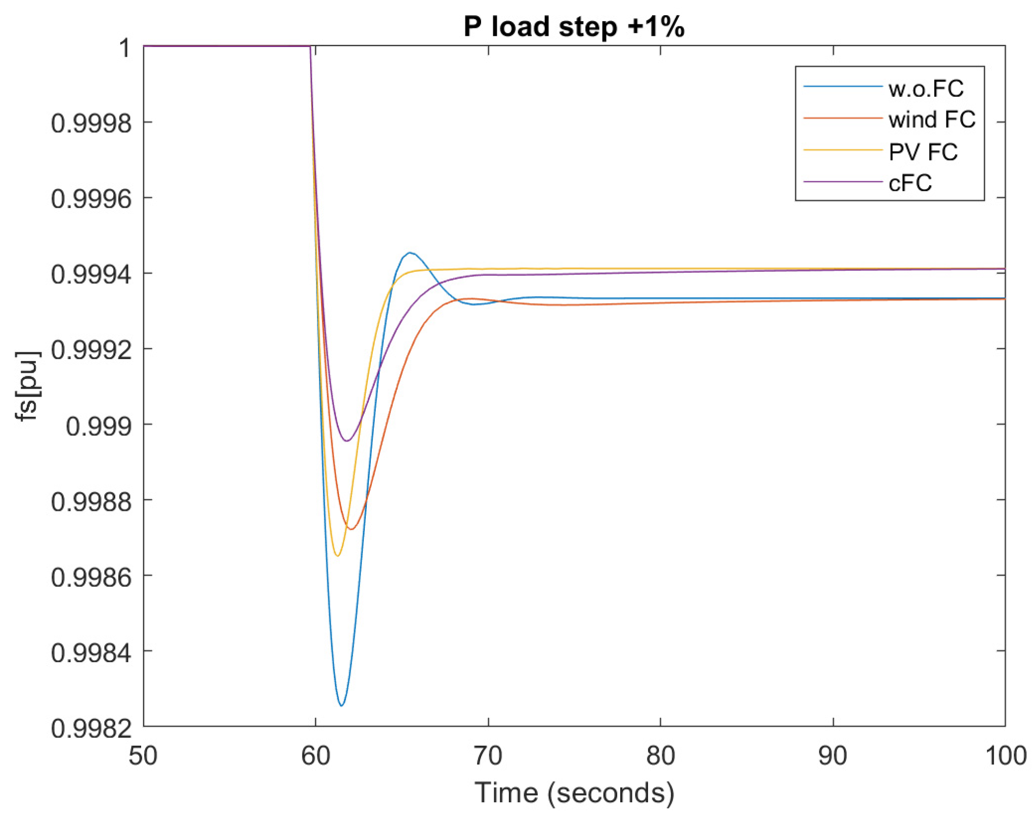
  • Frequency nadir [Hz]: it is a direct measure of the primary frequency control adequacy. It is calculated as the maximum/minimum value of frequency deviation occurring after an active power imbalance. The closer it is to the nominal frequency, the better.
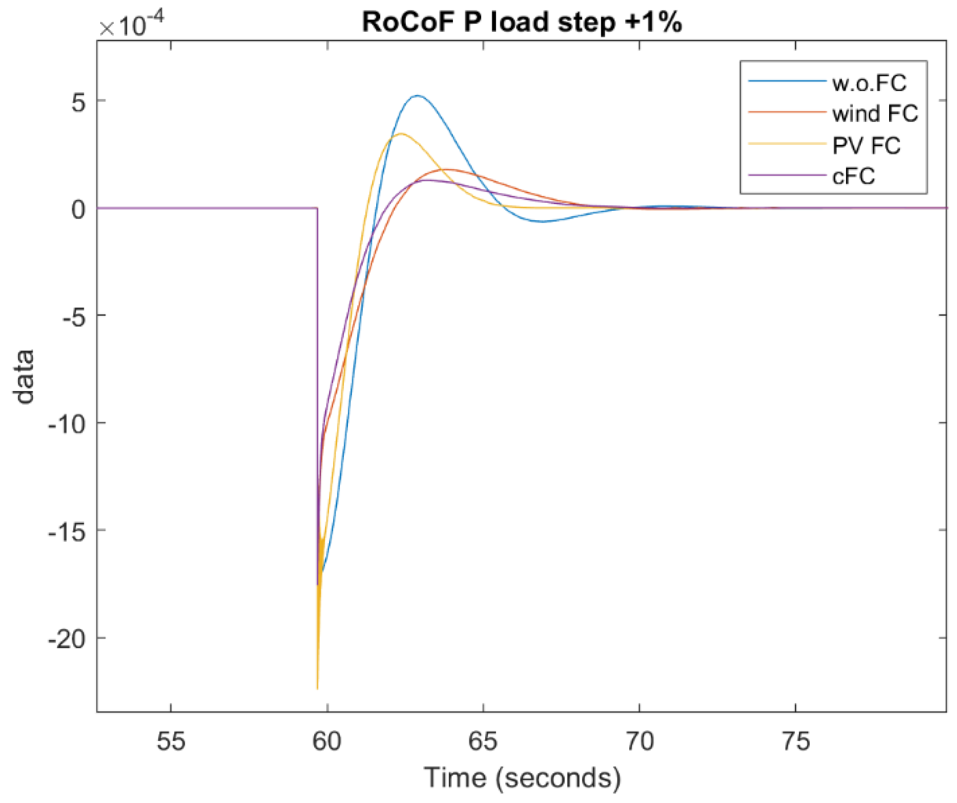
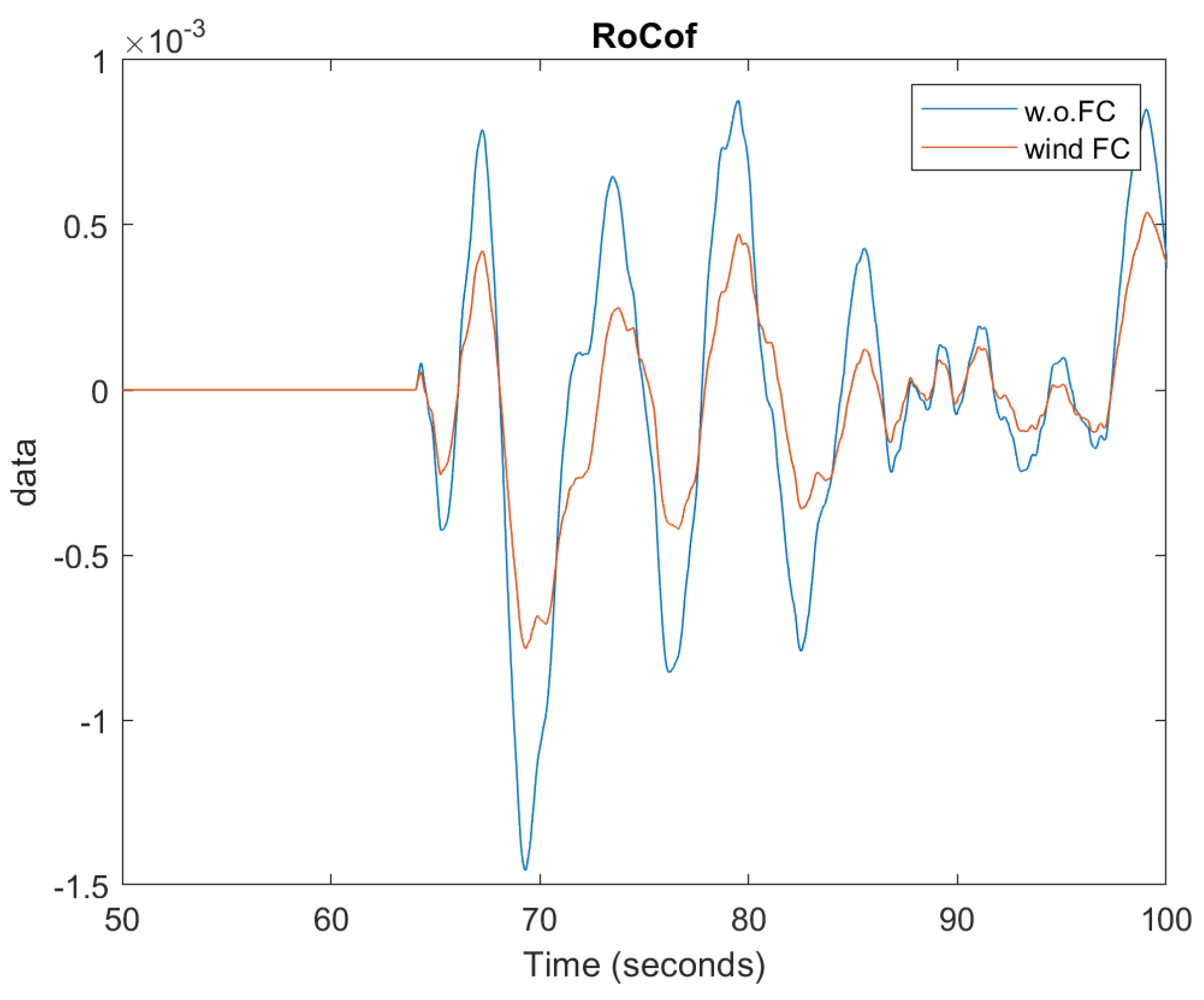
  • RoCoF [Hz/s]: it is the time derivative of the system’s frequency. The smaller it is, the better for the system.
  • Nadir-based frequency response: it expresses how good the primary frequency control has performed in stabilizing the frequency after a perturbation. It can be calculated as [37]:
Nadir-based frequency response = ∆Pperturbation/∆fnadir.

4. Simulation Results

Once the model has been presented in detail, it is now possible to finally match the modeling part with the conceptual part. Indeed, the previous sections have not addressed with quantitative and qualitative considerations the core of this work. It is interesting to approach the problem about the primary frequency control with some major questions: How the increasing penetration of renewable generators affects it? Is the possibility of including them in the provision of this ancillary service effectively helping the system and encouraging the displacement of conventional ones?
This chapter is trying to answer these questions both qualitatively, commenting some graphs, and quantitatively, thanks to the metrics proposed earlier in Section 3. For the sake of clarity, the results are divided and commented on by groups of simulations.

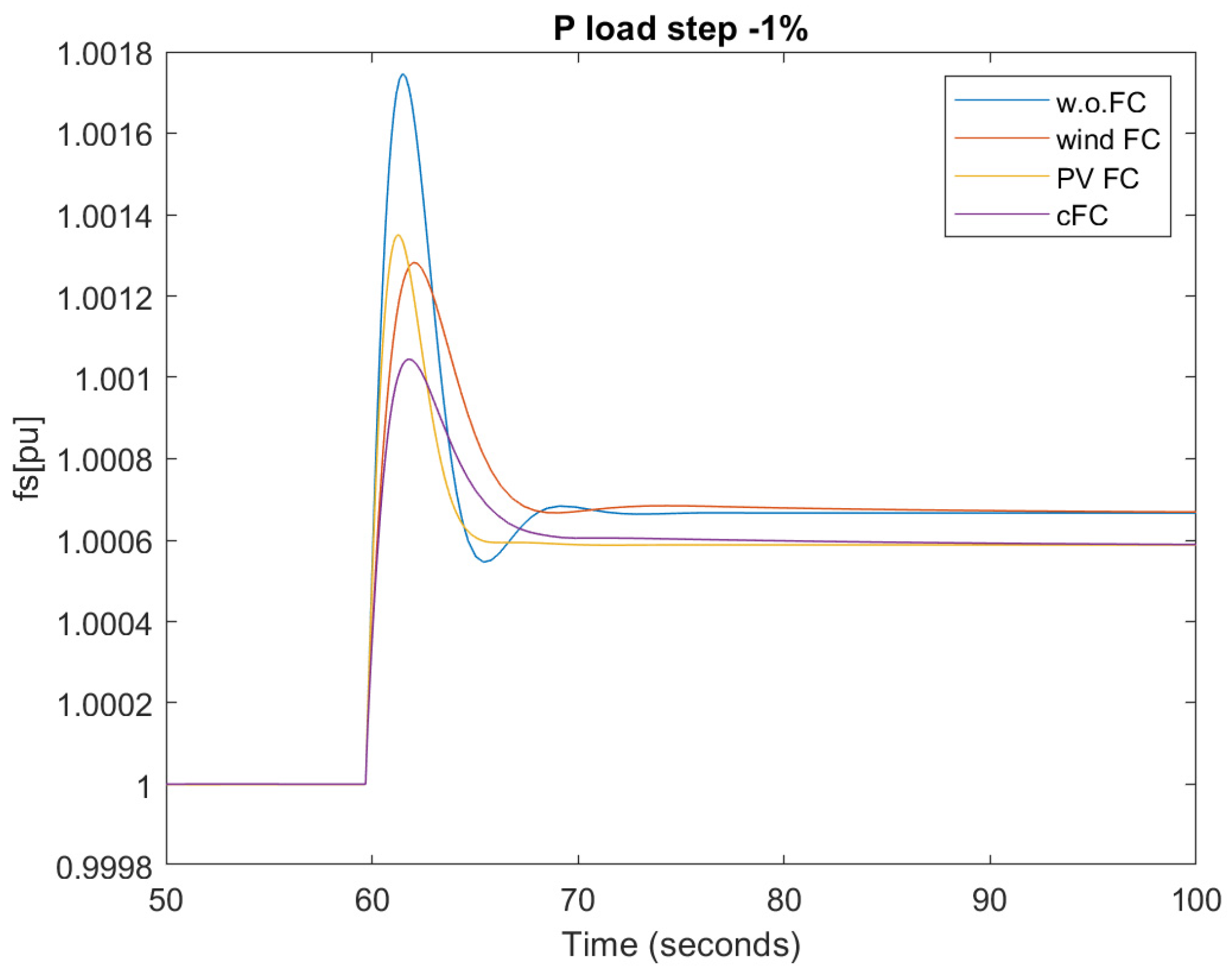
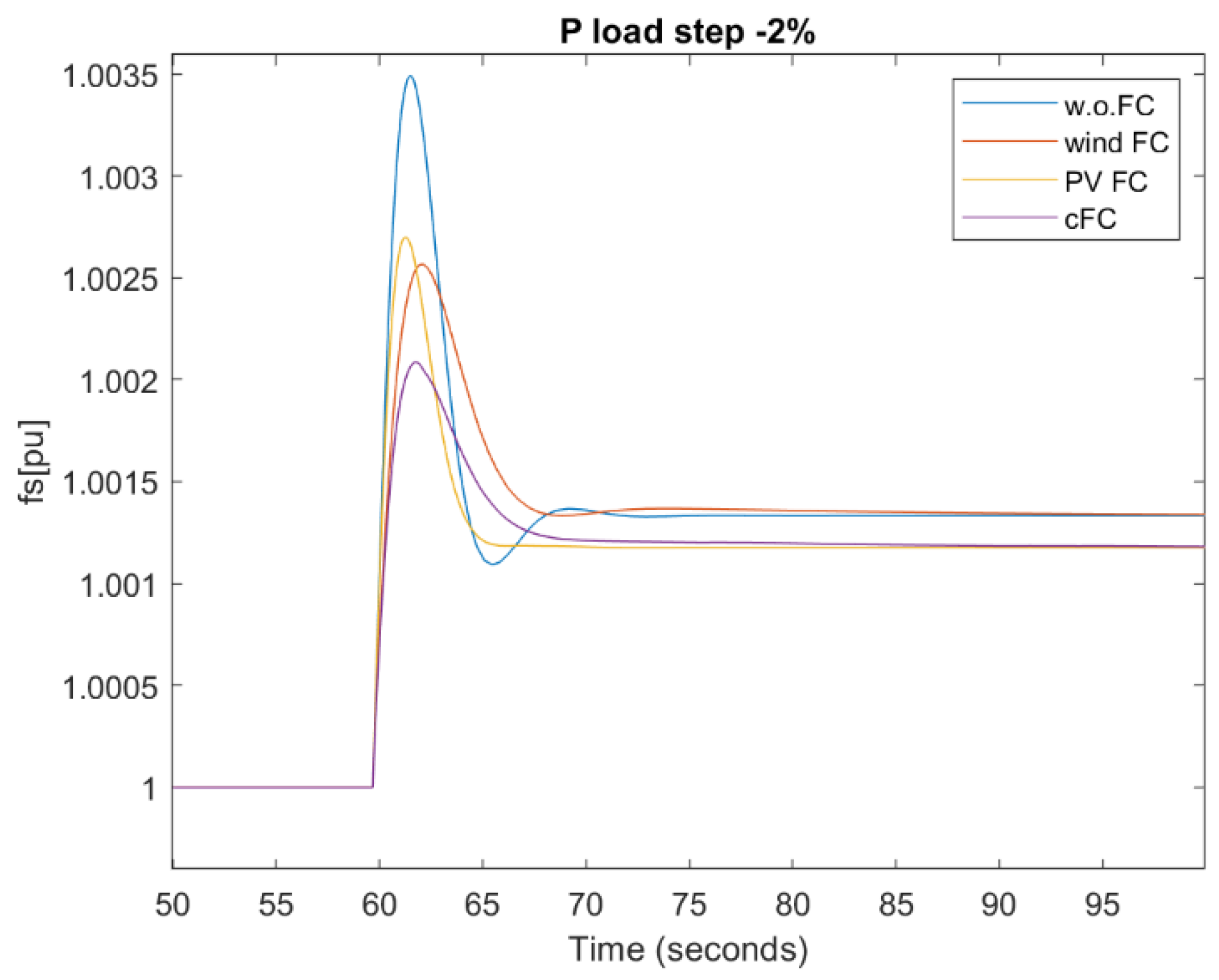
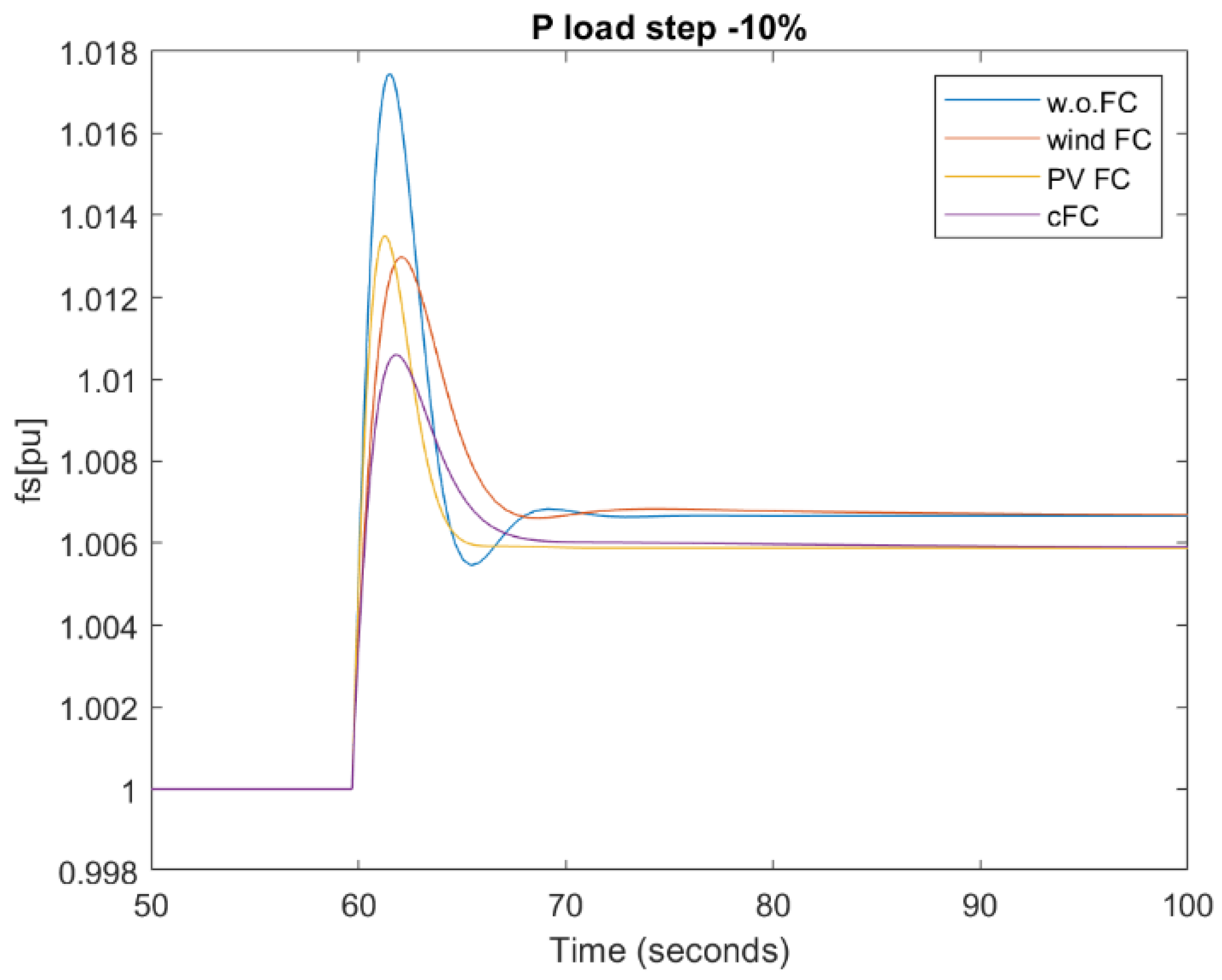
4.1. Load Power Step Up/Down

The first and simpler test to analyze the frequency response of a dynamic system is obtained by observing its behavior after a step perturbation. In this case, the step is an instantaneous change of the load power (Pload). This situation is extremely simplified with respect to what happens during the normal operation of a power system, but nevertheless this test is really important to take a first look at the effectiveness of the ability of the primary frequency control in stabilizing the frequency.
In the small island system that is described here through an LFC approach, a sudden step change of the load power is more likely to happen as a reduction. In other words, it is more common that the load decreases suddenly (for example due to a disconnection of an industrial user) than the vice versa. This is why the maximum amplitude tested for the steps in the reduction is higher than the one in the step up of the load power.
The first plot reported regards Simulation 1, in which the load suddenly increases its power by 1%. Figure 10 shows the frequency oscillation of the system due to the consequent imbalance between generation power and load power.
First of all, it can be observed that an increase in the load power causes a decrease in the frequency. In Figure 10, the frequency nadir can be easily individuated as the minimum of the frequency in the time plot. Observing it in the four scenarios: as expected, in the absence of frequency response capabilities from the renewable sources (w.o.FC), it is lower than in the other three scenarios. Indeed, it is equal to 0.9983 pu (49.915 Hz) against the 0.9990 pu (49.95 Hz) in case all the generators participate in the primary control (cFC). It is evident how the intervention of wind and photovoltaic generators in stabilizing the frequency is helping the system, since they reduce the magnitude of the nadir and, after a few instants, they also reduce the oscillations of the system’s frequency and the stabilization time. The superposition of their effects lead to the behavior in purple, which is one of the scenarios in complete FC, i.e., all the generators participate in the primary frequency control.
Of course, since this work focuses just on the primary (and inertial) frequency control, the final value of the frequency is not the nominal one, that requires also the actions of the secondary and tertiary control to be restored.
Looking at the RoCoF plot in Figure 11, it can be seen that the PV system produces oscillations that increase the RoCoF in proximity of the step. This is a negative fact, which would require an additional PRRC to be solved, that reflects also on the complete FC scenario. After the peak of the RoCoF, anyway, the scenario for which it is higher is the one without frequency control. This allows for the understanding that the PRC for the PV system is capable of containing the frequency and the RoCoF in the instants after a sudden variation in the load power. On the other hand, the wind virtual inertia operates very well both during and after the load power step.
Remarkably similar results are obtained from Simulation 2 as shown in Figure 12: a negative step of load power of the same amplitude produces the same behavior of the frequency but mirrored to an increase in frequency. The nadir is also simply mirrored upwards with respect to Simulation 1: in the scenario with the renewables with disabled frequency control, it is equal to 1.0017 pu, while for the complete FC it is equal to 1.0010 pu.
In the next simulations, larger steps are introduced. Due to the similarity already discussed between the first two, they are expected to produce a frequency waveform with the same shape but a different amplitude (dilated by a factor of 2 and 10, respectively). Looking at the results for Simulation 3 shown in Figure 13, this expectation is confirmed. This behavior is caused by the constancy of the load damping constant and of the inertia of the synchronous generator, which do not depend on the step amplitude.
It can be also observed that the time required to stabilize the frequency is practically independent on the step amplitude, since in all the simulations the new steady state condition after the load power step is reached almost at the same time instant.
These kind of results are coherent also with the plots for Simulation 4 shown in Figure 14. In this case, such a large loss of load could be associated with the disconnection of an industrial user, and it is evident how large the frequency variation associated with this loss is. The nadir reached in this extreme case is equal to 1.0175 pu (50.875 Hz), which is not compliant with many grid codes, for the “traditional” renewables control scenario. In the case of the updated control, on the other hand, the nadir is equal to 1.0106 pu (50.53 Hz), which also exceeds the upper frequency limit but is lower than the previous, highlighting the huge benefit introduced.
It is very interesting to observe how the different generators contribute to the frequency control by adapting their power, as shown in Figure 15.
It is clearly visible how the two renewables reduce their power to face a decrease in load. This helps the synchronous generator in containing the frequency increase: it can be seen that the steam turbine power reduction in the case of the complete FC is less intense than that in the case of the frequency control operated just by themselves. The stabilization effect is also emphasized by the reduction in the oscillations after the nadir, that further facilitates the intervention of the synchronous generator.
Considering the third metric (nadir-based frequency response), it has been shown with these numerical results that it is practically the same in all the four simulations for what concerns the conventional scenario, while in the case of the complete FC it is a little bit lower in increasing the step magnitude.

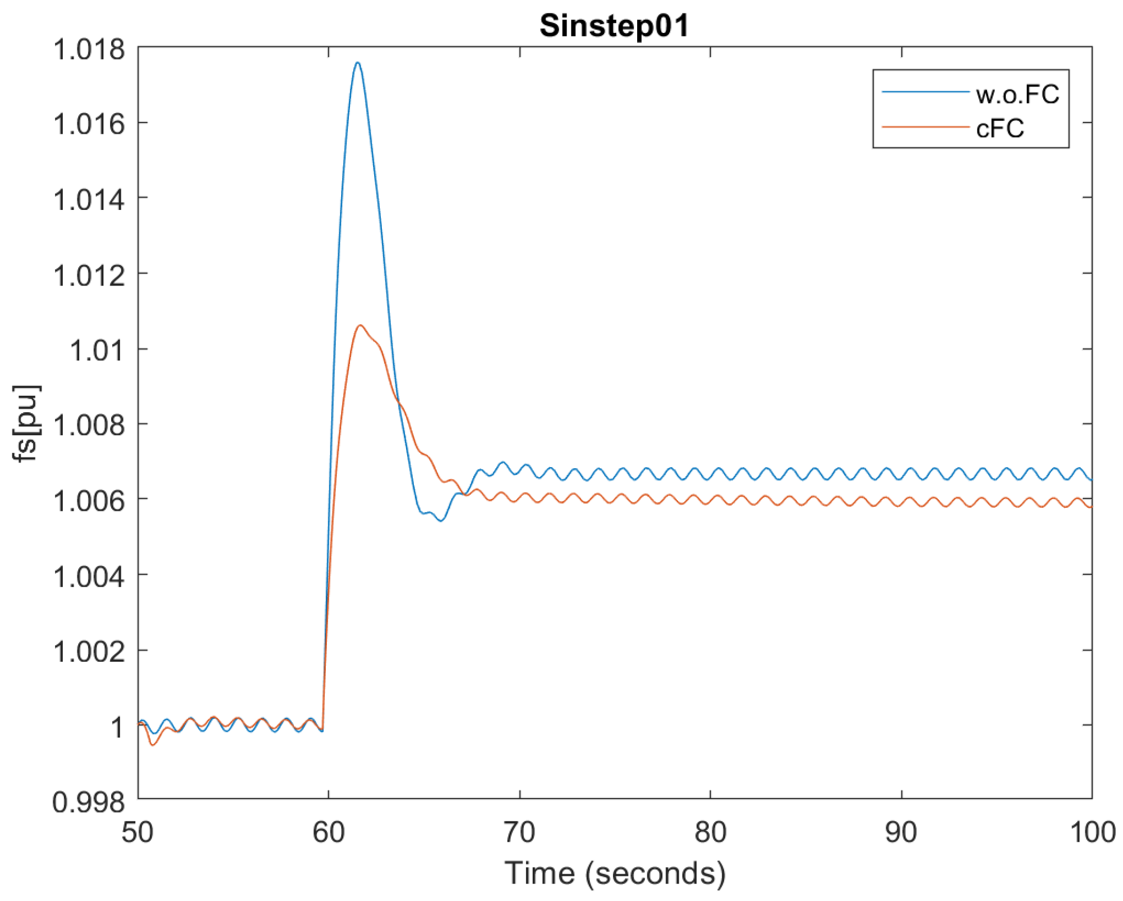
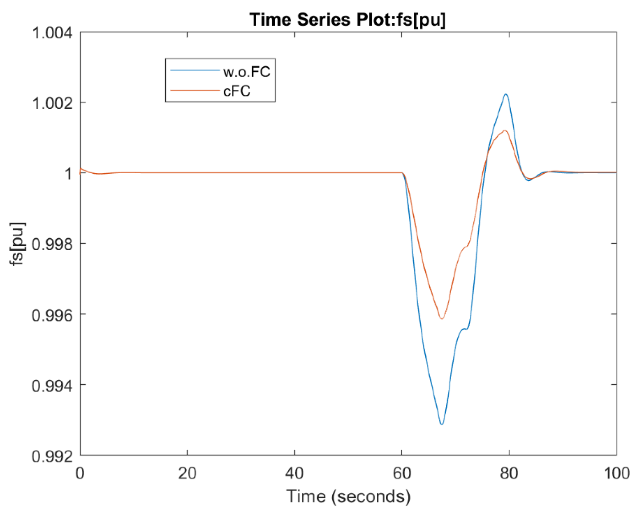
4.2. Small Sinusoidal Oscillations and Step down Load Active Power

In the previous case, before the perturbation, the reserve was entirely available to stabilize the frequency due to its load power constancy. This is far from the reality of a power system: the load continuously oscillates, entailing that a part of the reserve is already involved in the stabilization of the frequency. This means that if a sudden perturbation of the load power happens the system has less reserve available to face the variation.
The aim of this second type of simulations is to address how the continuous and small variability of the load affects the primary frequency control and its capability to face a step in load power, as well as to understand if the designed control for renewables is able to catch and follow these small load oscillations. The load power oscillations introduced in this simulation have an amplitude of 0.005 pu. The resulting frequency of Simulation 5 is presented in Figure 16.
It can be observed that the system with a complete FC needs some seconds to adapt to the sinusoidal variation of the load, but then it is able to follow it without problems. It is also possible to appreciate the huge reduction in the frequency nadir with respect to the base scenario, which is a fact that testifies one more time to the effectiveness of the updated control of the renewable generators. After the frequency peak, both systems are able to follow the sinusoidal oscillations of the load, but of course in the complete FC scenario the stabilization of the frequency is more evident and requires less time to be reached.
This simulation is particularly important for the validation of the innovative control of the renewables, since it is closer to the normal behavior of the load power.

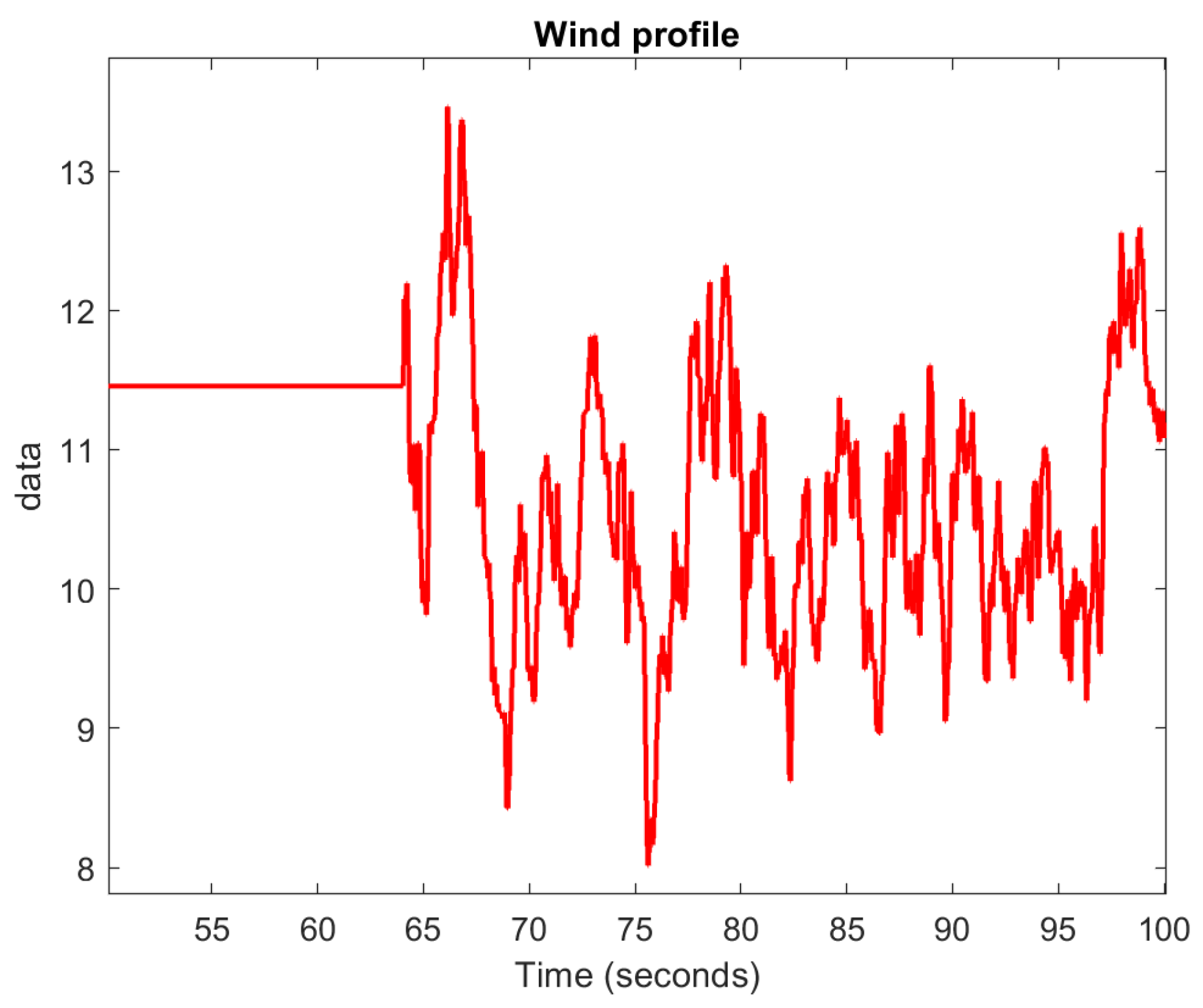
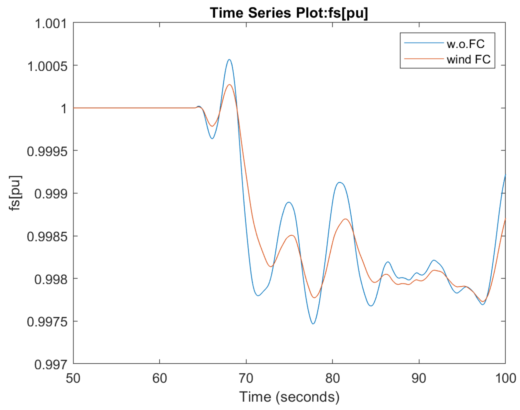
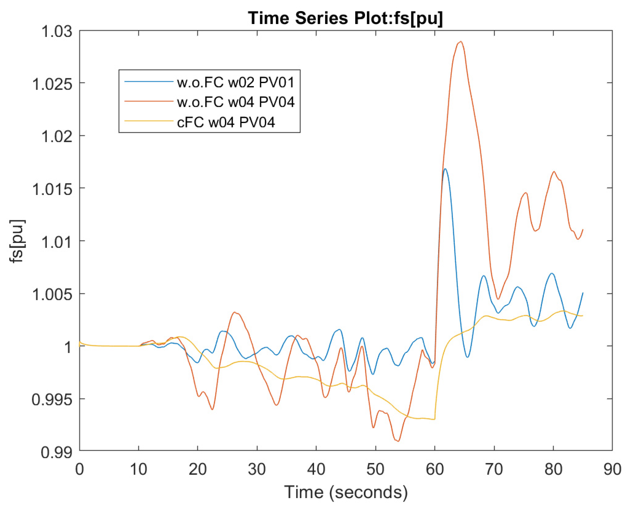
4.3. Variable Environmental Conditions

Two of the major drawbacks of renewables are the difficult predictability and the high variability of their primary resources, i.e., the wind and solar irradiance. In the field of primary frequency control, which takes place in the time window of a few seconds after a disturbance, this variability affects their response, especially for what concerns the wind energy. If the sun variations are fast but occur less frequently, the wind variations are huge and occur continuously. In this sense, the most critical situation is represented by windy days with some small clouds, in which both the wind and the irradiance are very variable.
The aim of these tests is to understand how much the variability of the renewable source affects primary frequency control if the renewables are rigid and they do not participate in it and, on the other hand, in the case they are able to modulate their power output to smooth their power variations. Furthermore, as for the second group, a part of the reserve will be already occupied to balance the natural variability of the resource, so, in case of a perturbation of the load, the reserve level could be less than the nominal amount.
The first analysis regards the most critical of the two resources: wind. In Simulation 6 and 7, the system is tested in the four scenarios with a real high variable wind profile. The wind profile has been downloaded from a DTU database of measurements in [38] and has the shape depicted in Figure 17.
The profile has been used as an input for the wind turbine system, which is not anymore free to adapt its output only to balance the frequency: now it also has to face a variable availability of the wind resource. This means that a part of the reserve could be already involved in the balancing of the frequency consequent to a wind speed variation, reducing the capability to counter a step of load power.
Simulation 6 studies the effect of the variable wind profile on the frequency. In particular, it is interesting to observe the response in the case of the wind turbine with virtual inertia control enabled compared with the base case without frequency response capabilities. The results are shown in Figure 18. In this simulation, the variability of the wind has been introduced after 64 s, so that its effects are more visible starting from a steady state condition.
In the base case without frequency control enabled, the wind turbines modulate their power to always produce at their maximum. This means that they do not detect that their behavior is causing the system’s frequency to oscillate. It is possible to observe, indeed, that the frequency has a number of peaks in correspondence with the peaks of the wind speed. This trend will stress the system, requiring an intense control action from the synchronous generators.
On the other hand, if the wind turbines are able to exploit their kinetic energy using the Extended OPPT method, it is evident how they smooth their power variation, producing lower peaks and stressing the power system less.
Looking at the largest nadir reached in the variable wind period, in the first scenario it is equal to 0.9975 pu (49.875 Hz), while in the updated scenario is 0.9977 pu (49.885 Hz). The reduction in the nadir is not so pronounced between the two, but the benefits consequent to the introduction of the Extended OPPT Method are evident considering the trend of frequency, since the amplitude of each oscillation is lowered. This fact is confirmed by the plot of the RoCoF, which highlights how the rate of variation of frequency is slower and smoother in the second scenario (Figure 19).
For what concerns the irradiance variation, Simulation 8 has been inspired by the dynamic EN50530 test, which is recognized as one of the techniques to evaluate the MPP tracking effectiveness [19]. It consists of a sequence of ramping up, constancy, and ramping-down the solar irradiance hitting the module. In this case, it has been adapted to model the shading of PV modules consequent to the passage of a small cloud. As can be seen in Figure 20, it consists of a steep ramping down (100 W/m2/s) from the nominal irradiance of 1000 W/m2 to 300 W/m2. Then, for few seconds, the irradiance remains low due to the shading and then it increases with the same steepness again to its nominal value.
The system with renewables participating in primary frequency control also shows variable irradiance to be more stable in terms of frequency, as depicted in Figure 21.

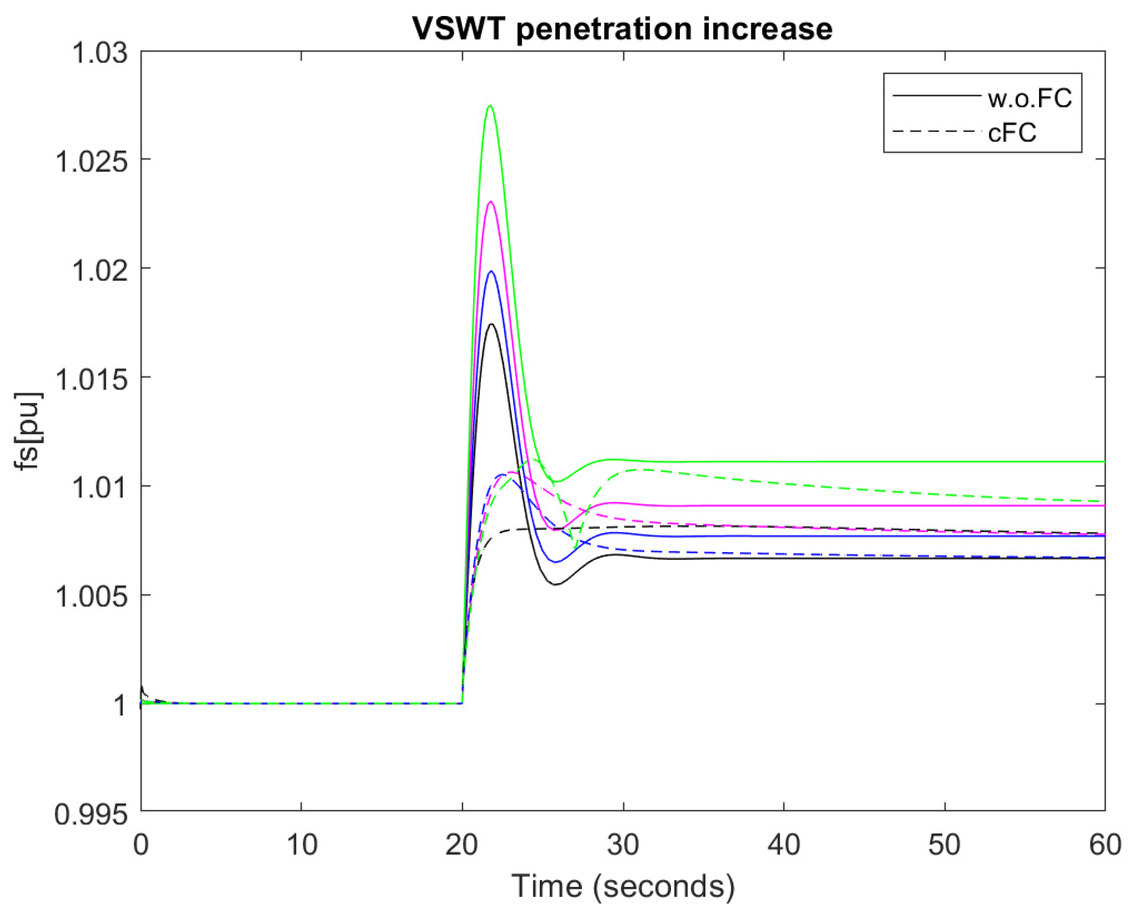
4.4. Increasing Renewables Penetration

The last scenario studied in this work is interesting in a long-term perspective. As explained in the introduction, in the future, a large spread of renewable sources is expected that will displace the conventional ones. In these simulations, the effect of such an increase on the frequency stability is addressed, both in the case of the absence of frequency response capability from renewables and in the presence of the advanced controls considered in this work.
It is important to remember the expected result of the tests in this first scenario: the increase in renewable penetration, due to their unpredictability and non-dispatchability, requires an increase in the reserve level, which at the same time displaces the conventional plants that are responsible for providing primary frequency controls and contributing to systems’ inertias. Due to these facts, the magnitude of the frequency nadir consequent to a perturbation is expected to increase as the penetration of renewables increases. The aim of the advanced controls, on the other hand, is to allow the substitution of the conventional fleet of generators with renewable ones without losing the ability to control the frequency. This is why, in the second case, a smaller frequency nadir and frequency oscillations are expected.
When adapting the participation factors, it is important to take into account that the displacement of synchronous generators causes a reduction in the system’s equivalent inertia. In this work, the reduction is proportional to the synchronous generator participation factor. This means, for example, that if the participation factor of the equivalent steam turbine passes from 0.7 to 0.35, the equivalent inertia constant will be halved.
The first group of simulations regards an increase in VSWT penetration, whose results are shown in Figure 22.
The solid lines represent the frequency variation consequent to a negative load power step of −10% in the scenario of primary frequency control provided just with synchronous generators, while the dashed lines are resulting from the scenario with a complete FC. Taking a first look at the plot, the negative effect of the increasing penetration of renewables if they are not able to participate in the primary frequency control is immediately clear. Indeed, for the same step of load power, the nadir increases from 1.0174 pu in the base case (20% wind, 10% PV) to 1.0275 pu in the most extreme case (50% wind, 10% PV). Furthermore, the difference in terms of the nadir between one curve and the other is not equal: increasing the wind penetration, the increase in the nadir is larger and larger from one curve to the next one. This happens because there is not just an effect due to the reduction in the synchronous generator power variation weight, but also of the system’s inertia.
Once stated thus, it can be seen how large the benefit is associated with the introduction of the frequency response capability in renewables: the nadir is much lower than in the first scenario and, as the penetration of VSWT increases, the mismatch between the two scenarios is way more evident. Unlike what happens in the first scenario, the nadir difference between the various curves in the second scenario reduces as the wind turbine penetration increases, meaning that the provision of this service from renewables (in this case, it prevails over the effect of the wind turbines inertial control since their weight is dominant) is able to “cover” the reduction in the system’s inertia, thus improving frequency stability.
The same kind of observations are discernable from the other simulations, which regard an increase in PV penetration (Figure 23).
In this case, the benefit is even larger, since, after a certain value of ppv, the nadir even reduces as the penetration of the photovoltaic increases. For example, in the most extreme case (40% PV, 20% wind), the nadir is lower than in the less PV-penetrated systems (10% PV, 20% PV, and 30% PV).
In a future scenario, it is not difficult to imagine power systems that are even largely penetrated by renewables. This case is studied in Simulation 17, with 80% of renewable participation. The correspondent results are shown in Figure 24.
It is evident that the benefit was obtained using the synergy between the Extended OPPT Method and the Power Reserve Control on the frequency stability. With such a renewable penetration, the system’s inertia is really small (−72% with respect to the base case) and, at the same time, a variation of power of the synchronous generator has just a small influence on the overall active power balance, accounting just for 20% of the per unit common basis power. The consequence of a drop in load power is potentially critical: a frequency nadir of 1.0446 pu corresponds to 52.23 Hz, which is an incredibly large frequency deviation.
On the other hand, the introduction of renewable updated controls and their coordination allows for a limiting of the nadir to 1.0082 pu (50.41 Hz), which is a perfectly acceptable value even facing an exceptionally strong perturbation event. By looking at the results of both simulations (11 and 15), in which, respectively, wind and PV penetration are equal to 40% as in Simulation 17, it can be observed that, if taken singularly, the frequency nadir is more accentuated, while in 17 the trend of the frequency is very flat. This fact enhances the idea that the two controls do not just act individually but that they support each other in the frequency control task due to their different response rates and they integrate very well with each other (Figure 25), obtaining a very smooth frequency trend and a satisfying frequency containment and stabilization.
Finally, it is very interesting to observe the effect of this control in a more dynamic situation. In particular, combining Simulation 7 (variable wind profile and load power step −10%) with Simulation 17 (40% wind, 40% PV), the frequency profile shown in Figure 26 is obtained.
It can be observed that the variability of the wind, as already demonstrated, has an increasing effect on the frequency instability if the penetration of the PV and wind turbine increases. If the system’s inertia decreases, indeed, the system frequency is more sensible to the perturbation, including the step introduced at time 60 s. In the case of an updated control of renewables, when they constitute the large majority of the generation fleet, it is evident how good they control the frequency in cases of variable wind profiles, smoothing almost all the peaks produced.

5. Conclusions and Future Developments Proposals

After the detailed analysis of the results of the simulations of the developed model shown in Section 4, it is possible to take stock of the work that has been carried out.
Looking ahead to a future in which renewables will be increasingly relevant in the energy mix, two strategies have been implemented to ensure they are able to help (or substitute) conventional generators in keeping the power system stable. In particular, Power Reserve Control and the Extended OPPT Method have been tested in this work, respectively, aiming at allowing photovoltaic modules and variable-speed wind turbines to participate in primary frequency control. Indeed, the challenge of using non-programmable renewable generators to provide the services that nowadays are delivered by fossil-fueled plants will become increasingly central, as the renewable presence increases to a more significant level.
In this sense, the results obtained in this work, especially when both controls coexist, are encouraging. Indeed, even if the Power Reserve Control introduces a very small increase in the RoCoF in the very few instants after a strong and sudden perturbation, the frequency nadir is reduced with respect to the case in which the frequency is not supported by renewables, especially in a future scenario in which they are massively present in the power system. The tradeoff between RoCoF increases and the nadir reduces in a given power system depending on its characteristics and, particularly, on the settings of the respective relays.
The model and the results rely on some simplifications, which generalize them but at the same time are lacking in detail. For this reason, there is an open field for future developments of the present work in some areas.
One of the possible fields of improvement is the modeling of the photovoltaic system, in particular for what concerns shading conditions and inequalities in sun resource distribution among the modules. Indeed, this would allow for a deeper study of the capability of photovoltaic systems in supporting the system’s frequency in more realistic situations.
Another possible improvement regards the modeling of the load. Indeed, it could be very interesting to better characterize its active power demand profile in case of a small island to cause the study to be even more realistic.
The last and more challenging proposal for future developments would be to model a small system node by node as the one studied in an overall way with the LFC approach in this work. This will completely fit it to a specific practical situation and ensure it is able to catch some details that are invisible with a general approach. At the same time, the adaptation to a very specific context removes one of the biggest advantages of the LFC approach, which is the generality and versatility of the developed model. Nevertheless, since the results obtained are promising, such improvements are interesting and can add cues to go deeper in the knowledge of this field.

Author Contributions

Conceptualization, S.M.; methodology, S.M.; software, L.R.; validation, L.R. and S.M.; formal analysis, L.R. and S.M.; investigation, L.R. and S.M.; resources, L.R. and S.M.; data curation, L.R.; writing—original draft preparation, L.R.; writing—review and editing, S.M.; visualization, L.R.; supervision, S.M.; project administration, S.M.; funding acquisition, S.M. All authors have read and agreed to the published version of the manuscript.

Funding

This research was funded by the Spanish national research agency Agencia Estatal de Investigación, grant number PID2019-108966RB-I00/AEI/10.13039/501100011033.

Institutional Review Board Statement

Not applicable.

Informed Consent Statement

Not applicable.

Data Availability Statement

Not applicable.

Conflicts of Interest

The authors declare no conflict of interest. The funders had no role in the design of the study; in the collection, analyses, or interpretation of data; in the writing of the manuscript; or in the decision to publish the results.

Appendix A. Values of Constants Used in the Model
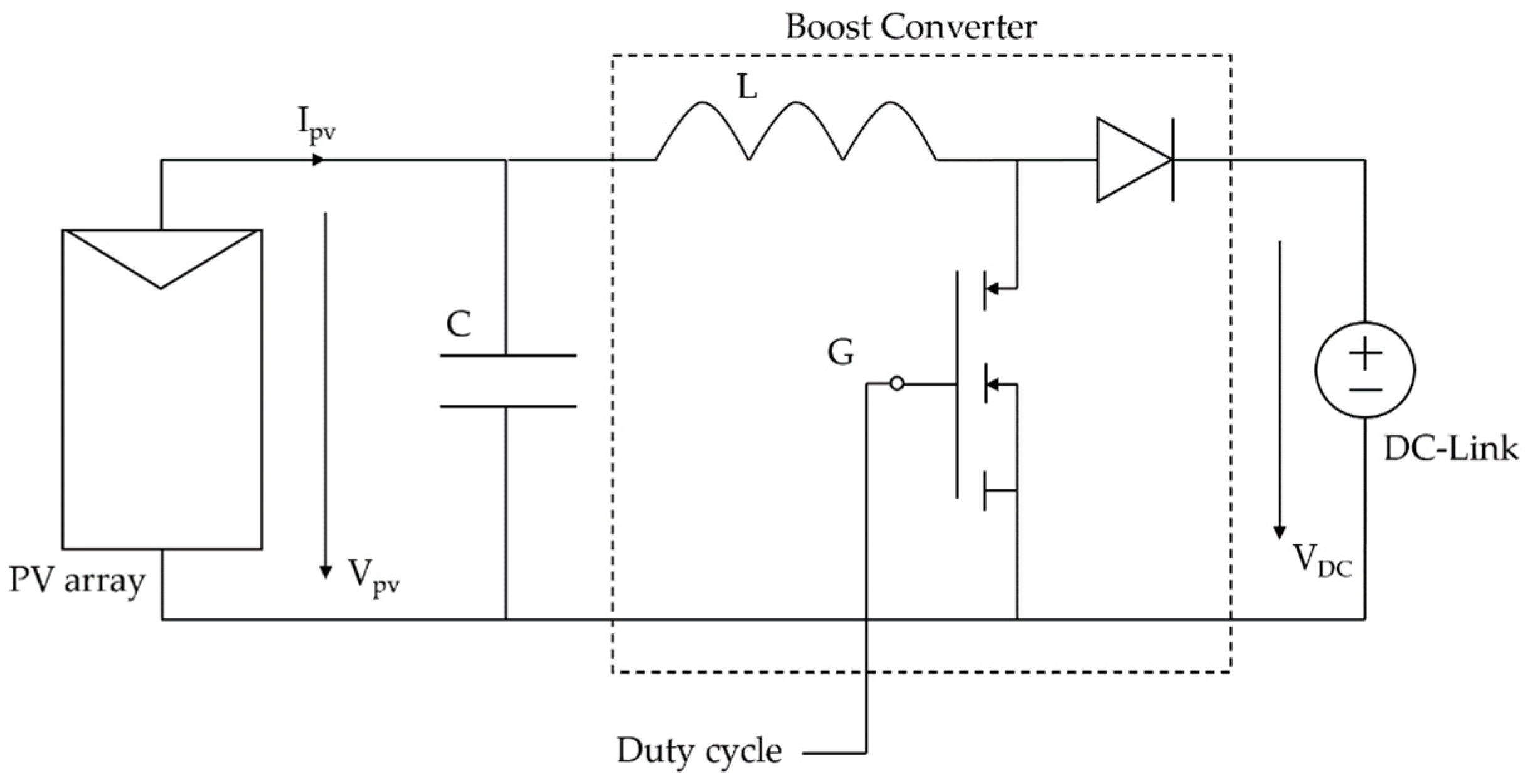
This appendix compiles the values of the constants used in the model, organized as a function of the subsystems in which they are located.
  • PV subsystem
    PV module: Solartech Power SPM210P (four modules in series and variable number of arrays as a function of the participation factors)
    Ccapacitor = 100 μF
    Linductor = 10 mH
    D-controlled boost converter with default Simulink settings
    PI controller: P = 0.03; I = 1
    Droop constant of active power reserve adaptation = 0.05
    Initial reserve level = 0.2
  • VSWT system
    Pbase = Pt,base = Pg,base = 1.5 MW, vnom = 12 m/s, ωt,base = 1.644 rad/s, ωg,base = 157.08 rad/s, f = 50 Hz
    Values for the model blocks taken from [36]
    Speed governor PI controller: P = 3; I = 80
    Pitch governor P controller: P = 500
    Inertial control [24,39]: Kopt = 0.4225, kvir = 8, Wvir = 0.2, Two = 10 s, Tlp = 100 ms, HWT = 5.29 s
  • Steam turbine with one reheat [24,32]
    Heq = 2.88 s
    Droop constant = 0.05
    τg = 0.2
    FHP = 0.3
    TRH = 5 s
    TCH = 0.3 s

References

  1. European Council. Available online: https://www.consilium.europa.eu/en/policies/climate-change/paris-agreement/ (accessed on 1 August 2022).
  2. UNFCCC. Available online: https://unfccc.int/process-and-meetings/the-paris-agreement/the-paris-agreement (accessed on 1 August 2022).
  3. IEA. Available online: https://www.iea.org/data-and-statistics/data-browser?country=WORLD&fuel=CO2%20emissions&indicator=CO2BySector (accessed on 2 August 2022).
  4. European Energy Agency. Available online: https://www.eea.europa.eu/ims/share-of-energy-consumption-from (accessed on 2 August 2022).
  5. IRENA. Global Energy Transformation—A Roadmap to 2050; International Renewable Energy Agency: Abu Dhabi, United Arab Emirates, 2019. [Google Scholar]
  6. IRENA. Grid Codes for Renewable Powered Systems; International Renewable Energy Agency: Abu Dhabi, United Arab Emirates, 2022. [Google Scholar]
  7. Hassan, F.; Bollen, M. Integration of the Distributed Generation in the Power System; IEEE Press: New York, NY, USA, 2011. [Google Scholar]
  8. Riquelme-Dominguez, J.M.; De Paula Garcia-Lopez, F.; Martínez, S. Power Ramp-Rate Control via power regulation for storageless grid-connected photovoltaic systems. Int. J. Electr. Power Energy Syst. 2022, 138, 107848. [Google Scholar] [CrossRef]
  9. Brivio, C.; Mandelli, S.; Merlo, M. Battery energy storage system for primary control reserve and energy arbitrage. Sustain. Energy Grids Netw. 2016, 6, 152–165. [Google Scholar] [CrossRef]
  10. NREL. On the Path to Sunshot: The Role of Advancements in Solar Photovoltaic Efficiency, Reliability, and Costs; NREL: Golden, CO, USA, 2016.
  11. Solomon, A.A.; Bogdanov, D.; Breyer, C. Curtailment-storage-penetration nexus in the energy transition. Appl. Energy 2019, 235, 1351–1368. [Google Scholar] [CrossRef]
  12. Sangwongwanich, A.; Yang, Y.; Blaabjerg, F. Development of Flexible Active Power Control Strategies for Grid-Connected Photovoltaic Inverters by Modifying MPPT Algorithms. In Proceedings of the 2017 IEEE 3rd International Future Energy Electronics Conference and ECCE Asia, Kaohsiung, Taiwan, 3–7 June 2017. [Google Scholar]
  13. Batzelis, E.I.; Kampitsis, G.E.; Papathanassiou, S.A. Power Reserves Control for PV Systems With Real-Time MPP Estimation via Curve Fitting. IEEE Trans. Sustain. Energy 2017, 8, 1269–1280. [Google Scholar] [CrossRef]
  14. Sangwongwanich, A.; Yang, Y.; Blaabjerg, F.; Sera, D. Delta Power Control Strategy for Multi-String Grid-Connected PV Inverters. IEEE Trans. Ind. Appl. 2017, 53, 3862–3870. [Google Scholar] [CrossRef] [Green Version]
  15. Li, X.; Wen, H.; Zhu, Y.; Jiang, L.; Hu, J.; Xiao, W. A Novel Sensorless Photovoltaic Power Reserve Control With Simple Real-Time MPP Estimation. IEEE Trans. Power Electron. 2019, 34, 7521–7531. [Google Scholar] [CrossRef]
  16. Hoke, A.; Chakraborty, S.; Shirazi, M.; Muljadi, E. Rapid Active Power Control of Photovoltaic Systems for Grid Frequency Support. IEEE J. Emerg. Sel. Top. Power Electron. 2017, 5, 1154–1163. [Google Scholar] [CrossRef]
  17. Riquelme-Dominguez, J.M.; Martinez, S. A Photovoltaic Power Curtailment Method for Operation on Both Sides of the Power-Voltage Curve. Energies 2020, 13, 3906. [Google Scholar] [CrossRef]
  18. Nanou, S.; Papakonstantinou, A.; Papathanassiou, S. A generic model of two-stage grid-connected PV systems with primary frequency response and inertia emulation. Electr. Power Syst. Res. 2015, 127, 186–196. [Google Scholar] [CrossRef]
  19. Riquelme-Dominguez, J.M.; Martínez, S. Systematic Evaluation of Photovoltaic MPPT Algorithms Using State-Space Models Under Different Dynamic Test Procedures. IEEE Access 2022, 10, 45772–45783. [Google Scholar] [CrossRef]
  20. Aziz, A.; Oo, A.T.; Stojcevski, A. Frequency regulation capabilities in wind power plant. Sustain. Energy Technol. Assess. 2018, 26, 47–76. [Google Scholar] [CrossRef]
  21. Clark, K.; Miller, N.W.; Sanchez-Gasca, J.J. Modelling of GE Wind Turbine-Generators; Tech. Rep.; Version 4.5; General Electric International: Schenectady, NY, USA, 2010. [Google Scholar]
  22. Engelken, S.; Mendonca, A.; Fischer, M. Inertial response with improved variable recovery behaviour provided by type 4 WTs. IET Renew. Power Gener. Spec. 2017, 11, 195–201. [Google Scholar] [CrossRef]
  23. Wu, Y.; Shu, W.; Hsieh, T.; Lee, T. Review of inertial control methods for DFIG-based wind turbines. Int. J. Electr. Energy 2015, 3, 174–178. [Google Scholar] [CrossRef] [Green Version]
  24. Ochoa, D.; Martínez, S. Analytical Approach to Understanding the Effects of Implementing Fast-Frequency Response by Wind Turbines on the Short-Term Operation of Power Systems. Energies 2021, 14, 3660. [Google Scholar] [CrossRef]
  25. Vidyanandan, K.V.; Senroy, N. Primary frequency regulation by deloaded wind turbines using variable droop. IEEE Trans. Power Syst. 2013, 28, 837–846. [Google Scholar] [CrossRef]
  26. Hwang, M.; Muljadi, E.; Park, J.W.; Sorensen, P.; Kang, T.C. Dynamic droop-based inertial control of a doubly-fed induction generator. IEEE Trans. Sustain. Energy 2016, 7, 924–933. [Google Scholar] [CrossRef]
  27. Fairley, P. Can Synthetic Inertia from Wind Power Stabilize Grids? IEEE Spectrum 2016, 7. [Google Scholar]
  28. Fu, Y.; Zhang, X.; Hei, Y.; Wang, H. Active participation of variable speed wind turbine in inertial and primary frequency regulations. Electr. Power Syst. Res. 2017, 147, 174–184. [Google Scholar] [CrossRef]
  29. Martínez-Lucas, G.; Sarasua, J.I.; Perez-Diaz, J.I.; Martínez, S.; Ochoa, D. Analysis of the Implementation of the Primary and/or Inertial Frequency Control in Variable Speed Wind Turbines in an Isolated Power System with High Renewable Penetration. Case Study: El Hierro Power System. Electronics 2020, 9, 901. [Google Scholar] [CrossRef]
  30. Díaz-González, F.; Hau, M.; Sumper, A.; Bellmunt, O. Participation of wind power plants in system frequency control: Review of grid code requirements and control methods. Renew. Sustain. Energy Rev. 2014, 34, 551–564. [Google Scholar] [CrossRef]
  31. O’Sullivan, J.; Rogers, A.; Flynn, D.; Smith, P.; Mullane, A.; O’Malley, M. Studying the maximum instantaneous non-synchronous generation in an island system—Frequency stability challenges in Ireland. IEEE Trans. Power Syst. 2014, 29, 2943–2951. [Google Scholar] [CrossRef]
  32. Kundur, P. Power System Stability and Control; Electric Power Research Institute: Palo Alto, CA, USA, 1993. [Google Scholar]
  33. Li, S.; Deng, C.; Shu, Z.; Huang, W.; Jun He, J.; You, Z. Equivalent inertial time constant of doubly fed induction generator considering synthetic inertial control. J. Renew. Sustain. Energy 2016, 8, 053304. [Google Scholar] [CrossRef]
  34. Ibrahim, H.; Anani, N. Variations of PV module parameters with irradiance and temperature. Energy Procedia 2017, 134, 276–285. [Google Scholar] [CrossRef]
  35. Carrero, C.; Ramírez, D.; Rodríguez, J.; Platero, C.A. Accurate and fast convergence method for parameter estimation of PV generators based on three main points of the I-V curve. Renew. Energy 2011, 36, 2972–2977. [Google Scholar] [CrossRef]
  36. Ochoa, D.; Martínez, S. A Simplified Electro-Mechanical Model of a DFIG-based Wind Turbine for Primary Frequency Control Studies. IEEE Lat. Am. Trans. 2016, 14, 3614–3620. [Google Scholar] [CrossRef] [Green Version]
  37. Eto, J.H. Use of Frequency Response Metrics to Assess the Planning and Operating Requirements for Reliable Integration of Variable Renewable Generation; Lawrence Berkeley National Laboratory: Berkeley, CA, USA, 2011; Available online: https://escholarship.org/uc/item/0kt109pn (accessed on 20 October 2022).
  38. DTU Data: Database on Wind Characteristics. Available online: https://gitlab.windenergy.dtu.dk/fair-data/winddata-revamp/winddata-documentation/-/blob/master/readme.md/ (accessed on 20 October 2022).
  39. Ochoa, D.; Martinez, S. Fast-Frequency Response Provided by DFIG-Wind Turbines and Its Impact on the Grid. IEEE Trans. Power Syst. 2017, 32, 4002–4011. [Google Scholar] [CrossRef]
Figure 1. Power-voltage curve of a PV module for two different ambient conditions, showing the maximum power point (MPP) and the possible reference operating points for a 20% reserve.
Applsci 12 11126 g001
Figure 2. Single-stage grid-connected PV system.
Applsci 12 11126 g002
Figure 3. Active power frequency control research lines in wind-based power plants.
Applsci 12 11126 g003
Figure 4. General layout of the model.
Applsci 12 11126 g004
Figure 5. Photovoltaic system model: (a) General flowchart showing the electrical model (left block) and the voltage control (right block); (b) Simulink implementation, including the electrical model (upper subsystem) and the voltage control (bottom subsystem).
Applsci 12 11126 g005
Figure 6. Voltage control subsystem: (a) General flowchart; (b) Simulink implementation.
Applsci 12 11126 g006
Figure 7. PV electrical subsystem diagram.
Applsci 12 11126 g007
Figure 8. Block diagram of a VSWT model.
Applsci 12 11126 g008
Figure 9. Extended OPPT Method [24].
Applsci 12 11126 g009
Figure 10. Simulation 1 frequency trend.
Applsci 12 11126 g010
Figure 11. Simulation 1 RoCoF.
Applsci 12 11126 g011
Figure 12. Simulation 2 frequency trend.
Applsci 12 11126 g012
Figure 13. Simulation 3 frequency trend.
Applsci 12 11126 g013
Figure 14. Simulation 4 frequency trend.
Applsci 12 11126 g014
Figure 15. Generator power variations in Simulation 4.
Applsci 12 11126 g015
Figure 16. Simulation 5 frequency trend.
Applsci 12 11126 g016
Figure 17. Real wind profile used in the simulations.
Applsci 12 11126 g017
Figure 18. Simulation 6 frequency trend.
Applsci 12 11126 g018
Figure 19. Simulation 6 RoCoF.
Applsci 12 11126 g019
Figure 20. Simulation 8 irradiance profile.
Applsci 12 11126 g020
Figure 21. Simulation 8 frequency trend.
Applsci 12 11126 g021
Figure 22. VSWT penetration increase.
Applsci 12 11126 g022
Figure 23. PV penetration increase.
Applsci 12 11126 g023
Figure 24. Simulation 17 frequency trend.
Applsci 12 11126 g024
Figure 25. Simulation 18 power variations.
Applsci 12 11126 g025
Figure 26. Simulation 7 for different scenarios frequency trend.
Applsci 12 11126 g026
Table 1. Summary of reviewed articles about Power Reserve Control of PV systems.
AuthorsReference
1Batzelis et al.[13]
2Sangwongwanich et al.[14]
3Li et al.[15]
4Hoke et al.[16]
5Riquelme et al.[17]
Table 2. Simulation groups and aims.
Simulation GroupAim
Load active power step up/downObserving the frequency response of the system after a sudden variation of the load power for different step magnitudes
Small sinusoidal oscillations + step of load active powerObserving the frequency response of the system to small and continuous variations of the load, i.e., similar to the real behavior, and to a step if a part of the reserve is already in use to balance the small variations
Variable environmental conditions (real wind speed profile, irradiance variations)Understanding how the system responds to environmental condition changes, as well as to a sudden load power variation in such a situation
Variable participation factorsUnderstanding what is the impact of an increasing penetration of renewable sources on the system’s frequency stability
Table 3. Summary of Simulation 1–8.
N° SimulationFeatures
1Step up Pload +1%
2Step down Pload −1%
3Step down Pload −2%
4Step down Pload −10%
5Small sinusoidal variation of Pload (amplitude 5‰) + step down Pload −10%
6Real wind profile
7Real wind profile + step down Pload −10%
8Steep irradiance ramp up—ramp down
Table 4. Summary of Simulation 9–17.
N° Simulationpwindpsynchronousppv
90.30.60.1
100.40.50.1
110.50.40.1
120.20.60.2
130.20.50.3
140.20.40.4
150.30.50.2
160.40.30.3
170.40.20.4
Publisher’s Note: MDPI stays neutral with regard to jurisdictional claims in published maps and institutional affiliations.

