Abstract
The proposed model of the neural network (NN) describes the optimization task of the water meter body assembly process, based on 18 selected production parameters. The aim of this network was to obtain a certain value of radial runout after the assembly. The tolerance field for this parameter is 0.2 mm. The repeatability of this value is difficult to achieve during production. To find the most effective networks, 1000 of their models were made (using various training methods). Ten NN with lowest errors of the output value prediction were chosen for further analysis. During model validation the best network achieved the efficiency of 93%, and the sum of squared residuals (SSR) was 0.007. The example of the prediction of the value of radial runout of machine parts presented in this paper confirms the adopted statement about the usefulness of the presented method for industrial conditions and is based on the analysis of hundreds of thousands of parametric and descriptive data on the process flow collected to create an effective network model.
1. Introduction
Most artificial neural network models base their operation on highly simplified brain dynamics, although they increasingly reflect more real-life biological models. They are also increasingly used as computational tools to solve complex pattern recognition, function estimation and classification problems. Neutral networks can also be a solution to highly complex and multi-criteria problems related to various types of production processes, including assembly, machining and manufacturing processes.
Examples of this type of solution are presented, inter alia, in [1], where the application of the neural network to additive manufacturing is presented. This paper overviews the progress of applying the neural networks algorithm to several aspects of the additive manufacturing, including model design, quality evaluation and current challenges, in applying NN in this field. The problem of applying NN in additive manufacturing.
It has also been recently discussed in [2], where an example of the detection of processing defects in laser powder bed fusion additive manufacturing is presented. A convolutional neural network (CNN) was used in this case for autonomous detection and classification of many spreading anomalies. It is important that the input layer of the CNN is modified to enable the algorithm to learn both the appearance of the powder bed anomalies and contextual information at multiple size scales. This change increases the flexibility and classification accuracy of the algorithm. The use of neural networks in manufacturing process can also be found in many other works, such as in [3], where the problem of the optimization of milling operations using artificial neural networks (ANN) and simulated annealing algorithm (SAA) is discussed, or in [4], describing the optimization of the manufacturing process parameters using deep neural networks as surrogate models.
The considerations presented in this article concern an example of the application and selection of a neural network on the example of a specific production process. By building a model on a real working process, which will allow the network to be improved over time as the network is trained, an example of a highly useful working solution has been obtained, functioning in one of the largest water meters manufacturing companies in Europe. The article is, therefore, an example of applied science in industry, and its basis was the collection of hundreds of thousands of data, describing the process and parameters of products. The presented solution refers to the technological process of production, i.e., hot forging, machining and assembly of parts used to produce a device for measuring drinking water consumption. The quality requirements for this type of products put a strong emphasis on the final dimensional characteristics along with deviations in shape and position for the manufactured object after assembly operations. This has a critical impact on its further functioning in the operation/operational conditions. Low tolerance range for selected essential characteristics is a result of product legalization periods determined by the law and the strictly defined parameters of the accuracy of drinking water consumption measurements, which is important, among others, due to the care for the natural environment. One of those essential characteristics is the radial runout of the axle mounted in the hole in the bottom of the body. It is determined in relation to one of its internal diameters, which is influenced by the appropriate performance of not only assembly operations, but also technological operations preceding the assembly itself, which was the subject of this study.
In the analyzed case, the field of radial runout tolerance (Figure 1) after assembly is 0.2 mm, which is a value that is difficult to achieve repeatedly in production.

Figure 1.
Determination of the radial runout after the assembly process.
Construction of the assembly line and its elements is shown in detail in Figure 2.
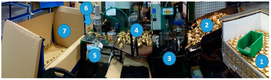
Figure 2.
Assembly line for water meter bodies with elements: 1—Storage bay with a basket of processed water meter bodies intended for assembly components, 2—Auxiliary tray for machined bodies, 3—Station for assembling the strainer and damming plate in the water meter body, 4—Transitional storage bay for partially assembled bodies, 5—Station for mounting the axle in the water meter body, 6—Control of the depth of the axle seating in the water meter body, 7—Storage bay with a basket for the assembled water meter bodies.
The machined water meter bodies are delivered to the storage area 1 in metal baskets, organized in layers separated with cardboard dividers, ready for component assembly. Elements are already washed, purged and dried. The auxiliary tray 2 serves as a buffer storage for mounting the water meter bodies in station 3, where a worker assembles the strainer and damming plate. Station 3 consists of a pneumatic actuator and the device for facing a damming plate, which is in fully configurable in terms of damming plate type, damming plate mounting angle and the size of the thread on the inlet port. The working element of the press at station 3 is a TOX Q-S 015.030.100.12 actuator and an actuator—spring presser, which ensures optimal constipation of the body in the time of satiating. On the transit storage bay 4, the employee operating the station 3 places partially assembled pieces for an employee operating at the axle setting station 5. The employee operating the station 5 takes the appropriate basic axle from the box and seat it with the correct side in the tool hole. After embedding the axle, the body is taken from the field of the transition bay 4 and located on the punching device, then the work is done by the EMG 6PHR press. After embedding the axle in the water meter body, an employee from station 5 checks 100% of the pieces of 8.1 mm + 0.1 mm of axle seating on the control device 6. After the final inspection, the worker from station 5 packs the assembled body into a metal basket located in the storage field 7.
2. Materials and Methods
2.1. Artificial Neural Networks in Mechanical Assembly Problem
Due to the fact that designing and optimizing the technological process of assembly is a very complex, multi-criteria issue [5,6,7], various heuristic techniques are used for these problems, resulting in finding approximately optimal solutions, due to specific criteria. This problem in most cases concerns ASP (assembly sequence planning) problem and can be solved, for example, by selected heuristics. In research on ASP, very different heuristic optimization algorithms were used, such as the genetic algorithm (GA) [8,9,10] or artificial neural networks (ANN), that are the main subjects of this article [11,12,13].
In [14] the authors came up with a three-step integrated solution with some heuristic working rules to help generate an efficient sequence of assembly. In the mentioned paper, the use of a backpropagated neural network for optimization of the assembly sequence is presented. The outcome showed that the introduced model can enable the optimization of the assembly sequence and allows the designer to perceive the contact relationship and assembly limitation of the three-dimensional elements.
Attempts to use ANN in mechanical assembly can also be found in other applications. The paper [15] presents the application of the method of artificial neural networks to detect faulty assembly processes with the use of wearable technology. The paper deals with the problem of distinguishing between correct and faulty operations in assembly tasks. A digital assembly glove was used for this purpose. To classify the signal from the glove, artificial neural network methodology was used. The network performance was tested in the selected assembly process.
In the paper [16], authors presented system for assembly parts recognition, applying convolutional neural networks. Deep neural networks have been used to identify and recognize mounting parts (bolts, nuts) and mounting features (holes) to speed up any augmented reality mounting process.
The article [17] presents the use of component models instead of the entire assembly model for predicting assembly quality defects during the production of automotive equipment. For this purpose, artificial neural networks were used to predict assembly time and market value based on assembly models.
Artificial neural networks and also machine learning [18,19,20,21,22] are, thus, information processing paradigms inspired by the natural biological nervous system. The decision network consists of a large number of highly interconnected processing elements (neurons) that perform some basic operations on their input to solve a specific problem. The neurons that make up the network are linked together by synapses. Synapses have assigned weights, i.e., numerical values, the interpretation of which depends on the model (in the studied case the model of technological assembly process).
The input vector is multiplied by the synaptic weights vector. This operation performs a function of the postsynaptic potential and allows one to determine the value of the signal calculated on the basis of the sum of input signals multiplied by synaptic weights.
Artificial neuron models can be interpreted as mathematical models. W. McCullach and W. Pitts in 1943 proposed the model of biological neurons, which is considered to be the first model of a neural network, with a given relationship:
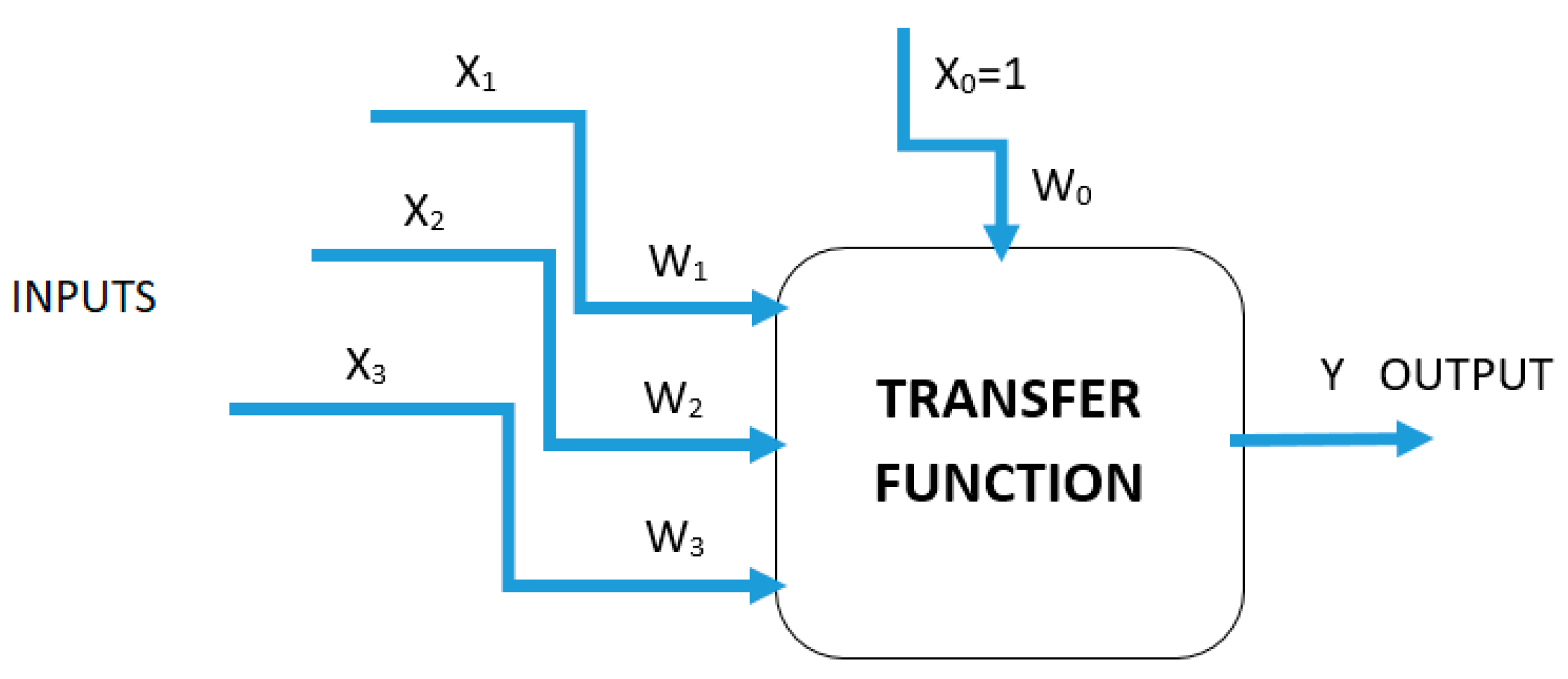
The typical signal route between neurons (processing units) is presented in Figure 3, where xi are the input signals of the neurons (or external input data for system), wi are the weights of the edge connections (synapses), w0 is the sensitivity threshold of the neuron (the so-called bias), and f (·) is a simple non-linear function, for example, a sigmoid or a logistic function. Activation (transfer) functions (AF) are possible for each hidden and output layer.
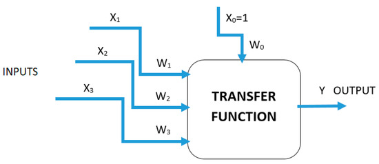
Figure 3.
Symbolic representation of the neuron’s model.
In this study logistic, exponential, linear, sine and tanh functions were tested, which were used to activate hidden and output layers. To activate a neuron, the sum of each signal multiplied by the corresponding weight has to be equal to or greater than the sensitivity threshold w0, otherwise it remains inactive. An input signal can be an excitatory or inhibitory type, depending on the positive or negative sign of the weight value [23].
2.2. The Concept of a System Supporting the Optimization of Radial Runout in the Assembly Process Based on Artificial Neutral Networks
The presented tool, using ANN, aims to predict, due to the selected criteria, the magnitude of the radial runout parameter for a selected case in a production plant. During the assembly process of the water meter, the following parameters are taken into account:
- The value of the clamping force for the first and second assembly steps;
- Number of cycles performed by presser (it is possible to replace it);
- Time of applied force in the second assembly operation;
- The type of used clamp;
- Sequence of assembly procedures.
The selection of the presented criteria was preceded by a long-term analysis and testing of many other criteria.
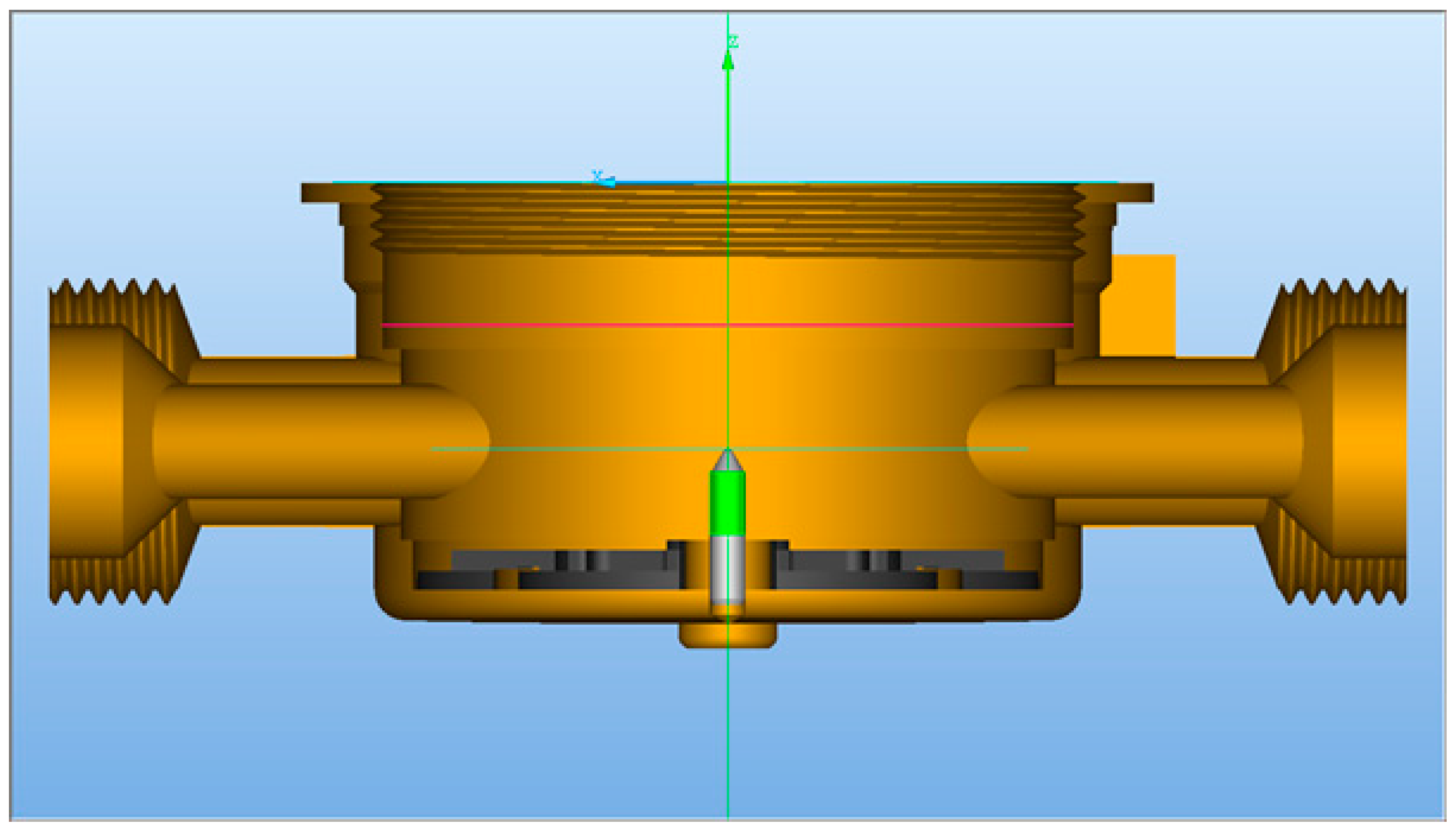
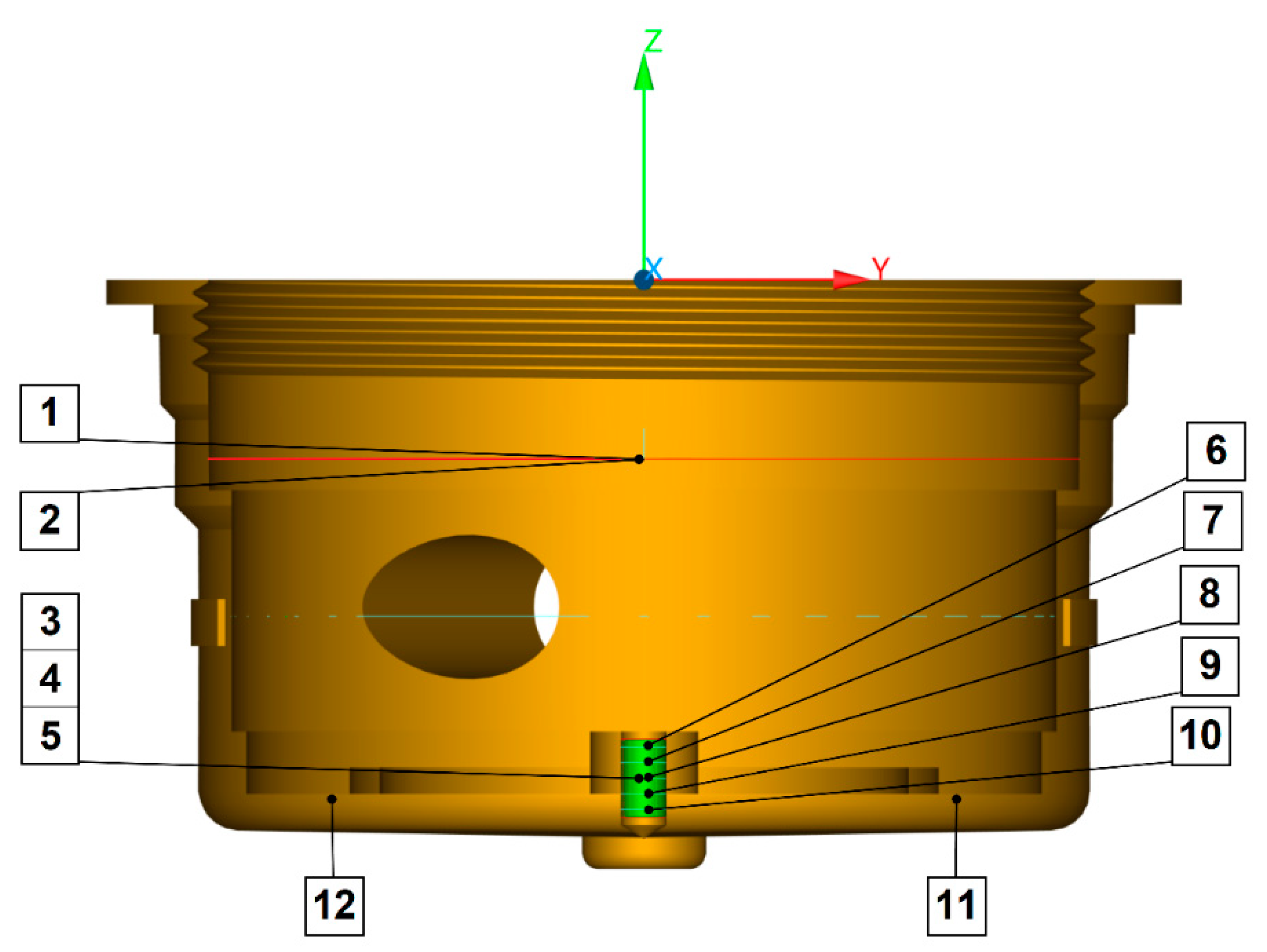
It was assumed that the hot-forged body with specific dimensional characteristics is delivered for assembly (the forging process also takes place in the discussed plant). Parameters and input characteristics that may have a significant impact on the final result of the radial runout value were determined. As a result, after hot forging and machining operations, the following parameters were measured (Figure 4).

Figure 4.
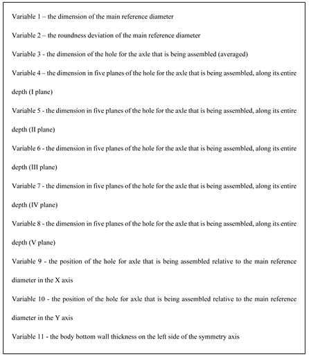
Parameters and input characteristics: 1—the dimension of the main reference diameter, 2—the roundness deviation of the main reference diameter, 3—the dimension of the hole for the axle that is being assembled (averaged), 4—the position of the hole for axle that is being assembled relative to the main reference diameter in the X axis, 5—the position of the hole for axle that is being assembled relative to the main reference diameter in the Y axis, 6, 7, 8, 9, 10—the dimension in five planes of the hole for the axle that is being assembled, along its entire depth, 11, 12—the body bottom wall thickness on the left and right sides of the symmetry axis.
- The dimension of the main reference diameter;
- The roundness deviation of the main reference diameter;
- The dimension of the hole for the axle that is being assembled (averaged);
- The dimension in five planes of the hole for the axle that is being assembled, along its entire depth;
- The position of the hole for axle that is being assembled relative to the main reference diameter in the X axis;
- The position of the hole for axle that is being assembled relative to the main reference diameter in the Y axis;
- The body bottom wall thickness on the left and right sides of the symmetry axis;
- The average thickness of the body bottom.
The measurements were carried out using the LH65 coordinate measuring machine by WENZEL with a measurement uncertainty MPEp of 1.5 μm. The dimensions of the measured bodies were recorded by a Renishaw PH20 5-axis touch-trigger system with a ruby stylus. To determine the dimension of the main reference diameter, a circle was measured at 12 measurement points. The hole diameters in five planes were obtained by measuring 5 points on the circle in each of the 5 cross-section planes. Measurements were made for 4000 bodies.
2.3. Assumptions of a Neural Network
The goal of ANN was to assess the influence of particular parameters of the assembly process on the magnitude of axle radial runout in the water meter body. The first step was to prepare the training set, which consisted of the input and output data. Previously presented dimensional characteristics of the body and selected parameters of the assembly process served as the input data.
After preparing the set of training data, the individual numerical values were normalized to obtain independence between them and at the same time to ensure their equivalence. To normalize initial variables, which values were in different ranges, linear transformation was used. This approach allowed us to represent each variable in a range between 0 and 1. Data were normalized using the rescaling function, dividing the difference between the original and minimal values, by the range of data set, according to the equation:
Quantitative variables were converted according to the min–max function to numbers in the range 0–1. Qualitative variables were assigned values of 0, when the feature was not obtained, and values of 1, otherwise.
Training the neural network in order to obtain the appropriate efficiency is based on minimizing the prediction error function, defined by the sum of squared residuals (SSR), described as follows:
where: n—number of training examples, yi—expected network output value, yi*—measured network output value.
Mentioned error function calculates the divergence between the network output values and the a priori output values form teaching set of data. The error surface has paraboloid shape with one distinct minimum. The network error is calculated iteratively after each repetition of training algorithm—epoch. Based on its value, it is possible to assess and modify only those weights that are associated with neurons in the last layer. Weights of signals in remaining layers can be trained by using backpropagation algorithm. In this approach each neuron has an assigned error value, calculated based on the error value of all those neurons, to which it sends its output value. The backpropagation algorithm is applied in the reverse direction from normal data flow, i.e., from output to input.
The efficiency of a neural network is defined as the ratio of correctly approximated or classified cases to all cases included in the data set.
Network performance can be influenced by following parameters: the number of hidden layers, number of neurons in each layer, existence of an additional neuron—bias, network learning rules, including the learning algorithm and activation function. Mentioned parameters were empirically selected to achieve the best prediction efficiency.
Each set of process data, prepared for passing to the network has to be divided into three groups:
(1) A sequence of training data, selected to allow the mapping of the considered prediction task;
(2) Test data checking the network operation, including the assessment of changes made during subsequent learning cycles;
(3) Verification data evaluating network efficiency based on the set of data, which was not used before.
The data were divided into three groups: teaching (70%), testing (15%) and validation (15%). The division of datasets into each of these groups was done using K-Fold cross validation. Size and number of hidden layers are set empirically, training the network multiple times. This approach allows us to find balance between its overgrown structure and performance. The output layer of the ANN is a set of neurons, determining output signals. The number of neurons in the output layer is identical to the number of output data constituting the result of the network. The number of neuron inputs is related to the number of signals that are either the fed to the network or are output signals from preceding layer. Moreover, in the model of the neuron there may exist additional, independent signal inputs, with constant value +1. This signal, same as the rest of the signals, is scaled by its own weight, which is calculated during training process. The neural network consists of three layers: input (18 neurons), output (1 neuron) and one hidden (3 neurons). The network architecture, mainly the size of the hidden layer, was selected empirically, taking into account the accuracy of the results prediction.
Performance of the ANN is highly affected by selection of activation functions. Those functions, based on the sum of weighted signals, set neuron’s output. The most common activation functions are: linear, where argument is passed directly to the output; logistic (S-shaped curve with output range from 0 to 1); hyperbolic (with output values within the range of −1 to 1); and exponential.
Selecting the correct ANN learning algorithm has a crucial impact on the network performance. Learning algorithm iteratively changes the weights assigned to neurons inputs, trying to minimize the output error calculated in each iteration, based on the data set, which were fed to the network.
In this paper, from a variety of ANN learning techniques, the main focus was put on the method of the steepest descent (SD), the BFGS (Broyden–Fletcher–Golfarb–Shanno) method and the conjugate gradient method (CG).
The steepest descent method is a modification of the simple gradient descent method. Both methods are iterative optimization algorithms used to find extremum of the function. In contrast to the simple gradient descent method, where search direction proceeds with constant arbitrary selected step size, in the SD method, step size can vary, to ensure the biggest decrease in the value of the function at the new point. Characteristic feature in SD method in each search direction is orthogonal to the one from previous iterations.
Implementation of SD requires significant number of searches, which is resource intensive and time consuming.
Mentioned issues can be overcome using conjugate directions method. The goal of that algorithm is to determine the search direction on the multidimensional error surface. This algorithm can be applied only for equations with positive-defined matrixes. Then, a straight line is drawn over the error surface in this direction and the minimum of the error function is determined for all points along the straight line. After finding the minimum along the initially given direction, a new search direction is determined from the location of this minimum and the whole process is repeated. Thus, there is a constant shift towards decreasing values of the error function until a point with the minimum of the function is found. It should be ensured that the second derivative determined in this direction is zero during the subsequent learning steps. To keep the second derivative value of zero, the conjugate directions to the previously chosen direction are determined, since moving in the conjugate direction does not change the fixed (zero) value of the second derivative computed along the previously selected direction. In determining the conjugate direction, it is assumed that the error surface is parabolic in shape.
The Broyden–Fletcher–Goldfarb–Shanno algorithm is the second order algorithm that belongs to quasi-Newton algorithm class. BFGS finds the direction of function descent by iterative improves the approximation of the Hessian matrix (matrix of second order partial derivatives) of the loss function. Algorithm does not need to calculate the precise inverse of Hessian matrix in each iteration (it requires only its approximation), thereby it requires less computing power.
For radial networks, standard learning procedures are applied, including center determination using k-means method, deviation determination using k-neighbor method, and then optimization of output layer. The k-means method is a method that aims to find and extract groups of similar objects (clusters). Thus, k different clusters will be created. The algorithm allows you to move objects from one cluster to another until the variability within and between clusters is optimized. The similarity of data in a cluster should be as high as possible, and separate clusters should differ utmost. In the k-neighbor method, each item is assigned a set of n values that characterize it and then is placed in an n-dimensional space. Assigning an item to an existing group consists of finding the k-nearest objects in n-dimensional space and then selecting the most numerous group.
ANN varies in structures and principles of operation. One of the most common topologies is multilayer perceptron (MLP). The MLP is the network with neurons arranged in layers: the input layer, the hidden layer (at least one) and the output layer. In this configuration, signals propagate in one direction—from the input to the output layer, through inner layers. Each neuron’s response is caused by the sum of all its stimuli (inputs) and the chosen activation function. The designer of MLP network has to select the proper number of layers and neurons, which can be performed empirically.
Another example of popular ANN topology is the network with radial basis function (RBF) as activation function. This configuration, similar to MLP, has three layers; however, there is only one hidden layer. This layer is characterized by having RBF as its activation function. In contrast, in most case scenarios, the output layer performs simple linear function. This kind of structure is commonly used for function approximation or time series prediction [18,24].
3. Results
Parameters and Operation of the Modeled Neural Network
Artificial neural networks were modeled in the Statistica version 13.1 software. The network efficiency, defined by the minimum SOS prediction error, was considered the main quality criterion of the model. For this purpose, a number of neural networks characterized by unique parameter values were developed and then assessed in accordance with the previously adopted assumptions. A total of 1000 models were made, keeping 10 with the lowest prediction errors of the output value (Table 1). The following variable parameters of the neural network, modified in successive variants of the model were considered:

Table 1.
List of parameter values of 10 neural networks with the smallest prediction error SOS.
- Network type (MLP—multilayer perceptron, RBF—radial basis functions network);
- Number of hidden neurons (integers in the range from 1 up to and including 30);
- Hidden and output neurons activation function—applies only to MLP (linear, logistic, hyperbolic tangent, exponential, sine).
In addition to the variable parameters, in each developed neural network model, a number of specified invariant parameters occur:
- The number of data conditioning the prediction task (18 inputs and 1 output);
- The type of prediction algorithm of the modeled output variable (regression algorithm for one variable assuming continuous values);
- Data categorization (quantified, defined numerically);
- Percentage share of data in groups performing the task of learning (70%), testing (15%) and validating the neural network (15%).
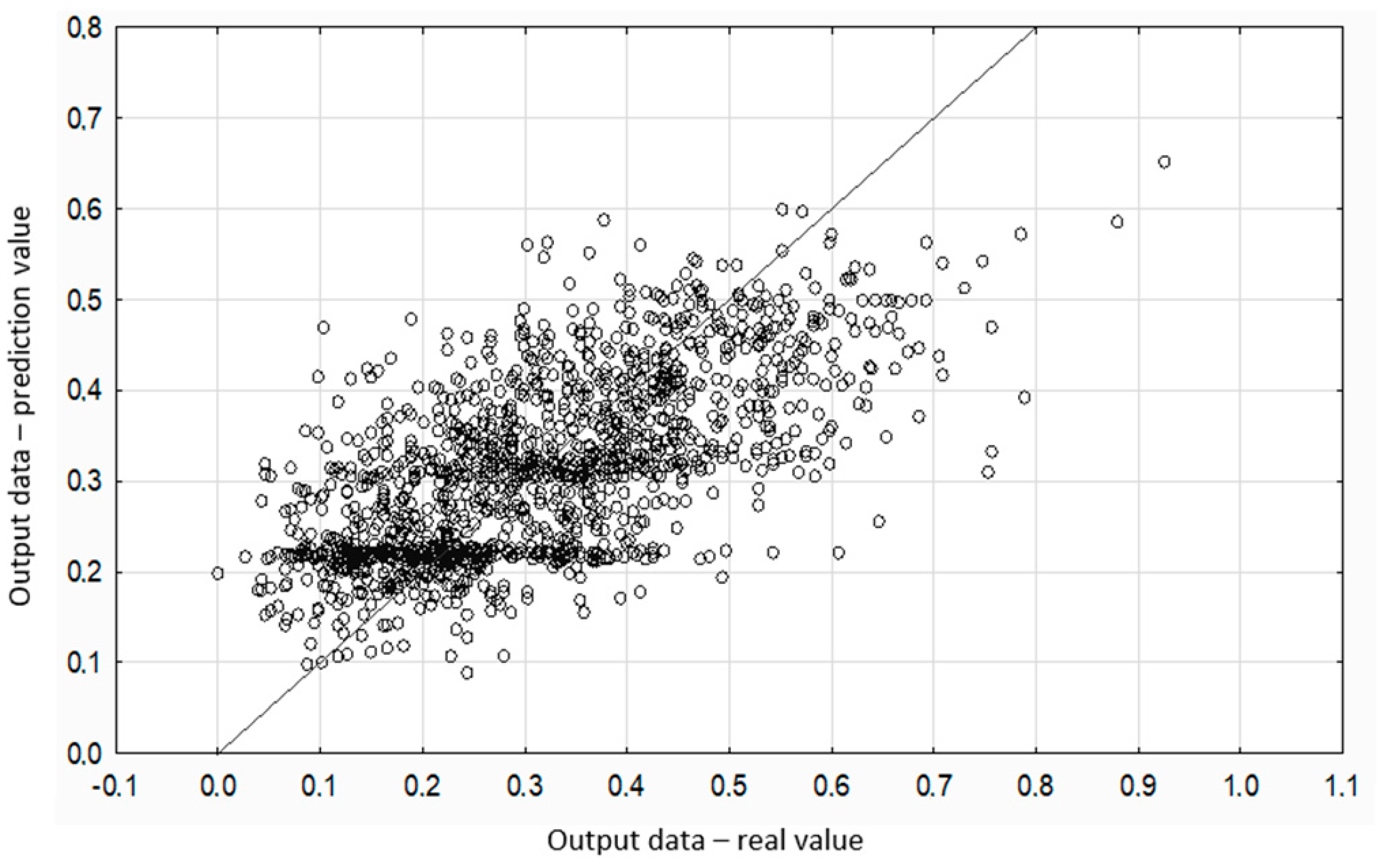
The #7 MLP 18-3-1 network was considered the best neural network and it was selected for further analysis (Table 1). The selected neural network consists of three layers: input (18 neurons), hidden (3 neurons) and output (1 neuron) layers. The accuracy of the network operation during the model validation stage was 93%, and the error value of the SOS was 0.007.
Figure 5 shows a diagram of the relationship between the actual and predicted values of the axle runout. The correlation model allows you to determine the expected values of one random variable on the basis of unit representations of another random variable with features of mutual correlation. The validation was performed using the set of input and output data, that were not used before. From the diagram, one can deduce the direction and strength of the correlation relationship. The points of the studied dependence are grouped along a hypothetical straight regression, indicating the strength of the correlation.
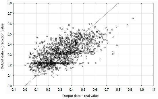
Figure 5.
Axle radial runout—prediction and real values comparison.
One of the most significant thing in the process of modeling the structure of an artificial neural network is assigning weights to interneural connections. The efficiency of the prediction of the output value is inextricably linked with the values of weights assigned to individual units of the network layer, where negative values weaken and positive values strengthen the transmitted signals. Table 2 shows the weight values generated for the analyzed MLP 18-3-1 network.
Table 2.
Set of interneural weights of network MLP 18-3-1.
On the basis of the generated values of the weights of interneural connections, the most important input parameters creating the structure of the neural network can be identified. Values greater than neutral zero indicate greater importance from the point of view of prediction of the output value. Analyzing the example of predicting the value of radial runout in the assembly operation of machine parts, the greatest significance of the parameters was observed: the dimension of the main reference diameter; the position of the hole for the axle that is being assembled, relative to the main reference diameter in the Y axis; the position of the hole for axle that is being assembled relative to the main reference diameter in the X axis; body bottom wall thickness on the left side of the symmetry axis; the dimension in five planes of the hole for the axle that is being assembled, along its entire depth (V plane). For the mentioned parameters, there was a particular strengthening or weakening of the value of the transmitted signal (weight value below −10 or above 10) to the next units of the neural network structure.
4. Conclusions
Artificial neural networks are an effective tool to support the control of the production process. The example of the prediction of the value of radial runout of machine parts presented in this paper confirms the above statement—the effectiveness of the network is greater than 90%. According to the authors, this effectiveness may be improved, for example, as a result of an increase in the amount of data that train NN and further analysis of the process.
The neural network can be successfully used in the industry on the basis of the implementation of the program code into a generally available application. By entering the input values (18 parameters) it is possible to obtain the predicted value of the radial runout. The use of the application in real production conditions will allow a reduction in the number of post-production tests but most of all an increase in their effectiveness, and thus will improve the quality of manufactured products and reduce production costs. In conclusion, one of the most important effects of the application of the developed method is obtaining the estimated value of the radial runout on the basis of specific production and assembly parameters.
To sum up, the model of a neural network presented in the work, selected during the research from 1000 analyzed models, is a very effective tool for improving the production process, the operation of which is presented on a real production example in one of the largest brass processing companies in Europe. Therefore, it is not purely theoretical scientific considerations, but is a kind of important case study of the application of science in industrial conditions on a large number of objects under study.
Author Contributions
Conceptualization, M.S.; methodology, M.S. and K.P.; software, K.P.; validation, M.S., K.P. and M.B.; formal analysis, F.K. and M.T.; investigation, M.S. and K.P.; resources, A.M.; data curation, K.P., M.S. and A.M.; writing—original draft preparation, M.S. and K.P; writing—review and editing, M.B.; visualization, A.M.; supervision, M.S.; project administration, M.S., K.P. and A.M.; funding acquisition, M.S. and K.P. All authors have read and agreed to the published version of the manuscript.
Funding
This work was supported by Ministry of Science and Higher Education of Poland (No. 614/SBAD/1565).
Institutional Review Board Statement
Not applicable.
Informed Consent Statement
Not applicable.
Conflicts of Interest
The authors declare no conflict of interest.
References
- Qi, X.; Chen, G.; Li, Y.; Cheng, X.; Li, C. Applying Neural-Network-Based Machine Learning to Additive Manufacturing: Current Applications, Challenges, and Future Perspectives. Engineering 2019, 5, 721–729. [Google Scholar] [CrossRef]
- Scime, L.; Beuth, J. A multi-scale convolutional neural network for autonomous anomaly detection and classification in a laser powder bed fusion additive manufacturing process. Addit. Manuf. 2018, 24, 273–286. [Google Scholar] [CrossRef]
- Mundada, V.; Narala, S.K.R. Optimization of Milling Operations Using Artificial Neural Networks (ANN) and Simulated Annealing Algorithm (SAA). Mater. Today Proc. 2018, 5, 4971–4985. [Google Scholar] [CrossRef]
- Pfrommer, J.; Zimmerling, C.; Liu, J.; Kärger, L.; Henning, F.; Beyerer, J. Optimisation of manufacturing process parameters using deep neural networks as surrogate models. Procedia CIRP 2018, 72, 426–431. [Google Scholar] [CrossRef]
- Wojciechowski, J.; Suszyński, M.; Żurek, J.; Vjesnik, T. No Clamp Robotic Assembly with Use of Point Cloud Data from Low-Cost Triangulation Scanner. Teh. Vjesn. 2018, 25, 904–909. [Google Scholar]
- Iwańkowicz, R. Optimization of assembly plan for large offshore structures. Adv. Sci. Technol. Res. J. 2012, 6, 31–36. [Google Scholar] [CrossRef]
- Ciszak, O.; Suszyński, M. Selection of Assembly Sequence for Manual Assembly Based on DFA Rating Factors. In Advances in Manufacturing II. Volume 2-Production Engineering and Management; Springer: Midtown Manhattan, NY, USA, 2019. [Google Scholar]
- Chen, S.-F.; Liu, Y.-J. An adaptive genetic assembly-sequence planner. Int. J. Comput. Integr. Manuf. 2001, 14, 489–500. [Google Scholar] [CrossRef]
- Wang, D.; Shao, X.; Liu, S. Assembly sequence planning for reflector panels based on genetic algorithm and ant colony optimization. Int. J. Adv. Manuf. Technol. 2017, 91, 987–997. [Google Scholar] [CrossRef]
- Xin, L.; Jianzhong, S.; Yujun, C. An efficient method of automatic assembly sequence planning for aerospace industry based on genetic algorithm. Int. J. Adv. Manuf. Technol. 2017, 90, 1307–1315. [Google Scholar] [CrossRef]
- Sinanoglu, C.; Börklü, H.R. An assembly sequence-planning system for mechanical parts using neural network. Assem. Autom. 2005, 25, 38–52. [Google Scholar] [CrossRef]
- Suszyński, M.; Peta, K. Assembly Sequence Planning Using Artificial Neural Networks for Mechanical Parts Based on Selected Criteria. Appl. Sci. 2021, 11, 10414. [Google Scholar] [CrossRef]
- Suszyński, M.; Peta, K.; Černohlávek, V.; Svoboda, M. Mechanical Assembly Sequence Determination Using Artificial Neural Networks Based on Selected DFA Rating Factors. Symmetry 2022, 14, 1013. [Google Scholar] [CrossRef]
- Chen, W.-C.; Tai, P.-H.; Deng, W.-J.; Hsieha, L.-F. A three-stage integrated approach for assembly sequence planning using neural networks. Expert Syst. Appl. 2008, 34, 1777–1786. [Google Scholar] [CrossRef]
- Kucukoglu, I.; Atici-Ulusua, H.; Gunduz, T.; Tokcalar, O. Application of the artificial neural network method to detect defective assembling processes by using a wearable technology. J. Manuf. Syst. 2018, 49, 163–171. [Google Scholar] [CrossRef]
- Židek, K.; Hosovsky, A.; Piteľ, J.; Bednár, S. Recognition of Assembly Parts by Convolutional Neural Networks. In Advances in Manufacturing Engineering and Materials; Springer: Cham, Switzerland, 2018; pp. 281–289. [Google Scholar]
- Patel, A.; Andrews, P.; Summers, J.D.; Harrison, E.; Schulte, J.; Mears, M.L. Evaluating the Use of Artificial Neural Networks and Graph Complexity to Predict Automotive Assembly Quality Defects. J. Comput. Inf. Sci. Eng. 2017. [Google Scholar] [CrossRef]
- Tadeusiewicz, R.; Chaki, R.; Chaki, N. Exploring Neural Networks with C#; CRC Press: Boca Raton, FL, USA, 2015. [Google Scholar]
- Lu, Z.; Jiang, J.; Cao, P.; Yang, Y. Assembly Quality Detection Based on Class-Imbalanced Semi-Supervised Learning. Appl. Sci. 2021, 11, 10373. [Google Scholar] [CrossRef]
- Jiang, J.; Cao, P.; Lu, Z.; Lou, W.; Yang, Y. Surface Defect Detection for Mobile Phone Back Glass Based on Symmetric Convolutional Neural Network Deep Learning. Appl. Sci. 2020, 10, 3621. [Google Scholar] [CrossRef]
- Zhan, G.; Wang, W.; Sun, H.; Hou, Y.; Feng, L. Auto-CSC: A Transfer Learning Based Automatic Cell Segmentation and Count Framework. Cyborg Bionic Syst. 2022, 2022, 9842349. [Google Scholar] [CrossRef] [PubMed]
- Bai, D.; Liu, T.; Han, X.; Yi, H. Application Research on Optimization Algorithm of sEMG Gesture Recognition Based on Light CNN + LSTM Model. Cyborg Bionic Syst. 2021, 2021, 9794610. [Google Scholar] [CrossRef] [PubMed]
- Iwańkowicz, R.; Taraska, M. Self-classification of assembly database using evolutionary method. Assem. Autom. 2018, 38, 268–281. [Google Scholar] [CrossRef]
- Broomhead, D.S.; Lowe, D. Radial Basis Functions, Multi-Variable Functional Interpolation and Adaptive Networks; Report, Royal Signals and Radar Establishment: Malvern, PA, USA, 1988. [Google Scholar]

Publisher’s Note: MDPI stays neutral with regard to jurisdictional claims in published maps and institutional affiliations. |
© 2022 by the authors. Licensee MDPI, Basel, Switzerland. This article is an open access article distributed under the terms and conditions of the Creative Commons Attribution (CC BY) license (https://creativecommons.org/licenses/by/4.0/).