Research on Generalized Hybrid Probability Convolutional Neural Network

Abstract

This paper first studies the generalization ability of the convolutional layer as a feature mapper (CFM) for extracting image features and the classification ability of the multilayer perception (MLP) in a CNN. Then, a novel generalized hybrid probability convolutional neural network (GHP-CNN) is proposed to solve abstract feature classification with an unknown distribution form. To measure the generalization ability of the CFM, a new index is defined and the positive correlation between it and the CFM is researched. Generally, a fully trained CFM can extract features that are beneficial to classification, regardless of whether the data participate in training the CFM. In the CNN, the fully connected layer in the MLP is not always optimal, and the extracted abstract feature has an unknown distribution. Thus, an improved classifier called the structure-optimized probabilistic neural network (SOPNN) is used for abstract feature classification in the GHP-CNN. In the SOPNN, the separability information is not lost in the normalization process, and the final classification surface is close to the optimal classification surface under the Bayesian criterion. The proposed GHP-CNN utilizes the generalization ability of the CFM and the classification ability of the SOPNN. Experiments show that the proposed network has better classification ability than the existing hybrid neural networks.

1. Introduction

The effect of pattern classification is mainly determined by classification features and classifiers. For an image classification task, the classification model needs to extract image features that are easy to distinguish, and then design a suitable classifier that matches the features. Traditional artificial feature extraction methods have achieved good results, such as the local binary pattern (LBP) [1,2], the speeded-up robust features (SURF) [3,4] and the scale-invariant features (SIFT) [5,6]. However, these features are single features without any hierarchical structure, sometimes lacking good generalization abilities. In recent years, the convolutional neural network (CNN) has attracted the extensive attention of scholars in many fields [7,8,9,10], because CNNs can extract various shallow features and deep features of images.

Based on the MLP training algorithm, LeCun et al. [11] designed a convolutional neural network called LeNet-5, which was an early classic convolutional neural network model. It was mainly used for handwritten digit recognition on checks. With a gradual increase in the number of convolutional layers, the CNN’s feature extraction classification abilities are becoming stronger and stronger. Similarly, graph convolution networks (Graph CNNs) have good feature extraction ability [12,13,14], because a Graph CNN is also very effective for non-Euclidean data, and is relatively more complex. In this paper, we only discuss CNNs. Krizhevsky [15] proposed the extended deep convolutional neural network AlexNet, which used the ReLU function instead of the saturated nonlinear function tanh. It also used the dropout technique to avoid overfitting in the training process. In 2014, Google proposed a convolutional neural network with more than 20 layers, GoogLeNet [16], to resolve the gradient disappearance and two loss functions were designed at different depths of the network. The VGG [17] network model proposed by Oxford University adopted a layer-by-layer training method. The trained VGG network showed a good ability to extract image features. The residual network ResNet proposed in [18] allowed the original input information to be passed directly to the subsequent network layer by adding connected channels directly. ResNet could train hundreds or even thousands of layers while achieving a good classification accuracy. In general, the above various types of convolutional neural networks have achieved good results in different scenarios, mainly because the convolutional layer of a CNN can extract abstract features with good separability. However, because the distribution of these abstract features is unpredictable, designing a suitable classifier for these features is a problem worthy of further study.

The above CNNs can extract all kinds of image features that are good for image classification, but the MLP classifiers in CNNs sometimes fall into local optimal [19,20,21,22,23,24,25,26,27]. To solve this problem, Niu et al. [19] proposed using a pretrained CNN as the feature extractor to extract the hierarchical features of an image, and then using an SVM as the classifier. The beginning of the method mainly focused on the binary classification problem. When applied to multiclass classification problems, it mainly adopted multiple two-classifier voting methods. In a multiple-two-classification problem, if a sample has the highest number of votes in two different categories, the SVM divides the sample into either category, which may lead to classification errors. Duan et al. [20] proposed using the pretrained CNN as a feature extractor to extract facial features, and then using an extreme learning machine (ELM) as a classifier. However, it was generally necessary to reset the number of hidden nodes when using ELM classifiers on different dataset. Tien et al. [26] used depth features and artificial features to merge into new hybrid features, and then used an SVM as a classifier. The new hybrid features combined the characteristics of deep features and artificial features and had a high separability. Guo et al. [27] proposed a multinetwork feature fusion structure that used merged features to classify features. Merged features have more information than a single feature, which is beneficial in classification tasks. Although studies have shown that convolutional neural networks have a good ability to extract image features and have good classification capabilities, training a deep convolutional neural network takes a long time and requires a large quantity of data. When a new dataset needs to be classified, the network needs to be retrained.

The above literature review shows that the convolutional layer as a CFM, which is fully trained by a multicategory source dataset, can extract image features that are beneficial to the classification, but there are no studies on the relationship between the generalization ability of the CFM-extracted features, the number of source dataset and target dataset categories. In this paper, the trained CNN on the multiclass source dataset does not need retraining. It directly extracts image features from new target tasks and then cascades the appropriate classifier. This can not only use the ability of the CNN convolutional layer to extract image features, but also makes use of the advantages of different classifiers.

The main contributions of this paper include the following three points. First, the general rule between the generalization ability of the CNN’s convolutional layer as a CFM, and the number of categories of the source dataset and target dataset are summarized. Then, the interpretability of the generalization ability of the CFM is given. Second, a new GHP-CNN is proposed to solve the problem of a target image classification. The GHP-CNN mainly includes a CFM that extracts the features of the target set and a classifier called the structure-optimized probability neural network (SOPNN). The SOPNN classifier is not restricted by the distribution form of the target feature. The GHP-CNN avoids the problem of MLP classifiers in CNN networks easily falling into local optima and improves the classification ability.

The organizational structure of the rest of this paper is as follows. In Section 2, the generalization ability of the CFM to extract target image features is studied. In Section 3, a structure-optimized probabilistic neural network classifier is designed. In Section 4, the GHP-CNN is proposed, and its principle and characteristics are analyzed. Section 6 presents the analytical and experimental results. The last section summarizes the conclusions of the study. Some important symbols used in this article are shown in Table 1.

Table 1. Important notations and variables used in this paper.

${\mathit{S}}^{*}$	The source dataset for training the CNN
s	The number of classes in the source dataset $S^{*}$
$T^{*}$	The target dataset for classification
t	The number of classes in the target dataset $T^{*}$
$P_s$	The original training accuracy of VGG-16 in the source dataset with s class samples
$P_t^s$	The test accuracy of target sets with t class samples
${\tilde{P}}_t^s$	The average accuracy of multiple $P_t^s$
$\mathbf{CFM}$	Convolutional feature mapper
${\mathbf{CFM}}_s$	Convolutional feature mapper trained by the source dataset with s class samples
$T^{*}\subset S^{*}$	The samples in $T^{*}$ are selected from $S^{*}$
$S^{*}\bigcap T^{*}=\varnothing$	The number of common samples between $T^{*}$ and $S^{*}$ is zero
$r_t^s$	The increased amplitude of the t class target dataset compared with the s class source dataset
$tr\left(\mathbf{A}\right)$	The trace of matrix $\mathbf{A}$
$det\left(\mathbf{A}\right)$	The determinant of matrix $\mathbf{A}$

2. Research on the Generalization Ability of the CNN Feature Mapper (CFM) to Extract Image Features

In this paper, the dataset $S^{*}$ for training the CNN is called the source dataset, and the dataset $T^{*}$ for testing the CFM generalization ability is called the target dataset. The number of sample categories in $S^{*}$ is $s(s=s1,\cdots ,sm)$ and the number of sample categories in $T^{*}$ is $t(t=t1,\cdots ,tm)$. In general, the sample categories in the source dataset $S^{*}$ and the target dataset $T^{*}$ are not the same. This paper comprehensively studies the relationship between category reduction, unknown category expansion and the generalization ability of CNNs to extract target image features. In this paper, the category reduction refers to the source dataset $S^{*}$ containing the target dataset $T^{*}$($T^{*}\subset S^{*}$). An unknown category extension means that there is no sample that is common to both the source dataset and the target dataset ($S^{*}\bigcap T^{*}=\varnothing$). The network used in this section was VGG-16 [17] (stride =1, padding = 1, MaxPooling), and the dataset used was CIFAR-100 [28].

The convolution neural network trained on the source dataset $S^{*}$ can be simply divided into two parts: the convolutional layer used to extract the feature and the MLP layer as the classifier. The convolutional network is fully trained on the source dataset until it converged, and the convolutional layer migrates as the CFM of the target set. As shown in Figure 1, after the source dataset $S^{*}$ is trained by the convolutional network and the MLP layer, the corresponding classification accuracy $P_s$ is obtained, the feature mapper corresponding to the source dataset $S^{*}$ of the s class is ${\mathbf{CFM}}_{\mathbf{s}}$, and the target dataset $T^{*}$ of the t class is passed through the ${\mathbf{CFM}}_{\mathbf{s}}$. The features are extracted, and then classification training is performed with the MLP classifier, and the corresponding accuracy $P_s^t$ is obtained

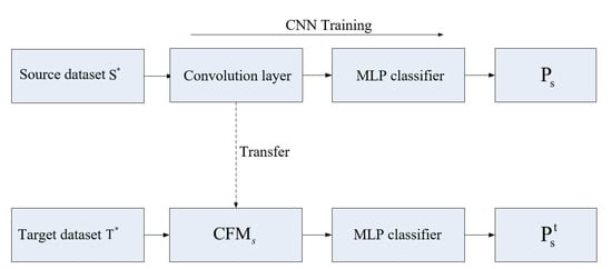
Figure 1. The experimental structure diagram of generalization ability of feature mapper.

For the different affiliations between the source dataset $S^{*}$ and the target dataset $T^{*}$, and to make the experiment statistically valid, when training multiple ${\mathbf{CFM}}_{\mathbf{s}}$, s different categories of the source dataset and t categories of the target dataset were selected, where each s and t category samples satisfied the uniform distribution in the CIFAR-100 dataset. Multiple source datasets $S_{s1}^{*},S_{s2}^{*},\cdots ,S_{sm}^{*}$ were selected, where $S_{s1}^{*}\subset S_{s2}^{*}\subset ,\cdots ,\subset S_{sm}^{*}$. When $T^{*}\subset S^{*}$, multiple target datasets $T_{t1}^{*},T_{t2}^{*},\cdots ,T_{tm}^{*}$ were selected, where $T_{t1}^{*}\subset T_{t2}^{*}\subset ,\cdots ,\subset T_{tm}^{*}$.

For each t-class target dataset, there are an average classification accuracy ${\tilde{P}}_s^t$ and a classification accuracy $P_s$ of the s-class source dataset corresponding to the ${\mathbf{CFM}}_{\mathbf{s}}$. Comparisons between the magnitudes of ${\tilde{P}}_s^t$ and $P_s$ show the generalization ability of the ${\mathbf{CFM}}_{\mathbf{s}}$ in the t-class target dataset.

$$r_s^t=\frac{{\tilde{P}}_s^t-P_s}{P_s}$$

(1)

The size of $r_s^t$ can measure the strength of the ${\mathbf{CFM}}_{\mathbf{s}}$’s generalization ability. That is, the greater the value of $r_s^t$ is, the stronger the generalization ability of the ${\mathbf{CFM}}_{\mathbf{s}}$. When $r_s^t>0$, the ${\mathbf{CFM}}_{\mathbf{s}}$ can extract features with better separability for the t-class targets and can obtain a higher accuracy than $P_s$ under subsequent classifiers. That is, a $\mathbf{CFM}$ trained by the s-class source dataset $S^{*}$ has a better generalization ability for a t-class target dataset $T^{*}$. When $r_s^t<0$, the ${\mathbf{CFM}}_{\mathbf{s}}$ fails to extract features with better separability in the t-class target dataset, which results in a lower accuracy than the original $P_s$ under subsequent classifiers. The corresponding classification accuracy can be obtained by changing the membership relationship between $S^{*}$ and $T^{*}$, and the generalization ability of the ${\mathbf{CFM}}_{\mathbf{s}}$ under different conditions can be further reflected by increasing or decreasing the magnitude of the classification accuracy compared with the original accuracy.

2.1. Analysis of the Generalization Ability of the Feature Mapper to the Target Set after Category Reduction ($T^{*}\subset S^{*}$)

When $T^{*}\subset S^{*}$, the trained ${\mathbf{CFM}}_{\mathbf{s}}$ on multiclass source dataset $S^{*}$ extracts the features of target dataset $T^{*}$ and trains the classification by the MLP classifier. In the CIFAR-100 dataset, we selected the source dataset with the number of categories for s ($s=15,20,25,\cdots ,100$) to be fully trained with the VGG-16 algorithm, we obtained different original precisions $P_s$ and the corresponding 15 ${\mathbf{CFM}}_{\mathbf{s}}$s, and then randomly extracted the target dataset $T^{*}$ with the number of categories t ($t=5,10,\cdots ,30$) from the source dataset $S^{*}$. The features of these target dataset $T^{*}$ were extracted by the ${\mathbf{CFM}}_{\mathbf{s}}$, and then the training classification was performed by the MLP classifier. To make the results more universal, the target dataset of each category are randomly extracted eight times. The classification accuracy $P_s^t$ was counted each time, and the final result was the average value of the multiple classification results, where t represented the number of categories in the target dataset $T^{*}$, and s represented the number of categories in the source dataset $S^{*}$.

As shown in Figure 2, it can be seen that for the determined t categories from target dataset $T^{*}$, the value of $r_s^t$ was positively correlated with s: as the corresponding s of the ${\mathbf{CFM}}_{\mathbf{s}}$ increased, $r_s^t$ increased monotonously. That is, for a certain target dataset with t categories, the larger the value of s was, the better the generalization ability of the ${\mathbf{CFM}}_{\mathbf{s}}$ trained by the source dataset $S^{*}$. For a $\mathbf{CFM}$ trained on the determined s source dataset $S^{*}$, the value of $r_s^t$ was negatively correlated with $T^{*}$ and with the number of t categories in the target dataset; $r_s^t$ decreased monotonously as t increased. That is, for a ${\mathbf{CFM}}_{\mathbf{s}}$ that determined the number of categories, a target dataset $T^{*}$ with a smaller number of t had a better the generalization ability than a target dataset with larger values of t. When $r_s^t$ was a certain value, that is, after the feature was extracted under the ${\mathbf{CFM}}_{\mathbf{s}}$ for t different categories, and the magnitude of the classification promotion was the same, the number of ${\mathbf{CFM}}_{\mathbf{s}}$ for different values of t corresponding to s was different.

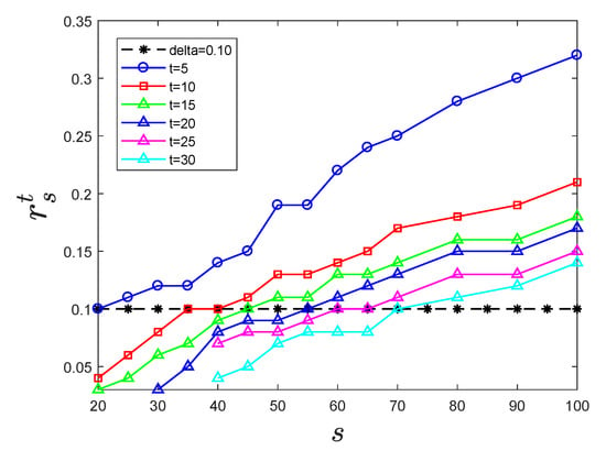
Figure 2. The accuracy increase of different t unknown subclasses compared with the original accuracy.

2.2. Analysis of the Generalization Ability of the Feature Mapper to Unknown Target Categories ($S^{*}\bigcap T^{*}=\varnothing$)

When $S^{*}\bigcap T^{*}=\varnothing$, the trained ${\mathbf{CFM}}_{\mathbf{s}}$ on a multiclass source dataset $S^{*}$ extracts the features of target dataset $T^{*}$ and the features are used for training the MLP classifier. In the CIFAR-100 dataset, 90 categories were randomly selected as a candidate source dataset, and the remaining 10 categories were used as a candidate target dataset. The sample sets with number of categories s ($s=15,20,25,\cdots ,90$) were selected from the 90 candidate source dataset to be fully trained by VGG-16, and the relatively best classification results and corresponding 14 ${\mathbf{CFM}}_{\mathbf{s}}$ were obtained and randomly selected from the 10 candidate dataset. The unknown target dataset with a number of categories t ($t=2,3,\cdots ,8$) was selected, and the features of the randomly selected unknown target dataset were extracted by the CFM and then trained by the MLP classifier. To make the results more universal, each number of unknown sample subsets was extracted three times, the classification results were counted each time, and the final result was the average of three results.

As shown in Figure 3, for the determined t category target dataset $T^{*}$, the value of $r_s^t$ was positively correlated with s; as the corresponding s of the ${\mathbf{CFM}}_{\mathbf{s}}$ increased, $r_s^t$ increased monotonously. That is, for a certain t category target dataset, the larger s was, the better the generalization ability of the ${\mathbf{CFM}}_{\mathbf{s}}$ trained by the source dataset $S^{*}$. For the ${\mathbf{CFM}}_{\mathbf{s}}$ trained from the determined s category source dataset $S^{*}$, the value of $r_s^t$ was negatively correlated with the number of t categories in the target dataset $T^{*}$; as t increased, $r_s^t$ decreased monotonously. That is, for a ${\mathbf{CFM}}_{\mathbf{s}}$ that determined the number of categories, the generalization ability of the target dataset $T^{*}$ with a smaller t was better. When $r_s^t$ was a certain value, that is, after the feature was extracted under the ${\mathbf{CFM}}_{\mathbf{s}}$ for different t categories from the target dataset, and the magnitude of the classification promotion was the same, then the number of ${\mathbf{CFM}}_{\mathbf{s}}$ for t categories corresponding to s categories was different.

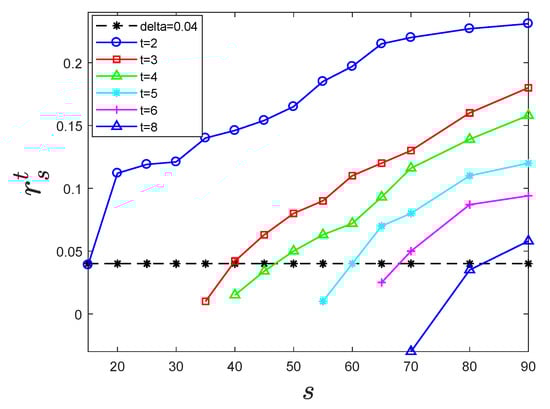
Figure 3. The accuracy increase of different t unknown subclasses compared with the original accuracy.

2.3. Analysis of the CFM Generalization Ability

Through the above experiments, which were from different angles, the generalization ability of CFM was analyzed in a large number of ways. From the analysis, the generalization ability of a trained CNN as a CFM was related to the number of categories in the source dataset(t). The more categories in the source dataset were trained by the CFM, the better the generalization ability of the CFM, and the closer it was to global optimum characteristics.

In the above experiments, the features extracted by the CFM were input to the MLP for intensive training, which could be regarded as a fine-tuning of the MLP classifier after parameter migration. Although the network after fine-tuning the MLP classifier also had a better classification accuracy, it might also fall into a local optimum, and the internal function mapping relationship would be difficult to explain. Since the image features extracted by ${\mathbf{CFM}}_{\mathbf{s}}$ are generally abstract, the feature distribution is unknown. The classifier based on the Bayesian probability density is not restricted by the distribution of target features, and the final classification surface is close to the optimal classification surface under the Bayesian criterion. We design an optimized Bayesian classifier in the next section.

3. SOPNN Classifier in the GHP-CNN

3.1. The Overall Structure of the SOPNN Classifier

As shown in Figure 4, the SOPNN classifier consists of four layers. The first layer is the input layer for receiving the input feature vectors. A traditional PNN adopts a unit hypersphere normalization for the pattern vectors and input samples, which ensures that the distance between different vectors in a network can be expressed in a simple inner product form. That is, the squared distance between $\mathbf{x}$ and $\mathbf{y}$ can be expressed as $\Vert \mathbf{x}-\mathbf{y}\Vert =2-2{\mathbf{x}}^T\mathbf{y}$ if $\mathbf{x}$ and $\mathbf{y}$ are normalized. Note that such a simple inner form can be easily realized with a neuron structure. However, with a hypersphere normalization, all sample points that are collinear with the sphere center overlap. To avoid the separability problem in the hypersphere normalization process, the SOPNN used the unit hyperspherical crown normalization $\widehat{\mathbf{x}}=\overline{\mathbf{x}}/\parallel \overline{\mathbf{x}}\parallel$ from reference [29], where $\overline{\mathbf{x}}=[\mathbf{x},h]\in {\mathbf{R}}^{n+1}$ and $\mathbf{x}$ are n-dimensional features of the target image extracted by the CFM. h is the additional dimension.

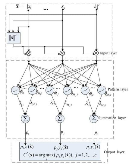
Figure 4. The overall structure of the SOPNN classifier.

The second layer is the pattern layer, and the pattern nodes in this layer receives the vector $\widehat{\mathbf{x}}$ from the input layer. Let a pattern node ${\widehat{\mathbf{u}}}^{mj}$ be the mth center in the jth class ($1\le j\le c,1\le m\le M_j$). Its output can be given by

$${\varphi }_{mj}\left(\widehat{\mathbf{x}}\right)=\frac{exp\left[-\frac{{\left(\widehat{\mathbf{x}}-{\widehat{\mathbf{u}}}^{mj}\right)}^T\left(\widehat{\mathbf{x}}-{\widehat{\mathbf{u}}}^{mj}\right)}{2{\left({\sigma }_{mj}\right)}^2}\right]}{{\left(2\pi \right)}^{(\mathrm{n}+1)/2}{\left({\sigma }_{mj}\right)}^{(n+1)}}$$

(2)

where ${\sigma }_{mj}$ denotes the kernel width, $M_j$ denotes the number of pattern nodes in the jth class and the total number of pattern nodes is M. That is, $M={\sum }_{j=1}^c{M}_j$.

The third layer is the summation layer, which includes c neurons and one neuron per class. Each neuron calculates a conditional probability density function $y_j\left(\widehat{\mathbf{x}}\right)$ for each class using the following weighted summation form.

$$y_j\left(\widehat{\mathbf{x}}\right)=\sum _{m=1}^{M_j}{\lambda }_{mj}{\varphi }_{mj}\left(\widehat{\mathbf{x}}\right),1\le j\le c$$

(3)

where ${\lambda }_{mj}$ denotes the prior distribution information of the training samples of the mth center in the jth class and satisfies ${\sum }_{m=1}^{M_j}{\lambda }_{mj}=1(1\le j\le c)$.

The fourth layer is the output layer, which makes decisions according to the following equation.

$$C^{*}\left(\mathbf{x}\right)=argmax\left\{p_j{y}_j\left(\widehat{\mathbf{x}}\right)\right\},j=1,2,\cdots ,c$$

(4)

where c is the class number and $C^{*}\left(\mathbf{x}\right)$ is the predicted class of $\mathbf{x}$. $p_j$ denotes the prior probability of the jth class. Obviously, all the parameters have an interpretable physical meaning in our classifier.

3.2. The Hidden Parameter Optimization in the SOPNN Using the EM Algorithm

The EM algorithm solves the parameter estimation problem using iterative methods in various probability models. Each iteration consists of two steps, called the $\mathbf{E}$ step and the $\mathbf{M}$ step. The $\mathbf{E}$ step uses the existing estimated parameters and the observed data to calculate the expectation of the hidden parameters. The $\mathbf{M}$ step uses the expectation obtained in the $\mathbf{E}$ step and maximum likelihood estimation to estimate the hidden parameter.

Let a set X that is used for training the SOPNN contain L samples from c classes, and let the jth class contain $L_j$ training samples. That is, $X={\left\{{\mathbf{x}}^l\right\}}_{l=1}^L={\left\{{\left\{{\mathbf{x}}^{lj}\right\}}_{l=1}^{L_j}\right\}}_{j=1}^c$. With a hyperspherical crown mapping, X can be projected as $\widehat{X}={\left\{{\widehat{\mathbf{x}}}^l\right\}}_{l=1}^L={\left\{{\left\{{\widehat{\mathbf{x}}}^{lj}\right\}}_{l=1}^{L_j}\right\}}_{j=1}^c$. According to the independence of the sample, the corresponding log-likelihood function can be obtained:

$$Log=\sum _{j=1}^c\sum _{l=1}^{L_j}log{y}_j\left({\widehat{\mathbf{x}}}^{lj}\right)=\sum _{j=1}^c\sum _{l=1}^{L_j}log\sum _{m=1}^{M_j}{\lambda }_{mj}{\varphi }_{mj}\left({\widehat{\mathbf{x}}}^{lj}\right)$$

(5)

Using the EM algorithm to solve for the maximum value of the likelihood function, the following iterative formulas can be obtained:

$${\widehat{\mathbf{u}}}^{mj}=\frac{{\sum }_{l=1}^{L_j}{w}_{mj}\left({\widehat{\mathbf{x}}}^{lj}\right){\widehat{\mathbf{x}}}^{lj}}{{\sum }_{l=1}^{L_j}{w}_{mj}\left({\widehat{\mathbf{x}}}^{lj}\right)}$$

(6)

$${\sigma }_{mj}^2=\frac{{\sum }_{l=1}^{L_j}{w}_{mj}\left({\widehat{\mathbf{x}}}^{lj}\right){\left({\widehat{\mathbf{x}}}^{lj}-{\widehat{\mathbf{u}}}^{mj}\right)}^T\left({\widehat{\mathbf{x}}}^{lj}-{\widehat{\mathbf{u}}}^{mj}\right)}{(n+1){\sum }_{l=1}^{L_j}{w}_{mj}\left({\widehat{\mathbf{x}}}^{lj}\right)}$$

(7)

$${\lambda }_{mj}=\frac{{\sum }_{l=1}^{L_j}{w}_{mj}\left({\widehat{\mathbf{x}}}^{lj}\right)}{L_j}$$

(8)

$$w_{mj}\left({\widehat{\mathbf{x}}}^{lj}\right)=\frac{{\lambda }_{mj}{\varphi }_{mj}\left({\widehat{\mathbf{x}}}^{lj}\right)}{{\sum }_{m=1}^{M_j}{\lambda }_{mj}{\varphi }_{mj}\left({\widehat{\mathbf{x}}}^{lj}\right)}$$

(9)

If the initial pattern node and kernel width are known, we can obtain the corresponding parameter value ${\lambda }_{mj}$ in Equation (4) by using the above iterative formulas. The termination criterion of the EM algorithm is that the absolute value of the difference between the hidden parameter ${\theta }^{(i+1)}$ of the $(i+1)$th order and the hidden parameter ${\theta }^{\left(i\right)}$ of the $\left(i\right)$th order is less than a given positive $ϵ$, where $ϵ=0.01$.

There are three differences between the used SOPNN classifier in this paper and the traditional probability neural network (PNN) classifier. First, the hyperspherical crown normalization method in the SOPNN is a map without separable information loss, and the hypersphere normalization in a traditional PNN is a map with separable information loss. The conclusion that the hyperspherical crown normalization is superior to the traditional hypersphere normalization in terms of separability was proven in [29]. Second, when the training set is large, the number of pattern nodes in the traditional PNN is equal to the number of training samples, which leads to a complex network structure. In this paper, the kernel coverage method based on the potential function in [30] is used to adaptively generate pattern nodes, which makes the number of pattern nodes far fewer than the number of training samples. This ensures that the network structure of the SOPNN is simpler than that of the traditional PNN. Third, the SOPNN assigns a local intraclass weight coefficient to each pattern node, which reflects the prior distribution information of the local region of the pattern node. Therefore, the probability density estimation in the SOPNN is more accurate than in the traditional PNN, and its classification surface can better approximate the optimal classification surface under the Bayesian criterion. The hidden parameters ${\lambda }_{mj}$ and ${\sigma }_{mj}$ in the SOPNN can be optimized by using the expectation maximization algorithm.

4. GHP-CNN Neural Network

Structure and Characteristics of the GHP-CNN

The network structure of the GHP-CNN in this paper is shown in Figure 5. The GHP-CNN mainly consists of three steps in the training process. First, the CNN is adequately trained with the source data. The source data information is propagated forward and backward until the CNN converges. Second, the parameters of the convolutional layer can be obtained in the first step of training, and the convolutional layer with fixed parameters is transferred as a separate $\mathbf{CFM}$ to extract the image features of the training samples in the target set. Third, the SOPNN is trained on the target dataset. The image features of the target training set are input into the SOPNN for training, and a well-trained SOPNN classifier can be obtained. SOPNN training only requires forward propagation once and does not require backpropagation. After completing the above three steps, we obtain the trained GHP-CNN network. If the test image in the target dataset is input directly into the CFM, then the SOPNN classifier in the GHP-CNN can be used for target classification. The proposed GHP-CNN has the following three characteristics.

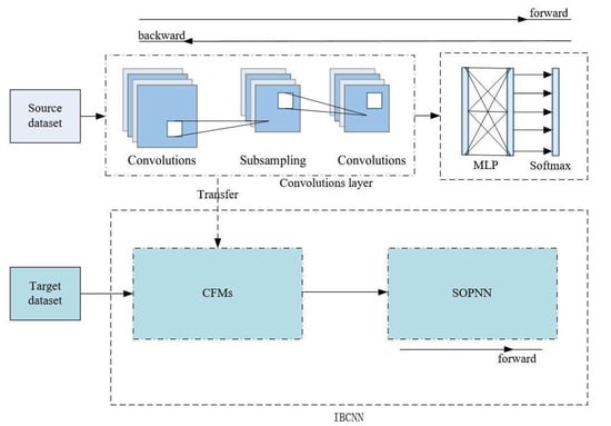
Figure 5. The network structure of GHP-CNN.

First, the GHP-CNN makes full use of the generalization ability and the parameter transferability of the CFM to extract image features. It only needs to transfer the convolutional layer as a CFM, and we do not need to transfer the entire CNN network.

Second, there is no need to retrain the CNN on the target set, only the SOPNN needs to be trained. The GHP-CNN can still be trained and work well even if the target dataset is small. Since training the SOPNN does not require backpropagation, the efficiency of training the SOPNN on the target set is significantly better than that of retraining the CNN.

Third, the distribution of the features extracted by the CFM is unknown. The SOPNN classifier in the GHP-CNN is based on probability density estimation and it is not limited by the distribution of the extracted features. Moreover, the interface of the SOPNN is close to the optimal classification surface under the Bayesian criterion, and there is no local optimal problem with the MLP classifier in the CNN.

Given the target set and initial network. The main steps of the GHP-CNN learning algorithm can be summarized as follows:

Step 1. According to the relationship between $delta$, s and t (as shown in Figure 2 and Figure 3), we can determine the number of categories in the source dataset and train various CFMs with different generality abilities.

Step 2. The CFM trained in the source dataset are transferred to extract the features of the target training set with the determined category number.

Step 3. The extracted features in step 2 are input into the SOPNN and are normalized by a hyperspherical crown normalization mapping. The appropriate parameter h should guarantee that the normalized data have the optimal separability under the Fisher criterion.

Step 4. The initial pattern node set of the SOPNN is generated by the adaptive kernel coverage method [30]. Because the number of generated pattern nodes is far less than the number of training samples, the SOPNN classifier with the optimized structure is obtained. A potential value is used to measure the distribution density of samples in the sample space, and the sample with the highest potential value is selected as the pattern node each time. Then, the potential value of the selected pattern region is iteratively eliminated, and the remaining samples are reordered according to the potential value.

Step 5. The parameters of the SOPNN are optimized by the expectation maximization method (Equations (7)–(10)), and then the well-trained GHP-CNN is obtained.

Step 6. The extracted features of the target test set are input into the SOPNN classifier in the GHP-CNN for classification.

5. Experiment and Results

5.1. Research on the GHP-CNN’s Classification Capabilities after Category Reduction

Through the analysis of the CFM’s generalization ability in the second part, the more source dataset categories used for training the CFM, the better the generalization ability. In the experiment, we used the CIFAR-100 and Caltech-256 datasets and the VGG and ResNet networks. After fully training VGG-16 with the CIFAR-100 dataset, the average accuracy of the 100-class test was 69.58%, and the fully trained convolutional layer was used as the CFM. Four, six, eight, twelve and sixteen subcategories were randomly selected from the CIFAR-100 data, and the corresponding classification accuracy of the subclasses was obtained after training with VGG-16. The features of these subclasses were extracted by the CFM and trained and tested with hybrid networks such as VGG-16-E, CNN-PNN, CNN-SVM, CNN-ELM and GHP-CNN. VGG-16-E is the result of training the MLP using the CFM in VGG-16. The results are shown in Table 2. After fully training ResNet-152 with Caltech-256, ResNet-152-E was the result of training the MLP using the CFM in ResNet-152. The results are shown in Table 3.

Table 2. Classification accuracy corresponding to different algorithms after category reduction with the CIFAR-100 dataset.

$\mathit{s}=100$	$\mathit{t}=4$	$\mathit{t}=6$	$\mathit{t}=8$	$\mathit{t}=12$	$\mathit{t}=16$
VGG-16-E	90.00	87.50	85.86	82.58	81.01
CNN-PNN	94.0	90.67	89.00	85.25	82.63
CNN-SVM	94.75	89.33	88.75	83.67	83.00
CNN-ELM	95.00	90.83	89.50	85.75	83.01
GHP-CNN	98.50	96.50	94.38	92.75	91.13

Table 3. Classification accuracy corresponding to different algorithms after category reduction with the Caltech-256 dataset.

$\mathit{s}=256$	$\mathit{t}=4$	$\mathit{t}=6$	$\mathit{t}=8$	$\mathit{t}=12$	$\mathit{t}=16$
ResNet-152-E	89.60	87.30	80.41	78.54	75.81
CNN-PNN	89.03	82.35	79.84	75.61	72.34
CNN-SVM	90.00	83.53	80.72	79.18	77.50
CNN-ELM	82.50	73.37	72.83	71.62	70.63
GHP-CNN	95.00	88.51	85.37	81.42	78.72

In Table 2, when $s=100$, the average classification accuracy of the corresponding 100 classes was determined, but for each different subclass t, the corresponding classification accuracy was different. When the number of source data categories was determined ($s=100$), the corresponding CFMs could extract different categories of target features ($t=4,6,8,12,16$) and have significantly improved classification effects in different classifiers. Overall, the CFM trained by a multiclass dataset could extract features with a high separability and had a good generalization ability of feature mapping. When subclasses were reclassified, the results of the comparison algorithm were significantly higher than the original accuracy. Our GHP-CNN method had the highest classification accuracy. In Table 3, when $s=256$, the average classification accuracy of the corresponding 256 classes was determined. When subclasses were reclassified, the results of the comparison algorithm were significantly higher than the original accuracy. Our GHP-CNN method had the highest classification accuracy.

5.2. Research on the Classification Ability of the GHP-CNN with Unknown Categories

The CFM trained by the multiclass dataset extracted the features of unknown classes and verified the classification performance of the VGG-16-E, the CNN-PNN, the CNN-SVM, the CNN-ELM and the GHP-CNN classifiers. Ninety categories were randomly selected from the CIFAR-100 dataset as a candidate source dataset for training the CFM, and the remaining 10 categories were used as the unknown target dataset. The classification accuracies for the unknown categories are shown in Table 4, when we trained ResNet-152 with Caltech-256. The classification accuracies for the unknown categories are shown in Table 5.

Table 4. Classification accuracy corresponding to different algorithms after the unknown categories with the CIFAR-100 dataset.

$\mathit{s}=90$	$\mathit{t}=3$	$\mathit{t}=4$	$\mathit{t}=5$	$\mathit{t}=6$	$\mathit{t}=8$	$\mathit{t}=10$
VGG-16-E	90.00	85.75	77.20	76.00	75.88	74.30
CNN-PNN	88.33	86.00	78.00	74.33	74.25	73.10
CNN-SVM	91.33	85.50	78.20	75.70	74.63	71.00
CNN-ELM	92.67	88.30	79.00	76.30	75.37	73.10
GHP-CNN	95.00	89.25	80.60	77.33	76.33	75.50

Table 5. Classification accuracy corresponding to different algorithms after the unknown categories with the Caltech-256 dataset.

$\mathit{s}=246$	$\mathit{t}=3$	$\mathit{t}=4$	$\mathit{t}=5$	$\mathit{t}=6$	$\mathit{t}=8$	$\mathit{t}=10$
ResNet-152-E	90.15	86.51	84.83	81.32	79.47	76.14
CNN-PNN	90.62	86.47	84.43	80.15	77.81	75.40
CNN-SVM	89.40	87.74	85.42	81.36	78.62	77.48
CNN-ELM	84.42	81.30	75.31	72.45	71.17	70.09
GHP-CNN	92.32	91.25	87.91	85.41	82.74	80.73

In Table 4, the ${\mathbf{CFM}}_{\mathbf{s}}$ trained from the multiclass source dataset also had a good generalization ability for unknown subclasses. The accuracy of the proposed GHP-CNN was significantly higher than that of the comparison algorithms. In Table 5, the accuracy of the proposed GHP-CNN was significantly higher than that of the comparison algorithms.

5.3. Result Analysis

In the comparison algorithm, the MLP classifier performed intensive training on the mapped subclass features, and the accuracy was higher than the original accuracy. However, because the MLP classifier could easily fall into a local optimum during the training process, the overall performance was not good, and the CNN-PNN, CNN-SVM, CNN-ELM and GHP-CNN classifiers had better results. The GHP-CNN avoided some loss of separability information caused by the hypersphere normalization in the traditional PNN and retained the optimal classification surface under the Bayesian criterion. The classification ability of the GHP-CNN was obviously better than the other algorithms. In addition, the accuracy of the classification of unknown categories did not reach the classification accuracy of subclasses, because the generalization ability of the mapping of unknown subclass features was not as good as the generalization ability of the mapping of subcategory features. The separability of mapping features was not good enough, and the features of different categories were mutually integrated.

5.4. Parameter Analysis

In the experiment of the generalizability to unknown categories, the parameter A of a potential function [30] in the GHP-CNN represents the distance weighting factor between the vectors. By adjusting this parameter, the potential value between the two vectors can be changed. When the potential value between two vectors is assumed to be a fixed value, the larger the distance between the two vectors, the smaller A is. When the distance between two vectors is assumed to be a fixed value, the larger A is, the smaller the potential value between the sample vectors. Figure 6 shows that when parameter A changed in a small range, the change in classification accuracy was relatively stable, which showed that the algorithm had a good robustness to parameter A.

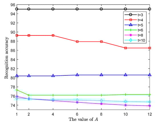
Figure 6. Effect of parameter A on classification accuracy of GHP-CNN.

The size of the initial kernel width $\sigma$ affects the coverage of pattern nodes of the GHP-CNN, thereby affecting the number of mode layer nodes. If the value of $\sigma$ is too small, then the coverage region of the generated pattern node does not contain other sample points, and the PNN classifier is close to the nearest neighbor classifier, which is equivalent to using a training sample to represent a pattern node, and the structure of the network pattern layer cannot be simplified in this case. If the value of $\sigma$ is too large, the selected pattern node cannot reflect the real sample distribution and may increase the number of heterogeneous samples in the kernel, which seriously affects the classification accuracy. In the algorithm of this paper, the input sample was a vector after the hyperspherical mapping, so that $\sigma$ could be kept in a small range for proper selection. As shown in Figure 7, when $\sigma$ was between 0.05 and 0.25, the GHP-CNN algorithm could achieve a relatively good classification accuracy.

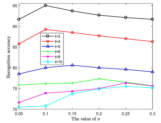
Figure 7. Effect of parameter $\sigma$ on classification accuracy of GHP-CNN.

Note that different h values lead to differences in the separability of the normalized samples. We can select h according to the following separability criterion.

$$h=\underset{h}{argmax}\left[\frac{tr\left({\mathbf{SM}}_b\right)}{tr\left({\mathbf{SM}}_t\right)}\right]$$

(10)

where ${\mathbf{SM}}_b$ and ${\mathbf{SM}}_t$ denote the between-class scatter matrix and total scatter matrix of the normalized training samples, respectively. However, as a new dimension, the value of h should be matched with the other dimensions. Therefore, the initial value of h can be selected as follows.

$$h=a{\left(\prod _{w=1}^n{\Delta }_w\right)}^{\frac{1}{n}}+(1-a){(det\left({\mathbf{SM}}_t\right))}^{\frac{1}{n}}$$

(11)

where $a\in [0,1]$. ${\displaystyle \prod _{w=1}^n}{\Delta }_w$ denotes the volume of an n-dimension hypercube for the target sample space, and det (${\mathbf{SM}}_t$) measures the volume of an n-dimension superellipsoid of the sample scatter for the target set. We compute the two volumes differently because the actual distribution shape of the features of the target set is generally irregular.

To ensure fairness in the comparison, all algorithms were tested using the same CPU. The unit of time consumed was in seconds. As shown in Table 6, the computational efficiency of the CNN-ELM and CNN-SVM algorithms was significantly higher than that of the other algorithms. The VGG-16-E algorithm took the most time because the node parameters of the MLP layer were much larger than in the other classifiers. The time required for the GHP-CNN algorithm proposed in this paper was much lower than the VGG-16-E test time.

Table 6. Comparison of test time for each algorithm.

$\mathit{s}=90$	$\mathit{t}=3$	$\mathit{t}=4$	$\mathit{t}=5$	$\mathit{t}=6$	$\mathit{t}=8$	$\mathit{t}=10$
VGG-16-E	19.15	28.36	32.42	41.51	56.84	71.91
CNN-PNN	19.21	28.31	32.93	41.33	57.72	72.64
CNN-SVM	19.01	28.02	32.02	41.03	56.03	71.04
CNN-ELM	19.00	28.00	32.00	41.00	56.04	71.08
GHP-CNN	19.25	28.22	32.69	41.28	57.58	72.45

6. Conclusions

In this paper, the generalization ability of a CFM to extract image features was studied and a novel quantization index for the CFM was defined. The analysis showed that the trained CFM could obtain abstract features with good separability. Since the distribution of the extracted features was unknown and the MLP classifier in the fully connected layer sometimes fell into a local optimum, an improved classifier named the structure-optimized probabilistic neural network (SOPNN) was used for various abstract feature classifications. Utilizing the characteristics of the CFM and the classification ability of the SOPNN, a novel generalized hybrid probability convolutional neural network (GHP-CNN) was proposed. Experiments showed that, for the same abstract features, the proposed GHP-CNN was superior to the existing hybrid neural networks in terms of classification ability.

References

- Ahonen, T.; Hadid, A.; Pietikainen, M. Face description with local binary patterns: Application to face recognition. IEEE Trans. Pattern Anal. Mach. Intell. 2006, 28, 2037–2041. [Google Scholar] [CrossRef] [PubMed]
- Satpathy, A.; Jiang, X.; Eng, H.L. LBP-based edge-texture features for object recognition. IEEE Trans. Image Process. 2014, 23, 1953–1964. [Google Scholar] [CrossRef] [PubMed]
- Bay, H.; Ess, A.; Tuytelaars, T.; Van Gool, L. Speeded-up robust features (SURF). Comput. Vis. Image Underst. 2008, 110, 346–359. [Google Scholar] [CrossRef]
- Li, J.; Zhang, Y. Learning surf cascade for fast and accurate object detection. In Proceedings of the IEEE Conference on Computer Vision and Pattern Recognition, Portland, OR, USA, 23–28 June 2013; pp. 3468–3475. [Google Scholar]
- Dellinger, F.; Delon, J.; Gousseau, Y.; Michel, J.; Tupin, F. SAR-SIFT: A SIFT-like algorithm for SAR images. IEEE Trans. Geosci. Remote Sens. 2015, 53, 453–466. [Google Scholar] [CrossRef]
- Zheng, L.; Yang, Y.; Tian, Q. SIFT meets CNN: A decade survey of instance retrieval. IEEE Trans. Pattern Anal. Mach. Intell. 2018, 40, 1224–1244. [Google Scholar] [CrossRef]
- Song, L.; Liu, J.; Qian, B.; Sun, M.; Yang, K.; Sun, M.; Abbas, S. A deep multi-modal CNN for multi-instance multi-label image classification. IEEE Trans. Image Process. 2018, 27, 6025–6038. [Google Scholar] [CrossRef]
- Ferrari, C.; Lisanti, G.; Berretti, S.; Del Bimbo, A. Investigating nuisances in DCNN-based face recognition. IEEE Trans. Image Process. 2018, 27, 5638–5651. [Google Scholar] [CrossRef]
- Yin, X.; Liu, X. Multi-task convolutional neural network for pose-invariant face recognition. IEEE Trans. Image Process. 2018, 27, 964–975. [Google Scholar] [CrossRef]
- Basu, T.; Menzer, O.; Ward, J.; SenGupta, I. A Novel Implementation of Siamese Type Neural Networks in Predicting Rare Fluctuations in Financial Time Series. Risks 2022, 10, 39. [Google Scholar] [CrossRef]
- LeCun, Y.; Bottou, L.; Bengio, Y.; Haffner, P. Gradient-based learning applied to document recognition. Proc. IEEE 1998, 86, 2278–2324. [Google Scholar] [CrossRef]
- Rama-Maneiro, E.; Vidal, J.C.; Lama, M. Embedding Graph Convolutional Networks in Recurrent Neural Networks for Predictive Monitoring. arXiv 2021, arXiv:2112.09641. [Google Scholar]
- Nassar, M.; Wang, X.; Tumer, E. Fully Convolutional Graph Neural Networks using Bipartite Graph Convolutions. ICLR 2020. [Google Scholar]
- Hong, Y.; Liu, Y.; Yang, S.; Zhang, K.; Wen, A.; Hu, J. Improving graph convolutional networks based on relation-aware attention for end-to-end relation extraction. IEEE Access 2020, 8, 51315–51323. [Google Scholar] [CrossRef]
- Krizhevsky, A.; Sutskever, I.; Hinton, G.E. Imagenet classification with deep convolutional neural networks. In Advances in Neural Information Processing Systems; MIT Press: Cambridge, MA, USA, 2012; pp. 1097–1105. [Google Scholar]
- Szegedy, C.; Liu, W.; Jia, Y.; Sermanet, P.; Reed, S.; Anguelov, D.; Erhan, D.; Vanhoucke, V.; Rabinovich, A. Going deeper with convolutions. In Proceedings of the IEEE Conference on Computer Vision and Pattern Recognition, Boston, MA, USA, 7–12 June 2015; pp. 1–9. [Google Scholar]
- Simonyan, K.; Zisserman, A. Very deep convolutional networks for large-scale image recognition. arXiv 2014, arXiv:1409.1556. [Google Scholar]
- He, K.; Zhang, X.; Ren, S.; Sun, J. Deep residual learning for image recognition. In Proceedings of the IEEE Conference on Computer Vision and Pattern Recognition, Las Vegas, NV, USA, 27–30 June 2016; pp. 770–778. [Google Scholar]
- Niu, X.X.; Suen, C.Y. A novel hybrid CNN–SVM classifier for recognizing handwritten digits. Pattern Recognit. 2012, 45, 1318–1325. [Google Scholar] [CrossRef]
- Duan, M.; Li, K.; Yang, C.; Li, K. A hybrid deep learning CNN–ELM for age and gender classification. Neurocomputing 2018, 275, 448–461. [Google Scholar] [CrossRef]
- Fu, M.y.; Liu, F.y.; Yang, Y.; Wang, M.l. Background pixels mutation detection and Hu invariant moments based traffic signs detection on autonomous vehicles. In Proceedings of the 33rd Chinese Control Conference, Nanjing, China, 28–30 July 2014; pp. 670–674. [Google Scholar]
- Pan, S.J.; Yang, Q. A survey on transfer learning. IEEE Trans. Knowl. Data Eng. 2010, 22, 1345–1359. [Google Scholar] [CrossRef]
- Blitzer, J.; Crammer, K.; Kulesza, A.; Pereira, F.; Wortman, J. Learning bounds for domain adaptation. In Advances in Neural Information Processing Systems; MIT Press: Cambridge, MA, USA, 2008; pp. 129–136. [Google Scholar]
- Liu, F.; Lin, G.; Shen, C. CRF learning with CNN features for image segmentation. Pattern Recognit. 2015, 48, 2983–2992. [Google Scholar] [CrossRef]
- Xie, G.S.; Zhang, X.Y.; Yan, S.; Liu, C.L. Hybrid CNN and dictionary-based models for scene recognition and domain adaptation. IEEE Trans. Circuits Syst. Video Technol. 2015, 27, 1263–1274. [Google Scholar] [CrossRef]
- Nguyen, D.T.; Pham, T.D.; Baek, N.R.; Park, K.R. Combining deep and handcrafted image features for presentation attack detection in face recognition systems using visible-light camera sensors. Sensors 2018, 18, 699. [Google Scholar] [CrossRef]
- Guo, Z.; Chen, Q.; Wu, G.; Xu, Y.; Shibasaki, R.; Shao, X. Village building identification based on ensemble convolutional neural networks. Sensors 2017, 17, 2487. [Google Scholar] [CrossRef] [PubMed]
- Krizhevsky, A.; Hinton, G. Learning Multiple Layers of Features from Tiny Images. Master’s Thesis, University of Toronto, Toronto, ON, Canada, 2009. [Google Scholar]
- Pei, J.; Fan, H.; Pu, L. Range space super spherical cap discriminant analysis. Neurocomputing 2017, 244, 112–122. [Google Scholar] [CrossRef]
- Wen, H.; Xie, W.; Pei, J.; Guan, L. An incremental learning algorithm for the hybrid RBF-BP network classifier. EURASIP J. Adv. Signal Process. 2016, 2016, 57. [Google Scholar] [CrossRef]
Publisher’s Note: MDPI stays neutral with regard to jurisdictional claims in published maps and institutional affiliations. |
© 2022 by the authors. Licensee MDPI, Basel, Switzerland. This article is an open access article distributed under the terms and conditions of the Creative Commons Attribution (CC BY) license (https://creativecommons.org/licenses/by/4.0/).