Abstract
The rapid development of urban industrialization has had many negative effects on the quality of water sources around cities. Long-term prediction of water quality can be of great help to the conservation of water environment. This case tries to use several popular deep learning models, such as RNN, LSTM, MLP, and Transformer-based models to predict the long-term integrated water quality index in the Chaohu Lake area. The dataset is derived from daily monitoring data from four monitoring sites within Chaohu Lake from 2019 to 2022, and the long-term prediction performance of the model is evaluated using MAE and MSE as evaluation metrics. The experimental results showed that all models selected in this case achieved good results within the study area, but Informer performed more prominently (MSE = 0.2455, MAE = 0.2449) as the length of the prediction series increased. Our results demonstrate the effectiveness of popular deep learning models in the field of WQI prediction, especially the significant advantage of transformer-based models represented by Informer in long-term water quality prediction, which will further provide an effective modern tool for water quality monitoring and management.
1. Introduction
Water is essential for human as well as natural systems and is the most critical resource for ecosystem stability and sustainable social development [1]. In particular, surface water is considered to be one of the most important ecological factors that play a role in balancing the water cycle. However, with the continuous development of industrial civilization, climate change, inappropriate human land resource utilization practices, and gross negligence in water quality management have led to further increase in surface water pollution [2,3]. Therefore, the assessment and estimation of river water quality level is a great concern today. An accurate estimation and assessment of river water quality is the basis of water environment management, which is important for the effective protection of water environment.
To make the relevant staff in water environment assessment with practical and quantitative information, Brown et al. [4] proposed WQI, the water quality index, which is calculated based on various physicochemical parameters of water (such as turbidity (TUR), total nitrogen (TN), PH and other pollutant concentrations), aiming to effectively assess the overall quality of water sources, and has been extensively used in the work related to the field of water quality. However, on the basis of its large calculation volume, the process of obtaining WQI requires a lot of time and effort of professional staff [3]. In addition, the different calculation methods of WQI also lead to an increase in workload. Therefore, improving the efficiency and estimation ability of WQI calculation exists a high practical application value [5].
At this stage of research, the comprehensive water quality index WQI prediction by time-series prediction model can effectively assess the water quality and on this basis to achieve the early detection of pollution, timely prevention, and control of water sources [6]. The good performance of deep learning in the case of large data size and the more powerful information capture ability of covariate prediction methods have attracted the attention of researchers. Emamgholizadeh et al. [7] used Multilayer Perceptron (MLP), Convolutional Neural Network (CNN) for water quality components during the study of Karoon River water quality, and pointed out that all the applied models have suitable performances in water quality prediction, among which MLP has slightly higher prediction accuracy in all contexts, but it is not difficult to find in the final results that these methods, although improved over previous ones, are still deficient in capturing long-term dependence. Later, Beak et al. [8] created a new deep learning method by using long short-term memory (LSTM) to conduct a study in the Nakong River basin in Korea, simulating a variety of parameter variables affecting water quality conditions in the process. LSTM itself solves the problems of gradient disappearance and gradient explosion that exist in RNN-like methods when the network is deepened [9]. Such improvements significantly improve the utilization of data and the accuracy of predictions of regional water quality. However, it is still weak in capturing long-term dependence [10], and its mastery of auxiliary variables as one of the models for covariate forecasting still needs to be improved.
With the continuous development in the field of deep learning coupled with time series prediction, Long Sequence Time-Series Forecasting (LSTF) has gradually started to be noticed by researchers. Compared with short time-series prediction, LSTF is closer to realistic scenarios [11], it can effectively capture the more accurate long-range correlation coupling between output and input, and this kind of prediction can provide us with timely warning of pollution criticality [12] and thus maintain the ecological environment. balance. Therefore, LSTF is more suitable for realistic fields like water quality prediction assessment, so this paper combines the above-mentioned classical deep learning models: MLP, RNN, Transformer, and LSTM with the field of long-range time series prediction, and explores the prediction ability of these models on LSTF problems while comparing with the long-term time series prediction models FEDformer [13] and Informer [14] for a comparison of each prediction performance.
In this case study, we have made three main contributions aimed at providing corresponding assistance to subsequent researchers in the field of water quality:
- For the particular study area of Chaohu Lake, the variables affecting the water quality index WQI are grouped to find the best prediction effect and the corresponding weighting proportion.
- The perspective of the field of water quality forecasting from short sequence to the new field of long sequence time-series forecasting proved that LSTF has more excellent control ability in the relationship between multiple variables, and LSTF can solve the actual long-term water quality forecasting problem, proved the degree of suitability of long series forecasting and water quality forecasting.
- Compare the prediction results of LSTF model informer and several popular deep learning models for long sequence, find out the best long sequence forecasting model under one specific field of water quality prediction, and provide effective modern prediction tools and tools for water quality prediction.
2. Study Area
Chaohu Lake (31°42∼32°25 N, 116°23∼118°22 E) is one of the five major freshwater lakes in China in the middle and lower reaches of the Yangtze River. It is located in central Anhui Province, China, with a perimeter of 176 km, an average depth of 2.89 m, an area of 780 km, and a volume of 2.07 billion m [15]. The lake is mainly recharged by surface runoff, with a watershed area of 13,486 km and 35 rivers along the lake [16]. Chaohu Lake has a northern subtropical temperate monsoon climate with significant monsoons and four distinct seasons. The average annual temperature of the entire basin is between 15 and 16 °C, the active cumulative temperature is above 4500 °C, the frost-free period is above 200 days, the annual temperature difference is above 25 °C, and the annual precipitation contour of 1000 mm passes through the district boundary [17]. The main roles of the basin are shipping, water supply, irrigation, aquaculture, tourism, and many other functions. Figure 1 illustrates the land use pattern of the Chaohu Lake watershed, with urban land (red blocks) dominating the upstream, while the peripheral areas of the watershed are dominated by paddy fields for cultivation and aquaculture, while the downstream is dominated by scattered industrial and other special land uses [15,18].
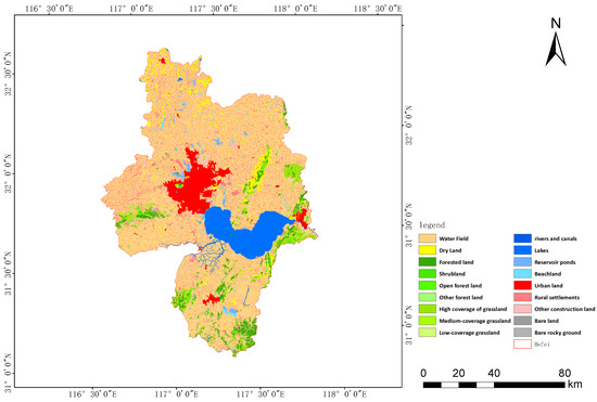
Figure 1.
Distribution of utilization types in the Chaohu Lake watershed.
In a study published by Zhang et al. [19] in 2022, it was noted that the annual average amounts of total nitrogen and total phosphorus in the basin were estimated to be 10,832 t/a and 781 t/a. This case study also shows that the load intensity within the watershed is unevenly distributed, and soil erosion, precipitation intensity, and population density, as the three key factors driving N and P losses, show a positive correlation with the intensity of N and P losses. In addition, the studies by He et al. and Ren et al. [20,21] both showed that the water quality pollution of Chaohu Lake mainly originated from the rapid population growth and economic development, and the high-intensity human activities further deteriorated the water quality. Untreated domestic sewage, industrial wastewater, and massive application of pesticides in major tributaries, all of which have caused accumulation of nutrients in their water bodies, increased net primary productivity, increased eutrophication, shrinking of lakeshore ecological zones, elevated lake bottoms and accelerated aging of the lakes. It is extremely important to establish a water quality prediction model that meets the long-term needs to cope with the changing trends in the future stages [22].
The data for this study was selected from some monitoring sections in the Chaohu basin, which are located at the latitude and longitude as shown in Table 1. By analyzing the geographic environment of the monitoring points on the map, including relative location, topography, climate, vegetation, soil, and distribution in the upstream and downstream of the basin, three more representative monitoring sections in Figure 2: Lakeside, Chaohu Shipyard, and the Zhaojia River intake area were chosen as cases for this study to implement the proposed model.

Table 1.
Longitude and latitude distribution of Chaohu water quality monitoring section.

Figure 2.
Distribution of water quality monitoring section points in Chaohu Lake.
3. Data and Methods
3.1. Data Collection and Processing
In 2019, Anhui Province released The Chaohu Lake Basin Water Pollution Management Regulations, which will be officially implemented in 2020. In response to this policy, we selected the water quality monitoring data of Chaohu Lake from 2019 to 2022 for predictive modeling to ensure that the model matches the current stage of water quality, while aiming to provide a modern tool for water quality prediction in Chaohu Lake and to provide assistance for subsequent studies. Daily water quality data have been collected from the Chaohu Lake basin between 2019–2022 were obtained from the water quality monitoring reports provided in the 2022 summary by the China Environmental Quality Monitoring Bureau, which includes ten variables relevant to WQI calculations [23]: water temperature (°C), pH, , turbidity (TUR), dissolved oxygen (DO), total nitrogen (TN), ammonia nitrogen (-N), nitrite (-N), total phosphorus (TP), nitrate nitrogen (-N). Sampling, preservation, storage, and analysis procedures followed national surface water monitoring guidelines.
With reference to the water quality parameters that have been collected and a number of current related studies, the integrated water quality index method proposed by PESCE and EUNDERLIN [23] was chosen to calculate the WQI by nine parameters, and the formula for WQI is expressed as follows:
In the above equation, i is the total number of parameters included in the study; is the normalized value of parameter i (Table 2); is the weight assigned to the water quality parameter according to its effect on primary health perception (Table 3), the maximum weight of the parameters known to affect water quality is 4 and the minimum is 1. The accuracy of these parameter values have been verified in several studies [24,25], and which is calculated on this basis by the above equation, is the integrated water quality parameter WQI that we need afterward.
Table 2.
WQI calculation table.
Table 3.
Chaohu WQI.
As visible in Table 3, the calculated WQI ranges from 0 to 100, and the better value symbolizes the better water quality situation According to the WQI score, the water quality is divided into five different levels: I Excellent (90–100 points), II Good (71–90), III Medium (51–70), IV Average (26–50), and V Poor (0–25) [26].
Under the guidance of the above method, the water quality parameters collected from the selected monitoring segments in the Chaohu Lake basin were analyzed and processed to obtain the descriptive statistics of the WQI variables as shown in Table 4 and to calculate the WQI for the corresponding time periods. In addition, the calculated WQI shows that the overall water quality situation in the Chaohu Lake basin varies widely, with specific values ranging from good excellent (WQI = 85) to average quality (WQI = 46) varying.
Table 4.
Daily monitoring data of water quality variables in Chaohu Lake and descriptive statistics of WQI during 2019–2022.
The water quality variable monitoring data collected in this case study were daily water quality from 2020 to 2022, totaling 40,400 items, and were divided into two datasets [27]: 75 percent of the data will be used for the training process of the model and 25 percent for the testing process. This classification method, which is widely used in such data-driven modeling as time-series prediction, was able to achieve relatively good Experimental results [5,27].
3.2. Predictive Models for Deep Learning
Focusing on the specific field of water quality, this paper chooses the long sequence time series forecasting method (LSTF) which is closer to the real situation to predict the selected water quality parameter WQI. In the model, we compare the deep learning models such as MLP, RNN, LSTM, Transformer, etc., which are often used in short sequence time series forecasting research, and the newly proposed Informer and FEDformer models in the field of LSTF in recent stage. Exploring their ability in solving the specific LSTF problem of water quality forecasting, the following is a comparison of LSTF and the Informer model, with the best benefits, are presented.
3.2.1. Long Sequence Time Series Forecasting
In many practical applications, we need predictions for long series time series, such as sensor network monitoring [28], stock price trends [29], and water quality forecasting. As explored in this paper, such predictions can provide us with timely warning of pollution thresholds and thus maintain ecological balance, which is important for social and ecological development. LSTF is closer to realistic scenarios than short-term predictions because a large number of time series of past behaviors are needed to support in its predictions. This also reflects the need for LSTF models to have high computational predictive power, that is, to effectively capture more accurate long-range correlations between outputs and inputs. The results in Figure 3a, similarly, shows that, as Zhou et al. [14] states, the LSTF can extend beyond the short-range prediction limit for predicted sequences after training, and longer than short-range time-series predictions.
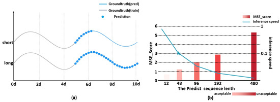
Figure 3.
(a) Comparison of the limit sequence lengths that can be predicted by LSTF and SSTF. (b) Prediction length and accuracy of prediction results.
However, LSTF does not perform as well as we expected due to the limitations of the predictive model at this stage. Despite the fact that it has better coverage and can be better used as a forecasting tool for planning and implementation, few people choose to use it. We can see that Figure 3b shows the MSE scores of models such as RNN, MLP, LSTM, and Transformer. These models are usually used for short-term prediction, and when the prediction type changes from short-term to long-term, the MSE scores of these models increase with the growth of the prediction sequence, while the inference speed decreases significantly. Therefore, when the prediction type changes from short-term to long-term and the length of the input sequence reaches 48, the MSE loss of the corresponding model is no longer acceptable [14] and is not suitable for solving the problem of LSTF class with long sequence of inputs.
3.2.2. Informer
At this stage, Transformer models are constantly applied in various fields of deep learning, and they all show very good performance. In the field of temporal prediction, Transformer shows its profound potential in capturing long-range dependencies [14], which shows a new possibility to solve the above-mentioned problems faced by LSTF. After this, a large number of experimental studies have shown that there is extremely good compatibility between the intrinsic properties of the Transformer and the LSTF, but the Transformer model alone suffers from three major problems [30]: high quadratic computational complexity of self-attention; memory bottleneck of stacked layers under long sequence inputs and slow inference speed when predicting long sequence outputs. Therefore, the original Transformer model is not suitable for direct use in solving problems in LSTF. Therefore, in order to effectively utilize Transformer’s grasp of long sequence features and apply it to LSTF, Zhou’s team [14] modified the structure of the original Transformer and proposed an improved long sequence time-series prediction model, Informer. They verified the potential value of the model during testing, Transformer’s ability to capture individual long-term correlations between the output and input of long sequence time sequences. In addition, in the structure of the model Informer proposed improvements for the three major defects faced by Transformer in solving the LSTF problem, respectively, as follows Figure 4 shows the general architecture of Informer proposed by zhou’s team [14].

Figure 4.
The overall architecture of Informer.
The first is the quadratic computational property of self-attention. The dot product operation of Mechanism makes the time complexity and space complexity of each layer O, which makes the computational processing time of the model rise significantly with the increase of the length of the prediction sequence, and is not suitable for LSTF. In contrast, subsequent work has shown that the distribution of Self-Attention Probability is sparse; in fact, only a few dot product pairs contribute most of the attention, while the rest is negligible and obeys a long-tailed distribution. Based on such results, Informer proposed ProbSparse self-attention based on the original one, which reduces the spatio-temporal complexity from O to O(LlogL)
Among them, Q is the query vector, K is the key vector, V is the value vector, and d is the number of columns of the Q, K matrix which is the dimension of the vector. ProbSparse self-Attention enables the model to have higher arithmetic power when solving the LSTF problem in dealing with a long sequence of inputs, and at the same time its sampling result is the same for each head when sampling the key randomly for each query, that is, the sampled key is the same. But since each layer of self-attention first does a linear transformation of Q, K, and V, this makes the query and key vectors corresponding to different heads at the same position in the different sequence, i.e., each head takes a different optimization strategy. Each head is stitched together and the final output matrix is obtained by fusion as follows:
Moreover, Informer proposes the Self-Attention Distilling operation permission to control the attention scores in J-Stacking Layers for the memory bottleneck of the Transformer, which reduces the memory usage of J stacking layers. In order to enhance the robustness of distillation operations, the encoder architecture of informer also builds multiple encoder stacks, gradually reducing one distillation operation layer and half of the input length at a time, and finally stitching all the stack outputs together, using self-attention distillation operations to reduce the redundancy generated in the attention results and refine the main attention, reducing the total memory usage from O to O(), which also leads to a more scalable model when receiving long sequence inputs. At the same time, the dynamic decoding operation of the original Transformer makes dynamic decoding (step-by-step inference) worse than other prediction models, and the speed drop is more obvious in the case of long-term prediction, so Informer proposes the Generative Style Decoder. Using a standard decoder structure consisting of a stack of two identical multi-head attention layer, generative inference can effectively mitigate the speed drop in the long-term prediction problem by feeding the following vectors into the decode:
where start token is the known sequence before the target sequence and is the timestamp sequence of the target sequence. Compared with the original decoding method, generative inference enables the model to obtain all the predicted data in just one forward step by changing the original decoding method, so that the model only needs one forward step to get all of the predicted data and decode all elements at once, which is more efficient than dynamic decoding.
In addition, not only local timing information but also hierarchical and agnostic timestamps are required in the input of LSTF problems. It is difficult to adapt directly to the conventional self-attentive mechanism, and the query-key mismatch between the encoder and decoder degrades the prediction performance. The embedding of the input consists of three independent parts.
- Local timestamp. The contextual information is preserved by a fixed location embedding, the location encoding of the original Transformer:Among them
- Global timestamps. The global timestamp is represented by a learnable stamp embedding with a restricted vocabulary (up to 60, at the finest granularity per minute). That is, the self-focused similarity computation has access to the global context and the computational consumption is tolerable of long inputs.
- Alignment dimensionality. The scalar context is mapped to the dmodel dimensional vector using a one-dimensional convolutional filter (width 3, step 1).
Finally, by using the above three steps, the sequence of feed-in models can be obtained
In the above equation, , is a factor that balances the size between the scalar mapping and the local/global embedding, and if the sequence input is normalized, then = 1.
3.3. Building Deep Learning Forecasting Models
In the process of model construction, the selection of data is required to ensure that there are a sufficient number of variables and that these variables have a sufficient information base to support the first important step of predicting WQI. At the same time, ensuring a sufficient amount of information and a sufficient base of information can effectively avoid adverse effects on the prediction performance and improve the accuracy of the model. Nine WQI variables were identified as potential inputs.
According to Table 5, which shows the weights assigned to each water quality parameter in the Chaohu basin under the influence of primary health perception [24,25], we can find that DO has the largest weight, followed by , COD, TN, TUR, TP, and T. It is worth mentioning that here we selected the parameters that were assigned weights in the test basin under primary health perception, taking into account the fact that Chaohu Lake is mainly polluted by agriculture and industry. The parameters that were given weights were grouped into combinations from large to small (Table 6), and a “trial-and-error” approach was used to determine the combination of parameters that gave the best fit to the prediction models [31]. These models were evaluated during the testing process. In this study, three libraries (python-based packages), sci-kit learn, torch, and NumPy, were used to develop a temporal prediction model for predicting WQI.
Table 5.
Weight assignment of each water quality parameter.
Table 6.
Grouping of water quality variables based on assigned weights S1–S10.
3.4. Performance Evaluation of Deep Learning Prediction Models
Mean absolute error (MAE) and mean square error (MSE) was applied in this model to evaluate the statistical values of the efficiency of the two models to indicate the degree of fit between the predicted and actual values. The MAE was used to show the deviation between the actual and predicted values, and the MSE was used to measure the degree of similarity between the two medium data [32].
In the above equation, n is the total number of predicted values, is the observed value, O is the average of the observed values, is the predicted value
4. Results and Discussion
4.1. Forecasting Performance Analysis of Deep Learning Models Based on 10 Classifications
In forecasting the Chaohu WQI, we set 10 different combinations of expected relevant feature variables based on the corresponding weights. In addition, we used six different deep learning models for covariate prediction based on different groupings, and MAE and MSE were used as two different metrics to evaluate the performance of the prediction models. The experimental results for all models and variable groupings are recorded in Table 7. In total, 10 × 6 = 60 different cases of predictive ability of the corresponding models. Among the many prediction options, combining the two different performance parameters, Informer-S8 shows the best prediction performance in solving LSTF problems like water quality prediction: MSE = 0.2455 and MAE = 0.2449. In addition, compared with other classical models for short-term time series prediction, the newly proposed LSTF models: FEDformer and Informer, when dealing with problems like water quality prediction plus long series input, do have the corresponding prediction accuracy and have achieved better fitting results in various variable classifications.
Table 7.
Efficiency statistics of 6 DL models for 10 combinations of input variables during testing.
4.2. The Performance of Popular Models in the Field of Short-Term Prediction on LSTF
Among the models selected in this case study, by comparing each classical model commonly used for short-term time series prediction except Informer and FEDformeer, it can be found that Figure 5 shows MLP-S10 (MSE = 0.3319, MAE = 0.3523), LSTM-S10 (MSE = 0.5914, MAE = 0.6041), RNN-S9 (MSE = 0.5794, MAE = 0.5963), and Transformer-S7 (MSE = 0.3122, MAE = 0.4432) achieve the best prediction results in their respective domains. The MLP-S10 performs the best among these, with the lowest values of both MSE and MAE among many model groups, the best fitting the MSE and MAE of MLP-S10 have the lowest value, i.e., the best fit, among many model-groups. However, it is not difficult to see that the classical Deep Learning model often used in short-term prediction in solving the LSTF class water quality prediction problem, the accuracy of prediction, which shows a positive ratio with the number of input feature variables, in general, increases as the number of input variables increases. Although, the grouping with the highest prediction accuracy is not necessarily the one with the highest number of variables, in general, the group with the best prediction must have an accumulation of the number of variables. It is easy to see from Figure 6, such models in the face of water quality prediction problem, as the type of input feature variables continue to reduce, the actual—prediction of the goodness-of-fit also decreases continuously. In addition, in the face of long series of inputs, the prediction model’s ability to grasp the features also decreases as the length increases. Overall, the prediction effect of such models are highly volatile, and the performance is not as good as that of LSTF-type models, so it is not suitable for solving this type of problem for long sequence input plus water quality prediction for the case.
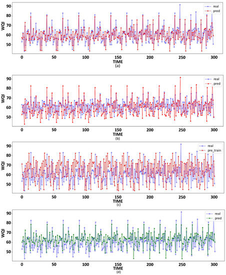
Figure 5.
The best performance model for the corresponding algorithm during the test period observes and predicts the temporal variation of the WQI values: (a) MLP-S10 (b) LSTM-S10 (c) RNN-S9 (d) Transformer-S7.
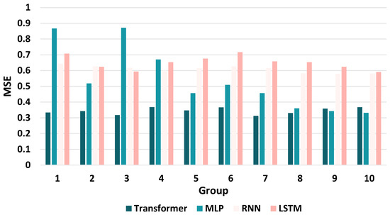
Figure 6.
Changes in MSE of the model in different variable groupings.
In addition, it is clear from what Figure 5 shows us that the model, which is used for short-term forecasting, is better in the case of smooth fluctuations when facing the LSTF problem. However, in the case of large fluctuations, the fit is poor, and the degree of control over the hidden laws of the predictor variables was lacking, which, in reality, means relatively weak control over seasonal patterns and cyclical changes. The characteristics of LSTF can make up for this deficiency, which shows us that LSTF has excellent adaptability and trial value in this field. This also directs our attention to the use of the LSTF, which is closer to real life, to solve related problems.
4.3. Performance of LSTF Models in Long Sequence Time Series Forecasting Species
Informer and FEDformer, which were proposed as models to solve the LSTF problem, did show different degrees of accuracy than the other four classical short-term time-series forecasting research models when solving the water quality forecasting plus long sequence input problem. Figure 7 shows both Informer-S8 (MSE = 0.2455, MAE = 0.2449) and FEDformer-S9 (MSE = 0.3867, MAE = 0.4919) achieved better performance assessments than the other models. The data summarized in Table 7 above are plotted as MSE (Figure 3a) and MAE (Figure 8b) from S1 to S10 by different models to obtain Figure 8. According to the undulating condition of the Figure 8, Informer and FEDformer, a class of LSTF models, have good and stable forecasting effects in the context of long sequence forecasting with different feature inputs, and compared with other models, it has better adaptability and closer to the realistic environment.

Figure 7.
Observed and predicted time variation of WQI values using the best performance model based on the LSTF algorithm during the test period: (a) Informer-S8 (b) FEDformer-S9.

Figure 8.
Changes in MSE of the model in different variable groupings: (a) MSE loss (b) MAE loss.
Informer is the best model among the 6 deep learning models in the field of long-term water quality prediction of Chaohu Lake, and the histogram of the performance index of each model at the best performance grouping by Figure 8 shows that Informer is much better than the other 5 time-series prediction models in the prediction of long-term water quality index WQI. And in Figure 8 of the forecast loss graph for each group of Informer, we can see that Informer has a high degree of confidence in the long series input, and measures the low volatility of the forecast loss values for different groupings.
4.4. Discussion
There are six Deep Learning models in this comparison, and, in general, they are divided into two categories: classical models for short-term forecasting, RNN, LSTM, MLP, Transformer, and long sequence time series forecasting models, Informer, and FEDformer. The performance parameters of each model in solving LSTF water quality WQI forecasts for a specific study area was experimentally measured, and we found that all models have excellent forecasting ability, and among them, the LSTF models are basically better than other models, and Informer is the most excellent forecasting model. In addition, we found that different prediction models have different groups of feature variables for the best prediction results in solving LSTF problems, which also proves that DL models do not have the same effect when facing different combinations of feature variables as inputs. The MLP and LSTM have the best prediction performance in the case of S10, while FEDformer and RNN have the best results in the case of S9, while Informer and Transformer have the highest prediction accuracy in the cases of S8 and S7, respectively.
Based on the field of water quality prediction, Informer has a better prediction performance than fedformer and other models, and its accuracy and seasonal grasp of the actual application area have good performance; for the prediction area, water quality prediction and water quality assessment will be affected by the local natural environment and has its own regional characteristics, so in a particular environment, the best performance of the Deep Learning time series prediction model will also change. In other studies, Zhou’s team [33] chose the LSTM model for the comparison of two different regions, Lake Tai and Lake Victoria, and it was the model with the highest prediction accuracy. In the study, and similarly, in the case study of Poyang Lake basin by He’s team [22], the VCLM outperformed the LSTM model and achieved a better performance. After that, in Khoi’s [34] water quality prediction study of Labuan River, it shows us that most models change in the face of different regional models by comparing them with 12 different ML models. Therefore, the optimal prediction model in a specific study area may not necessarily be able to achieve the migration of other regions, so the water quality prediction assessment model with regional generality is still the main core of exploration now.
An important factor affecting the prediction effect between the same prediction model is the consideration of cross-influence between variables, placed in the prediction of water quality composite index, WQI, in addition to the characteristic parameters of water quality testing hydrological characteristics (such as flow rate, icing period, and sand content) land use class, land use classification and climate (temperature, precipitation) and other factors of the composite impact. Although these parameters cannot directly affect the water quality, in time series prediction, the more features are considered and the more interrelationships are set, which can help our predictions to be closer to the real environment. This will also give the opportunity for deep learning prediction models to have higher accuracy and provide more modern tools for subsequent research.
5. Conclusions
In this case study, by assigning different weights to the variables affecting the comprehensive water quality index, WQI, according to their strength of influence, and conducting experiments with 10 different groupings respectively, it was demonstrated that in the process of long sequence time series forecasting, the corresponding optimal variable groupings are not the same for different Deep Learning models. Therefore, in the process of water quality prediction, adjusting the variables involved in the prediction is also an important part of the model performance, and through comparative experiments, this paper provides the best combination of variables relative to this one specific area of Chaohu Lake to provide guidance for subsequent research.
After that, we shift the water quality forecasting from short sequence to long sequence time series forecasting. In the selection of models, we chose six different deep learning models including four classical models RNN, LSTM, MLP, and Transformer in the field of short-term forecasting, and two newly proposed long-term forecasting models Informer and FEDformer. The prediction effectiveness of each model is evaluated by two different performance evaluation parameters, MSE and MAE, in order to select the most suitable model for long-term water quality forecasting and the corresponding grouping of variables. By comparing the actual-predicted value of the degree of fit that is MSE and MAE two major measurement parameters to select the prediction model with the highest accuracy in predicting the composite water quality index WQI. Combining LSTF and water quality prediction field, we can easily see that it can extend to the time prediction limit is more long-term, the stronger the grasp of the relationship between variables, its stronger ability to sense in advance is more suitable for the practical application of the field and the prevention of the development.
In terms of results, by comparing the degree of fit of the actual-predicted values in Table 7, i.e., the two main measurement parameters MSE and MAE, it is easy to see that Informer is ahead of other models in terms of prediction performance when solving the practical problem of water quality prediction domain + long time series input, and also has better performance than other models in the face of different sets of variables, while Informer -S8 is the best prediction case among them (MSE = 0.2455, MAE = 0.2449). In solving the LSTF Chaohu Lake water quality prediction problem, the model effect Informer > FEDformer > MLP > Transformer > RNN > LSTM, so in this particular area of long-term water quality prediction, Informer has a better adaptability and use prospects, can improve the accuracy of WQI prediction, which is conducive to better management to improve Water quality, effective pollution prevention.
Author Contributions
Conceptualization, Y.Z. (Yongheng Zhang); data curation, P.W. and Z.X.; formal analysis, Z.X.; funding acquisition, Y.W. and Y.Z. (Youhua Zhang); methodology, S.Y.; resources, Y.W. and Y.Z. (Youhua Zhang); software, P.W.; supervision, Y.Z. (Yongheng Zhang) and Z.X.; validation, S.Y. and Y.Z. (Yongheng Zhang).; writing—original draft, S.Y.; writing—review and editing, S.Y. and Z.X. All authors have read and agreed to the published version of the manuscript.
Funding
This research was funded by Anhui agricultural ecological and environmental protection and quality safety industrial technology system grant number 22803029.
Institutional Review Board Statement
Not applicable.
Informed Consent Statement
Not applicable.
Data Availability Statement
Not applicable.
Acknowledgments
We would like to thank the Beidou Precision Agricultural Information Engineering Laboratory of Anhui Province for supporting us to complete this research. And we sincerely thank Hao Wu from University of Science and Technology of China for his valuable suggestions.
Conflicts of Interest
The authors declare no conflict of interest.
References
- Ni, X.; Wu, Y.; Wu, J.; Lu, J.; Wilson, P.C. Scenario analysis for sustainable development of Chongming Island: Water resources sustainability. Sci. Total Environ. 2012, 439, 129–135. [Google Scholar] [CrossRef] [PubMed]
- Asadollah, S.B.H.S.; Sharafati, A.; Motta, D.; Yaseen, Z.M. River water quality index prediction and uncertainty analysis: A comparative study of machine learning models. J. Environ. Chem. Eng. 2021, 9, 104599. [Google Scholar]
- Singha, S.; Pasupuleti, S.; Singha, S.S.; Singh, R.; Kumar, S. Prediction of groundwater quality using efficient machine learning technique. Chemosphere 2021, 276, 130265. [Google Scholar] [CrossRef] [PubMed]
- Brown, R.M.; McClelland, N.I.; Deininger, R.A.; O’Connor, M.F. A water quality index—Crashing the psychological barrier. In Indicators of Environmental Quality; Springer: Berlin/Heidelberg, Germany, 1972; pp. 173–182. [Google Scholar]
- Bui, D.T.; Khosravi, K.; Tiefenbacher, J.; Nguyen, H.; Kazakis, N. Improving prediction of water quality indices using novel hybrid machine-learning algorithms. Sci. Total Environ. 2020, 721, 137612. [Google Scholar]
- Hmoud Al-Adhaileh, M.; Waselallah Alsaade, F. Modelling and prediction of water quality by using artificial intelligence. Sustainability 2021, 13, 4259. [Google Scholar] [CrossRef]
- Emamgholizadeh, S.; Kashi, H.; Marofpoor, I.; Zalaghi, E. Prediction of water quality parameters of Karoon River (Iran) by artificial intelligence-based models. Int. J. Environ. Sci. Technol. 2014, 11, 645–656. [Google Scholar] [CrossRef]
- Baek, S.S.; Pyo, J.; Chun, J.A. Prediction of water level and water quality using a CNN-LSTM combined deep learning approach. Water 2020, 12, 3399. [Google Scholar]
- Greff, K.; Srivastava, R.K.; Koutník, J.; Steunebrink, B.R.; Schmidhuber, J. LSTM: A search space odyssey. IEEE Trans. Neural Netw. Learn. Syst. 2016, 28, 2222–2232. [Google Scholar] [CrossRef]
- Lai, G.; Chang, W.C.; Yang, Y.; Liu, H. Modeling long-and short-term temporal patterns with deep neural networks. In Proceedings of the 41st International ACM SIGIR Conference on Research & Development in Information Retrieval, Ann Arbor, MI, USA, 8–12 July 2018; pp. 95–104. [Google Scholar]
- Maaliw, R.R.; Ballera, M.A.; Mabunga, Z.P.; Mahusay, A.T.; Dejelo, D.A.; Seño, M.P. An ensemble machine learning approach for time series forecasting of COVID-19 cases. In Proceedings of the 2021 IEEE 12th Annual Information Technology, Electronics and Mobile Communication Conference (IEMCON), Vancouver, BC, Canada, 27–30 October 2021; pp. 633–640. [Google Scholar]
- Wang, J.; Li, H.; Lu, H. Application of a novel early warning system based on fuzzy time series in urban air quality forecasting in China. Appl. Soft Comput. 2018, 71, 783–799. [Google Scholar] [CrossRef]
- Zhou, T.; Ma, Z.; Wen, Q.; Wang, X.; Sun, L.; Jin, R. FEDformer: Frequency enhanced decomposed transformer for long-term series forecasting. arXiv 2022, arXiv:2201.12740. [Google Scholar]
- Zhou, H.; Zhang, S.; Peng, J.; Zhang, S.; Li, J.; Xiong, H.; Zhang, W. Informer: Beyond efficient transformer for long sequence time-series forecasting. In Proceedings of the AAAI Conference on Artificial Intelligence, Virtual, 2–9 February 2021; Volume 35, pp. 11106–11115. [Google Scholar]
- Huang, J.; Zhan, J.; Yan, H.; Wu, F.; Deng, X. Evaluation of the impacts of land use on water quality: A case study in the Chaohu Lake Basin. Sci. World J. 2013, 2013, 329187. [Google Scholar]
- Wu, Z.; Lai, X.; Li, K. Water quality assessment of rivers in Lake Chaohu Basin (China) using water quality index. Ecol. Indic. 2021, 121, 107021. [Google Scholar] [CrossRef]
- Min, M.; Duan, X.; Yan, W.; Miao, C. Quantitative simulation of the relationships between cultivated land-use patterns and non-point source pollutant loads at a township scale in Chaohu Lake Basin, China. Catena 2022, 208, 105776. [Google Scholar] [CrossRef]
- Tang, W.; Shan, B.; Zhang, H.; Mao, Z. Heavy metal sources and associated risk in response to agricultural intensification in the estuarine sediments of Chaohu Lake Valley, East China. J. Hazard. Mater. 2010, 176, 945–951. [Google Scholar] [PubMed]
- Zhang, J.; Gao, J.; Zhu, Q.; Qian, R.; Zhang, Q.; Huang, J. Coupling mountain and lowland watershed models to characterize nutrient loading: An eight-year investigation in Lake Chaohu Basin. J. Hydrol. 2022, 612, 128258. [Google Scholar]
- He, Y.; Wang, Q.; He, W.; Xu, F. The occurrence, composition and partitioning of phthalate esters (PAEs) in the water-suspended particulate matter (SPM) system of Lake Chaohu, China. Sci. Total Environ. 2019, 661, 285–293. [Google Scholar] [CrossRef]
- Ren, C.; Wu, Y.; Zhang, S.; Wu, L.L.; Liang, X.G.; Chen, T.H.; Zhu, C.Z.; Sojinu, S.O.; Wang, J.Z. PAHs in sediment cores at main river estuaries of Chaohu Lake: Implication for the change of local anthropogenic activities. Environ. Sci. Pollut. Res. 2015, 22, 1687–1696. [Google Scholar]
- He, M.; Wu, S.; Huang, B.; Kang, C.; Gui, F. Prediction of Total Nitrogen and Phosphorus in Surface Water by Deep Learning Methods Based on Multi-Scale Feature Extraction. Water 2022, 14, 1643. [Google Scholar] [CrossRef]
- Pesce, S.F.; Wunderlin, D.A. Use of water quality indices to verify the impact of Córdoba City (Argentina) on Suquia River. Water Res. 2000, 34, 2915–2926. [Google Scholar] [CrossRef]
- Kocer, M.A.T.; Sevgili, H. Parameters selection for water quality index in the assessment of the environmental impacts of land-based trout farms. Ecol. Indic. 2014, 36, 672–681. [Google Scholar]
- Debels, P.; Figueroa, R.; Urrutia, R.; Barra, R.; Niell, X. Evaluation of water quality in the Chillán River (Central Chile) using physicochemical parameters and a modified water quality index. Environ. Monit. Assess. 2005, 110, 301–322. [Google Scholar] [PubMed]
- Jonnalagadda, S.; Mhere, G. Water quality of the Odzi River in the eastern highlands of Zimbabwe. Water Res. 2001, 35, 2371–2376. [Google Scholar] [PubMed]
- Nouraki, A.; Alavi, M.; Golabi, M.; Albaji, M. Prediction of water quality parameters using machine learning models: A case study of the Karun River, Iran. Environ. Sci. Pollut. Res. 2021, 28, 57060–57072. [Google Scholar]
- Papadimitriou, S.; Yu, P. Optimal multi-scale patterns in time series streams. In Proceedings of the 2006 ACM SIGMOD International Conference on Management of Data, Chicago, IL, USA, 27–29 June 2006; pp. 647–658. [Google Scholar]
- Zhu, Y.; Shasha, D. Statstream: Statistical monitoring of thousands of data streams in real time. In Proceedings of the 28th International Conference on Very Large Databases, Hong Kong, China, 20–23 August 2002; Elsevier: Amsterdam, The Netherlands, 2002; pp. 358–369. [Google Scholar]
- Vaswani, A.; Shazeer, N.; Parmar, N.; Uszkoreit, J.; Jones, L.; Gomez, A.N.; Kaiser, Ł.; Polosukhin, I. Attention is all you need. In Proceedings of the Advances in Neural Information Processing Systems, Long Beach, CA, USA, 4–9 December 2017; Volume 30. [Google Scholar]
- Gao, S.; Huang, Y.; Zhang, S.; Han, J.; Wang, G.; Zhang, M.; Lin, Q. Short-term runoff prediction with GRU and LSTM networks without requiring time step optimization during sample generation. J. Hydrol. 2020, 589, 125188. [Google Scholar]
- Ahmed, U.; Mumtaz, R.; Anwar, H.; Shah, A.A.; Irfan, R.; García-Nieto, J. Efficient water quality prediction using supervised machine learning. Water 2019, 11, 2210. [Google Scholar]
- Zhou, J.; Wang, Y.; Xiao, F.; Wang, Y.; Sun, L. Water quality prediction method based on IGRA and LSTM. Water 2018, 10, 1148. [Google Scholar] [CrossRef]
- Khoi, D.N.; Quan, N.T.; Linh, D.Q.; Nhi, P.T.T.; Thuy, N.T.D. Using Machine Learning Models for Predicting the Water Quality Index in the La Buong River, Vietnam. Water 2022, 14, 1552. [Google Scholar] [CrossRef]
Publisher’s Note: MDPI stays neutral with regard to jurisdictional claims in published maps and institutional affiliations. |
© 2022 by the authors. Licensee MDPI, Basel, Switzerland. This article is an open access article distributed under the terms and conditions of the Creative Commons Attribution (CC BY) license (https://creativecommons.org/licenses/by/4.0/).