4.2. Model Fitting
Classification algorithms are supervised learning methods that are widely used to solve predictive modeling problems when the response variable is labeled into classes or categories. Since the response variable considered is dichotomous, this is a binary classification problem (Collision: “1”; Avoidance:”0”).
The accuracy and performance metrics for each of these methods have been calculated using the k-fold cross-validation technique [
38], which allows different partitions of data to be selected between the training set and test set, thus ensuring the generation of independent data partitions. By using a total of k = 5 iterations, the possible overfitting derived from a small training data size is avoided, thus obtaining a higher reproducibility in the whole sample and higher reliability in obtaining the accuracy through the arithmetic mean of all k repetitions.
To obtain the hyperparameters that optimize the overall performance of the models, the GridSearchCV function of the sklearnmodel_selection module is used.
Table 7 lists these hyperparameters, which will be described in the following paragraphs.
The distance-based models are:
(1)
Support Vector Machine (SVM): This method is based on the construction of a hyperplane or set of hyperplanes in a space of very high (or even infinite) dimensionality to achieve a good separation of classes to obtain a good classification. Therefore, the greater the distance of the hyperplane to the training data points that are closest to each other, the smaller the error made by the classifier [
39].
The mathematical functions used in the SVM algorithm, known as Kernel functions, can be linear, polynomial, radial basis function (RBF), sigmoid, etc. These functions assign the data to a different, generally higher dimensional space, intending to separate the classes more simply once the transformation has been carried out and thus simplifying the complex and non-linear decision limits to make them linear in the primitive high-dimensional space [
40].
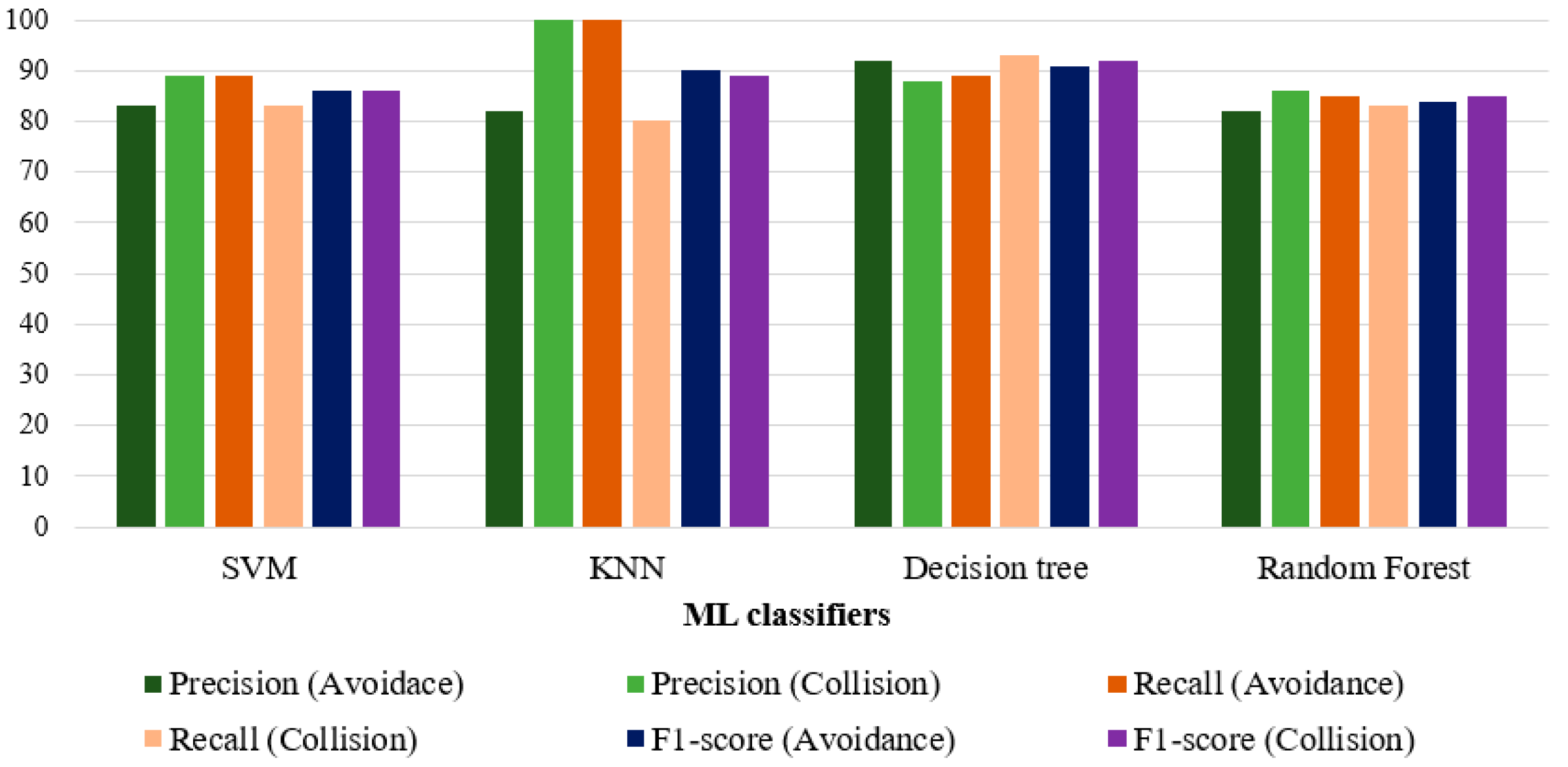
Since the study does not work with linearly separable data, the objective function consists of minimizing the first term, equivalent to maximizing the margin between classes, and a second term, where the error associated with the margin violation is multiplied by a regularization term C. Ideally, the term would be greater than or equal to one, indicating perfect accuracy. However, the introduction of the penalty term C allows controlling the strength of the penalty incurred when a sample is misclassified or within the margin boundary. It is therefore obtained that the highest accuracy values are achieved with a Radial Basis Function (RBF) kernel, Gamma: 1 × 10⁻³, and C = 1000. Note that the value of the regularization parameter C is high enough to state that a lower margin will be accepted if the decision function is better at classifying all the points of the training set correctly. Nevertheless, this high value does not condition the accuracy obtained (86.1%).
(2)
K-nearest neighbors (KNN): It is a classification method that enables us to estimate the density function of the predictors or observations X
i for each class C
j of the response variable or directly the a posteriori probability that this element belongs to the corresponding class. This is a lazy type of learning since the function is approximated only locally, computing from a simple majority vote of the K nearest neighbors of each observation [
41]. This is a robust method when there is noise in the training dataset, especially when the value of K is large in that case. Similarly, if the value of K is high, it can create boundaries between similar classes.
In this model, the distance metric used is Minkowski, so the distances are calculated with the standard Euclidean metric. Applying the GridSearchCV optimization function, the highest accuracy is obtained for K = 8 (91.5%).
On the other hand, the tree-based models considered are:
(3)
Individual decision tree: This is a non-parametric prediction model based on the construction of diagrams with a tree-like structure [
42]. The decision tree divides the sample space into subsets through a series of decision rules by means of a recursive (top-down) partitioning, so that the process ends when the subset at a node has all the same value as the target variable, or when the partition no longer adds value to the predictions.
Different criteria can be used to select the variable and split it successively, although the most usual ones are the Cross-Entropy and Gini index [
43]. Both are based on the probability of each class, adding the logarithmic term in the case of entropy calculation, which makes this criterion computationally more complex. Therefore, and given that both methods yield similar results, the Gini index has been chosen for this study.
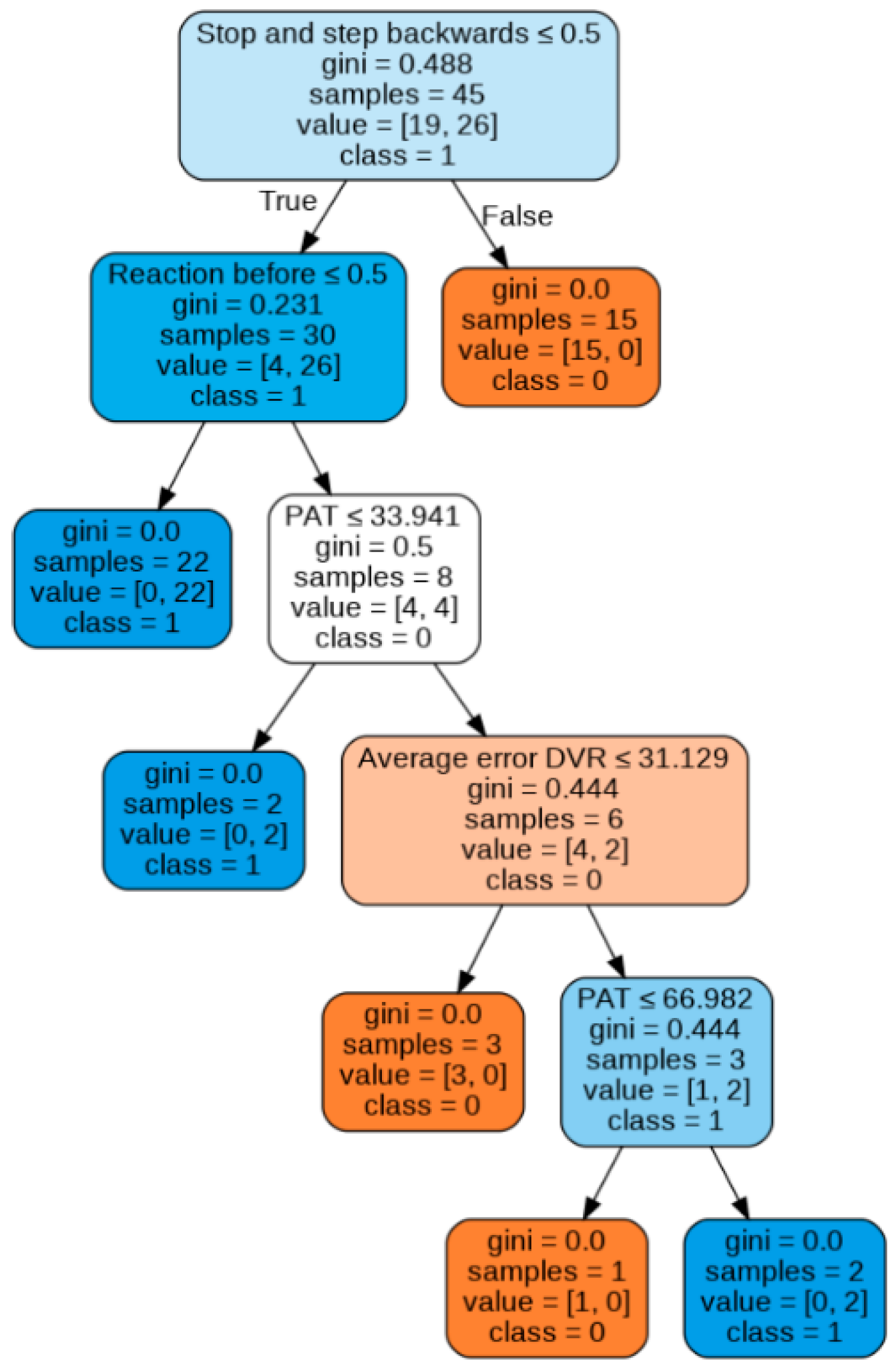
The decision tree was imported from the sklearn.tree module of the Scikit learn Python library. As can be seen in
Figure 13, the first filter on the starting training sample is the type of reaction. In cases where the pedestrian stops and backs up, the accident is avoided. In case of reacting differently (or not reacting at all), any situation that involves not performing such action before the hit lane will imply a collision. In cases where the pedestrian accelerates early before the lane in which the vehicle is traveling, there is a PAT value below 33.9%, since the vehicle starts the simulation implies an accident. If PAT is higher than 33.9%, only in cases with higher visual acuity in the estimation of distances in VR (average error lower than 31.1%), the accident is avoided, while for average error values higher than 31.1%, the accident is avoided with a PAT lower than 67%. The accuracy obtained is 89.85% after k-fold cross-validation is implemented.
(4)
Random Forest: This method [
44] consists of an ensemble of uncorrelated decision trees, the result of which is obtained through the majority vote criterion. The algorithm is based on the bootstrap aggregating or bagging technique, which is based on the random selection of a subsample with a replacement of the training set to feed and fit each of the trees. The advantage of this procedure is better model performance because it reduces the variance of the model, without increasing the bias, and thus reduces sensitivity to the noise that can be obtained with a single tree. In this technique, adding more trees to the model does not increase the risk of over-fitting, but beyond a certain number of trees, no benefit will be achieved. To determine the optimal number of trees, the out-of-bag (OOB) error rate is used as a criterion. The OOB error [
45] is the mean error for each
yi value (calculated using predictions of the trees) that does not contain this observation in its corresponding Bootstrap sample.
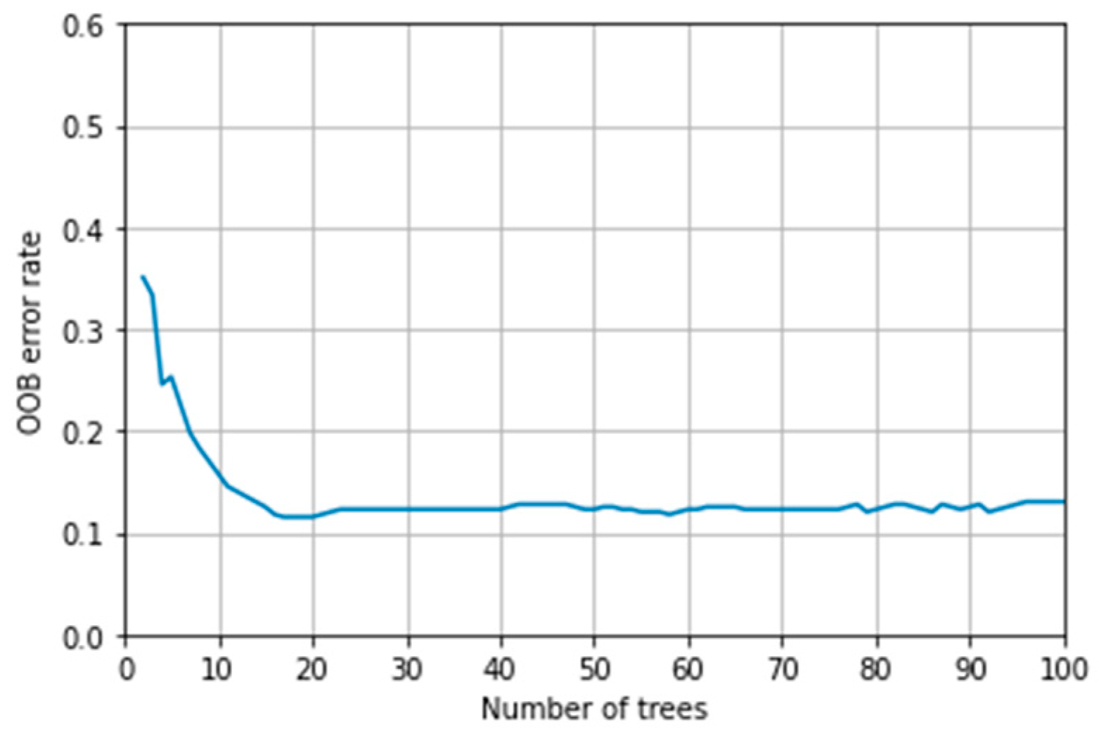
This parameter is calculated by reusing the existing fitted model attributes to initialize the new model in the subsequent call to fit. In this case, this methodology is used to build Random Forest and add more trees, but not to reduce the number of trees. It can be seen in
Figure 14 that, from 24 trees, the OOB error stabilizes and adopts a constant value. Therefore, for a number of trees equal to this value, the Random Forest behaves stably.
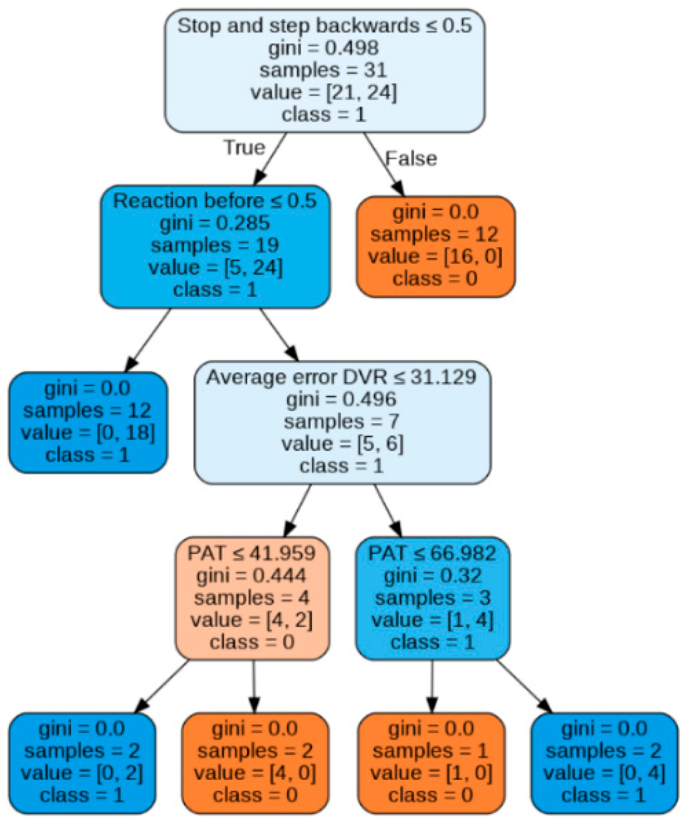
In the example tree shown in
Figure 15, the number of values in the sample does not coincide with the sum of the values of each class. This is due to the implementation of the bootstrapping metalgorithm, which generates new subsets by uniform sampling and replacement over the original dataset, which means that during sample extraction one of the observations can repeatedly come into other samples when fitting the model.
The trees discriminate consistently on the first branches, identifying that reacting once entering the hit-and-run lane ensures collision. As for the individual decision tree, braking is equivalent to avoiding a collision. Complementarily, not reacting or not modifying the walking speed triggers the hit-and-run. For any other reaction (i.e., accelerating) before the run-over lane, a collision is avoided when the average error in the VR distance calculation is lower than 31.1% and the PAT higher than 42%, while for cases where the error is higher than 31%, a collision is avoided only when the PAT is lower than 67%. This method achieves a final accuracy of 84.6%.
The first limitation of both tree models is to assume that in all cases in which the pedestrian stops and backs up, a collision is avoided. However, the error made in this assumption is minimal since this assumption occurs in 96% of the cases (only 1 outlier). The second limitation of these approaches is the lack of logical reasoning in the last node of both models, since avoidance is assured for intermediate values of PAT. However, it hits the target value of two outliers, where an accident occurred even when looking with a sufficiently high PAT, increasing the final accuracy obtained.
The importance of the features [
38] introduced to the model has been determined using two measures: Mean Decrease in Impurity (MDI), and Mean Decrease Accuracy (MDA). The MDI importance metric describes how each individual feature contributes to the decrease in the Gini index across trees, while MDA measurement is defined as the decrease in a model score when a single attribute value is randomly shuffled (permutation). Since the Gini importance measurement may be conditioned by the low cardinality of the features or by those categorical variables with a small number of classes, the evaluation of permutation importance is preferred. For this analysis, a pipeline is built that includes a processing stage for the encoding of the variables and a classifier execution stage, so that the encoding stage can be accessed for the impurity measurement.
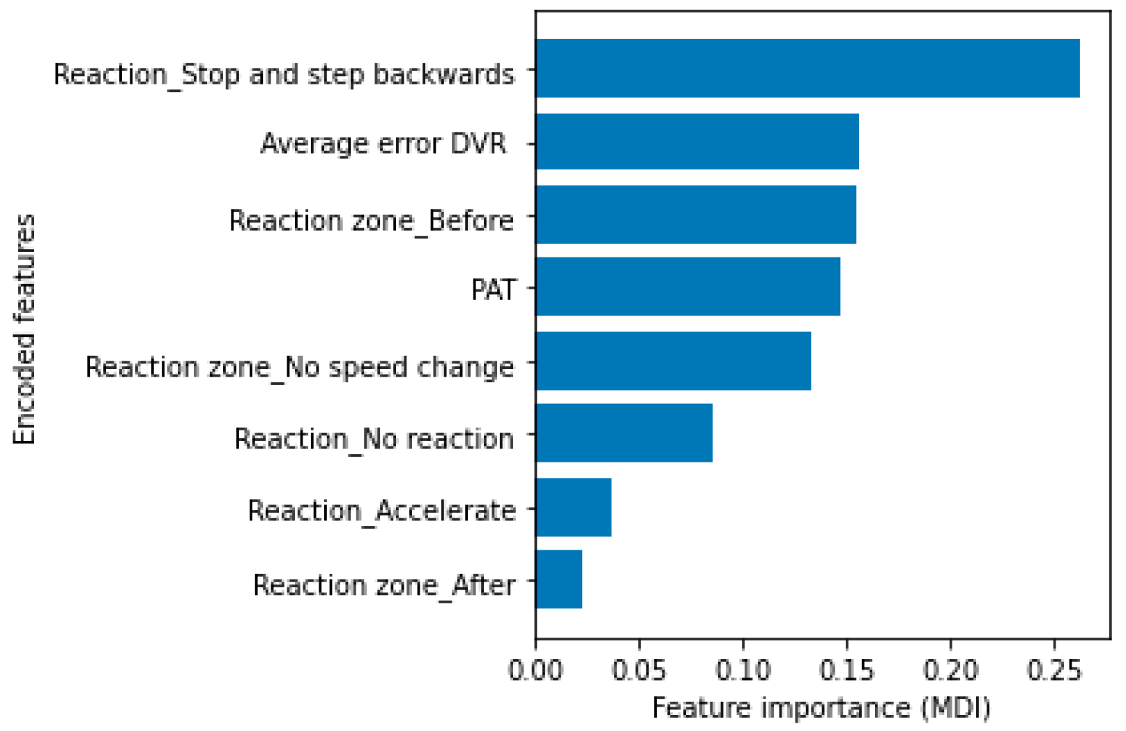
Reaction stopping and backtracking is the most important variable following the MDI metric, followed by reaction before the run-over lane (
Figure 16). In particular, it is possible to see how the impurity-based feature importance inflates the importance of the numerical features “Average error DVR” and “PAT.” This occurs because one of the limitations of the MDI metric is that the calculated importance is biased towards high cardinality features. On the other hand, using the permutation criterion, it is noticeable (
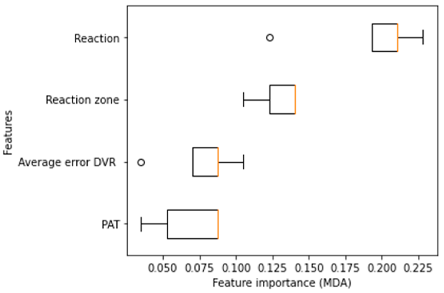
Figure 17) that the reaction type remains the most important feature for the development of the model, followed by the reaction zone, while the numerical variables reach a lower value of importance in the ranking of predictors, as it is reflected in the splitting order of the nodes in both tree models.
Finally,
Table 8 summarizes the optimized parameters that were chosen for each model, corresponding to the previous explanation:


