Abstract
The frequent and sharp fluctuations in garlic prices seriously affect the sustainable development of the garlic industry. Accurate prediction of garlic prices can facilitate correct evaluation and scientific decision making by garlic practitioners, thereby avoiding market risks and promoting the healthy development of the garlic industry. To improve the prediction accuracy of garlic prices, this paper proposes a garlic-price-prediction method based on a combination of long short-term memory (LSTM) and multiple generalized autoregressive conditional heteroskedasticity (GARCH)-family models for the nonstationary and nonlinear characteristics of garlic-price series. Firstly, we obtain volatility characteristic information such as the volatility aggregation of garlic-price series by constructing GARCH-family models. Then, we leverage the LSTM model to learn the complex nonlinear relationships between the garlic-price series and the volatility characteristic information of the series, and predict the garlic price. We applied the proposed model to a real-world garlic dataset. The experimental results show that the prediction performance of the combined LSTM and GARCH-family model containing volatility characteristic information of garlic price is generally better than those of the separate models. The combined LSTM model incorporating GARCH and PGARCH models (LSTM-GP) had the best performance in predicting garlic price in terms of evaluation indexes, such as mean absolute error, root mean-square error, and mean absolute percentage error. The combined model of LSTM-GARCH provides the best results in garlic price prediction and can provide support for garlic price prediction.
1. Introduction
The stability of small-scale agricultural products’ prices is of great significance to the healthy development of the grain market and the national economy. An in-depth understanding of the trends of changes in the prices of small-scale agricultural products plays a guiding role in stabilizing the prices of agricultural products. However, the production of small-scale agricultural products is subject to factors such as planting area and abnormal weather, and their prices often have the characteristics of sharp fluctuations in a short period of time. Take the most representative small-scale agricultural product as an example: the price of Chinese garlic has been extremely unstable in recent years. Affected by a combination of supply and demand, policies, natural disasters, fertilizer prices, oil prices, GDP, public opinion, speculation, and other factors [1], garlic prices in China have experienced many abnormal and precipitous fluctuations. This phenomenon has disrupted normal market expectations [2], affected the interests of industry stakeholders, and even led to market disorder and social unrest [3]. Therefore, with the background of frequent and violent price fluctuations of small-scale agricultural products, it is of great significance to deeply understand the fluctuation trends of small-scale agricultural product prices and explore scientific methods to predict the market prices of them. This could help relevant practitioners make correct judgments and scientific decisions to avoid market risks and promote the healthy development of the small-scale agricultural product industry. This paper takes garlic, the most representative small-scale agricultural product of China, as an example, to explore a price-prediction method for small-scale agricultural products.
The prices of small-scale agricultural products such as garlic are characterized by high volatility, strong nonlinearity, and nonstationarity, and also exhibit some seasonal and cyclical fluctuations [4]. These pose a great challenge to the garlic price prediction task. The prices are influenced by a variety of factors. However, some influencing factors are difficult to measure quantitatively. It is difficult to put all factors in when building a forecasting model. Since these factors are concentrated in the historical price series, it is beneficial to fully explore the volatility characteristics of historical prices to improve the accuracy of the forecasting model. The key to improving prediction performance is to fully exploit the complex regular information in the price series.
Some classical econometric model studies in the past have helped to achieve short-term forecasts of agricultural prices, such as ARIMA, GARCH, and other linear models [5,6,7,8]. However, such models ignore the non-stationary and non-linear characteristics of agricultural price series in modeling and have difficulty capturing the long-term dependence in the series. Moreover, it has been pointed out in the literature that when garlic prices suddenly and dramatically fluctuate, there is still a large gap between the predicted results of the econometric model and the actual values [9].
Machine-learning methods with flexible operational design and powerful self-learning capabilities have been introduced to overcome the shortcomings of econometric models in price forecasting tasks. Such models were found to be effective in learning nonlinear features in time series and improving forecasting performance. They have been shown to be robust in various nonlinear modeling tasks, such as classification and feature extraction [10,11,12]. Among the machine-learning models, artificial neural networks (ANNs) are powerful for predicting nonlinear data [13]. However, due to its shallow structure, the ANN cannot store network states and can hardly deal with the long-term dependence of time series.
Based on this, deep-learning methods have been developed and applied in the field of agricultural product price prediction [14]. Mainstream deep-learning models include the CNN, RNN, and other models [15]. For the time series prediction problem, the recurrent neural network (RNN) is a common and effective method. Still, it often suffers from gradient disappearance or gradient explosion when dealing with long series. Long short-term memory (LSTM) and gated recurrent unit (GRU), which are the variants of the RNN, are starting to emerge. LSTM, proposed by Hochreiter S. [16], and GRU, proposed by Cho [17], address the structural defects of the RNN and can effectively deal with the long short-term dependence and non-linear characteristics of sequences.
In addition, a great deal of research has proved that the linear and nonlinear patterns of price series cannot be captured simultaneously by a single model alone, and agricultural products prices are no exception [18,19,20]. Therefore, combined model methods have been introduced to the agricultural products price prediction task, which combine the advantages of different prediction models by integrating them to capture the linear and nonlinear patterns. Combined models can provide enhanced interpretability while improving the accuracy of price predictions of agricultural products.
Inspired by the above studies, for more accurate prediction of garlic prices, we combined the advantages of deep-learning models and econometric models and propose combined prediction models. The daily garlic-price series is the research object. Since garlic-price series, like those of other financial products, are detected to have heteroskedasticity, we first developed GARCH-family models based on the conditional heteroskedasticity of garlic prices. The GARCH-family models are first used to capture the information of different volatility features, such as volatility aggregation and the leverage effect of garlic-price series. Then, the above volatility feature information is integrated into the bottom layer of the LSTM model, and the self-learning ability of the LSTM model is used to deal with the complex correlations between price information and volatility feature information in the input series to improve the prediction of garlic-price series.
The main contributions of this paper are as follows: (1) This paper proposes a garlic-price-prediction method based on combined model that overcomes the limitations of single-model prediction by incorporating statistical features into deep-learning models. (2) We compared the performances of multiple combined models obtained by merging different GARCH-family models with LSTM, and we present the optimal combined model for garlic price prediction. (3) We compared the LSTM–GARCH combined models with multiple benchmark models and found that LSTM–GARCH combined models are more suitable for the current garlic dataset. It improves on the accuracy of existing garlic price prediction models and provides a new means of garlic price prediction.
The sections of this paper are organized as follows. In Section 2, an overview of related work is introduced. In Section 3, the dataset and details of the prediction models proposed in this paper are described. In Section 4, the experimental procedure and analysis of results of this work are illustrated. Finally in Section 5, the conclusion of the paper is presented.
2. Related Work
Price forecasting is now widely used in various fields; e.g., there are agricultural price forecasting, stock price forecasting, bitcoin volatility forecasting, and oil price forecasting [21,22,23,24,25]. To overcome the limitations of single-model forecasting, forecasting methods have evolved from the initial single models to combined models. This section first reviews the research related to agricultural price forecasting, followed by a review of combined models forecasting research based on econometrics and artificial intelligence in various fields.
2.1. Agricultural Price-Prediction Methods
Common traditional econometric methods include autoregressive integrated moving average (ARIMA) models and generalized autoregressive conditional heteroskedasticity (GARCH) models. The advantages of traditional econometric models lie mainly in the theoretical statistical description of data variables based on logical statistical relationships, which can effectively deal with the linear features in the series and requires a low computational cost for modeling [19]. Wang et al. [5] used the ARIMA model to predict monthly garlic prices, and the experimental results showed that the model was effective for the short-term prediction of garlic prices. Yercan et al. [6] predicted tomato prices in Turkey by using a seasonal ARIMA model and analyzed the seasonal variation in tomato prices. Jadhav et al. [7] validated the effectiveness of the ARIMA model for agricultural product price prediction by using rice and other crop prices. Bhardwaj et al. [8] proposed that GARCH model had an advantage over the ARIMA model for time series data prediction because it captures the volatility agglomeration existing in price data. Ramirez [26] predicted soybean, sorghum, and wheat prices in the U.S. through an asymmetric-error-generalized, autoregressive, conditional heteroskedasticity model. Guo et al. [9] applied the GARCH model to the field of garlic price analysis and prediction and found that the series showed spikes and thick tails, volatility aggregation, and heteroskedasticity. Therefore, garlic price prediction can be achieved by capturing and exploiting the price volatility characteristics. The traditional econometric methods can effectively deal with the linear characteristic relationship of a price series, but its disadvantage is that the prediction performance is not stable in nonlinear sequences.
Machine-learning methods have been used to predict agricultural prices with complex nonlinear relationships [27,28,29]. Jha et al. [13] compared the time delay neural network (TDNN) with the ARIMA model and found that the former enabled better predictions of oilseed price. Li et al. [30] developed a chaotic neural network to predict weekly egg prices in China and found that the chaotic neural network achieved better nonlinear fitting ability and better prediction performance than ARIMA. Hemageetha et al. [31] developed a back propagation neural network (BPNN) to predict tomato prices. Bengio [32] pointed out that shallow neural network structures cannot effectively portray complex nonlinear functions. For this reason, deep learning has been applied to agricultural price prediction. Weng et al. [33] proposed a short-term cucumber price-prediction method based on RNN and found that RNN had better prediction results than BPNN and ARIMA. Jaiswal et al. [14] developed a DLSTM model and found that DLSTM outperformed traditional neural network models and ARIMA model in terms of prediction accuracy and directional changes in price series for nonlinear patterns. Banerjee et al. [34] proposed LSTM to predict vegetable prices and found that LSTM outperformed various benchmark models, including traditional statistical methods and machine-learning methods in both long-term and short-term prediction. Yeong et al. [35] proposed a two-input attention-based LSTM model to predict monthly prices of cabbage and radishes in the Korean market. Since their study applied both feature and temporal attention mechanisms, the feature correlations and temporal relationships among the input variables can be captured, and the prediction performance was improved compared to the benchmark model.
Some scholars have used combination models for agricultural price prediction. Wang et al. [36] predicted the linear and nonlinear components of garlic prices using ARIMA and SVM models, respectively, and finally verified that the combined model outperformed the single ARIMA and SVM models. In addition, other scholars proposed price-prediction methods based on decomposition before integration. Teng et al. [37] used a combined model based on Prophet and SVM to achieve price prediction for ginger. They first used Prophet to decompose the ginger price series. Then, trend and period terms were predicted by Prophet, and the random terms were predicted by SVM. Finally, the ginger price prediction values were recombined by obtained prediction series, and the study showed that the combined model could effectively improve the prediction performance. Xiong et al. [38] proposed the use of extreme learning machine (ELM)-based seasonal trend decomposition (STL) to predict the prices of Chinese cabbage, pepper, cucumber, kidney bean, and tomato, and successfully predicted the prices of vegetables with high seasonality. Liu et al. [18] proposed a prediction method for hog prices based on similar sub-series search and support vector regression. They predicted the cyclical component of the hog price series by using the most similar sub-series search method and predicted the trend component by using support vector regression, and finally recombined the predicted series. They succeeded in addressing the pseudo-cycle problem caused by the varying cycle length. Yin et al. [39] proposed a combined model based on STL, an attention mechanism, and LSTM, and verified the superiority of the combined model by predicting five vegetables: cabbage, radish, onion, pepper, and garlic.
2.2. Combined Models Based on Artificial Intelligence and Econometric Models in General Price Prediction
For general price prediction, combined models based on artificial intelligence and econometric model have been presented [40]. The reason why the models have better prediction performances than the single models is twofold. On the one hand, the econometric models can be dedicated to capturing the linear and volatile characteristics of the price series; on the other hand, the machine learning models can focus on learning the non-linear and nonsmooth characteristics of the price series [24]. Huang et al. [20] proposed to decompose carbon prices into high-frequency and low-frequency sequences using VMD, followed by GARCH to predict high-frequency sequences and LSTM to predict low-frequency sequences, and finally non-linear integration using LSTM; and the results showed that the non-linear integration algorithm could improve the prediction performance of the multi-scale model. Seo et al. [41] proposed to use the output of the GARCH model as the input of the neural network to improve the neural network’s prediction performance. Serkan, Koo, Kakade, and Zolfaghari [21,42,43,44] also proposed to apply a combination of econometric and artificial intelligence models to price forecasting. Table 1 provides the models, forecasting targets, time scales, and conclusions of these studies.

Table 1.
Studies on combined models based on artificial intelligence and econometric models in general price prediction.
For garlic price prediction, we used combined models based on artificial intelligence and an econometric model to improve predictive capabilities. For the heteroskedasticity of garlic-price series, we first built GARCH-family models to extract the fluctuation characteristic information of the price series, and then used the LSTM model to model the non-smoothness and non-linearity in the series in order to improve the performance of garlic price prediction.
3. Materials and Methods
This section gives a detailed explanation of the proposed method. Firstly, a formal description of the data sources of the garlic prediction task used in this research is introduced. Then, the key technologies and algorithms used in the proposed LSTM–GARCH are explained.
3.1. Data Sources
Garlic is grown in a variety of production areas, but the price is mainly determined by a few main production areas. For this reason, the main garlic production area, Jinxiang County in Shandong Province, China, was selected as the study area. In the different links of the cycle of the garlic industry, the wholesale prices of garlic can directly influence the retail prices, and can better reflect the market laws of agricultural product trading compared with the ground price. Therefore, the average daily wholesale price of the Jinxiang market was selected for the experiment. The experimental data source of this paper was the Garlic Industry Chain Big Data Platform developed by the Big Data Center of Shandong Agricultural University. Detailed data were from http://www.garlicbigdata.cn/price/dailyprice.html (accessed on 15 June 2021), and the selected period included a total of 6375 data points from 1 January 2004 to 14 June 2021.
3.2. Symbol Meanings
To facilitate the statement of the content of this paper, we give the notation and descriptions of the symbols used in the proposed method, as shown in Table 2.
Table 2.
List of symbols and descriptions.
3.3. Methods
We propose combined models of LSTM–GARCH-family methods for the garlic price prediction task. To accurately predict garlic price, first we extracted price fluctuation features by using GARCH-family models based on historical price trends of garlic; then we fused historical price information and fluctuation features of garlic, mined garlic price trends, and made price predictions using the LSTM model. In this paper, LSTM–GARCH-family combined models we propose involve the following methods.
3.3.1. LSTM Model
The LSTM model is a special recurrent neural network that solves the gradient disappearance and gradient explosion problems of RNN. It can effectively work out nonlinear variable time series predictions [16]. The core of LSTM is its gating logic. Compared with RNN, LSTM adds an additional neuron called “memory cell” and three gating structures that can control memory cells, input gate, forget gate, and output gate, so LSTM can better handle longer time sequences. The architecture of the model is shown in Figure 1.
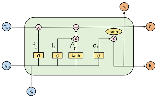
Figure 1.
Internal structure of the LSTM unit.
LSTM processes the garlic price sequence by first determining what kinds of garlic price information are to be retained at the previous moment through a forgetting gate, then determines the garlic price information to be updated and retained in the memory cell through an input gate, and finally determines the predicted garlic price through an output gate. At moment t, there are three inputs to the LSTM. They are , , and , where denotes the garlic price value of the network input at the current moment, denotes the garlic price value of the previous LSTM cell’s output, and denotes the previous LSTM cell state. At moment t, there are two outputs of the LSTM cell. They are and . denotes the output price value of the LSTM cell at the current moment, and is the state of the cell at the current moment. Next, the operation mechanism of LSTM model in garlic price prediction is described in detail.
Forgetting gate. It maps the read and vectors to the (0,1) interval by the sigmoid function and obtains the state calculation of the forgetting gate. indicates the weight of allowing the corresponding information to pass. For example, 0 means the message cannot pass and 1 means that all information can pass. This determines the degree of forgetting of the previous state. The specific formula is
where is the weight matrix of the forgetting gate and is the bias term of the forgetting gate.
Input gate. It first determines the garlic price information to be retained by the sigmoid function. Then, the input content is normalized to the interval (−1,1) by the tanh activation function, generating a new vector and adding it to the cell state. Finally, the old cell state is multiplied bit by bit with an element of the forgetting gate . The new input information is added to update to the new cell state . The specific calculation formula is
where and are the weight matrices of the input gates, and and are the bias terms of the input gates.
Output gate. Determine what to output, which is the predicted price of garlic. The specific formula is
where is the output of the cell state obtained by the sigmoid function and is the garlic price prediction result.
With the above gating structure, LSTM can learn and memorize the effective information of longer time series well and can update and transfer the effective information in the time series. LSTM solves the problem of long-term dependence of RNN. LSTM can extract the sequence features of long time-series data more comprehensively because of storing the long-term interval-effective historical information. The sequences of garlic prices are characterized by high volatility and strong nonlinearity. The LSTM model can better extract the time series characteristics of garlic prices and improve the accuracy of garlic price prediction.
3.3.2. GARCH Family Models
In the analysis and research of time series data, most of the early regression analysis models usually assume that the series variance is constant; i.e., the fluctuation of the time series will not change with time. However, for the prediction problem of the time series of the time-varying volatility, the parameter estimations obtained under the above assumptions are not valid, and the relevant significance tests of the model parameters cannot be performed at this time. GARCH-family models effectively solve these problems and were initially used to analyze financial time series. Its essence is the historical volatility information as a condition and a change in autoregressive form to describe fluctuations. It can better solve the heteroskedasticity, volatility aggregation, leverage effect, and asymmetric effect of the series, so it can better grasp and fit the characteristics of the volatility change of the series.
In 1986, Bollerslev [45] further developed the GARCH model based on the original autoregressive conditional heteroskedasticity model (ARCH). When dealing with garlic-price series, this model is able to describe the effect of a prior period’s external information on the current period’s price fluctuations and the effect of a prior period’s price fluctuations on the sharpness of current price fluctuations through the parameters. The GARCH model can solve the heteroscedasticity and volatility aggregation of garlic-price series. The specific process of the GARCH model is
where is independently and identically distributed and ; is the conditional variance; is the constant; is the ARCH term coefficient; is the GARCH term coefficient; and is the random disturbance term.
As the research progressed, it was found that when the price series is affected by positive and negative shocks the same degree, the impact varies. Generally, most of the positive shocks have less impact on the time series, whereas the negative ones are more powerful and will have a more significant impact on the price series. Such fluctuations are difficult to explain due to the limitations of the GARCH model. Therefore, to further describe this asymmetry, some scholars have started to propose asymmetric GARCH models.
In 1991, Nelson [46] proposed the EGARCH model, which effectively overcomes the drawbacks of the GARCH model. It does not require every coefficient in the variance equation to be nonnegative. By reducing the constraints, the solution process becomes simpler and more flexible. It can describe the leverage effect of the garlic-price series to examine the effect of the nature of information in the market on the degree of volatility. The mean equation of this model is the same as that of the GARCH, and its standard conditional variance equation is
where is the leverage coefficient, and the presence of leverage can be determined by a hypothesis test of . If , it implies that there is asymmetry in the impacts on the shock.
In 1993, Ding Z.X. et al. [47] proposed a PGARCH model for solving asymmetric effects, and the standard conditional variance equation for this model is
where ; when , ; when , , . The power parameter of the standard variance is estimated, rather than specified, to evaluate the magnitude of the impact of the shock on the conditional variance, is the parameter that captures the asymmetric effects up to order r.
Garlic products can be considered as commodities with financial attributes due to storage resistance and easy investment speculation. Based on this, the GARCH-family models are used to analyze the characteristics of garlic price fluctuations and to predict garlic prices. In GARCH modeling, the smoothness test of the price series is performed first. After establishing the mean model, the residuals of the mean model are tested. If there is an ARCH effect, the GARCH model can be established. The specific GARCH-family modeling process is shown in Figure 2.
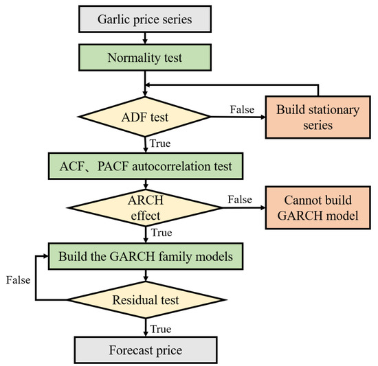
Figure 2.
GARCH-family modeling flowchart.
3.3.3. LSTM and GARCH Family Combined Models
The LSTM model and the GARCH-family models have their advantages in time series data prediction. The LSTM model focuses on capturing the time series features and nonlinear features of the series, whereas the GARCH-family model focuses on analyzing the series from a statistical perspective. To better exploit the garlic-price series’ characteristics and improve the model’s prediction accuracy, this paper explores garlic-price-prediction methods that combine of deep-learning models and econometric models. The specific approach of the combined LSTM–GARCH-family models is as follows.
Different GARCH-family models can capture different information about the economic characteristics of price series. The GARCH, EGARCH, and PGARCH can be used to obtain the characteristics of volatility aggregation and persistence, asymmetric volatility, and enhanced asymmetric volatility flexibility of the series. In the GARCH model, the ARCH term coefficients represent the magnitude of volatility shocks and the GARCH term coefficients represent the persistence of volatility. In the EGARCH model, the leverage coefficient is used to measure the asymmetry of information. When it is positive, it indicates that positive market disturbances cause greater shocks to the volatility of the garlic market than negative disturbances. If it is negative, it indicates that negative market disturbances cause greater shocks to the volatility of the garlic market than positive disturbances. In the PGARCH model, the asymmetric description of serial volatility is represented by the asymmetric effect coefficient. In the combined model, historical prices and the parameters of GARCH-family models, which contain the information of sequence characteristics, are used as the feature inputs of the LSTM model. The combined model can learn more about price fluctuations by introducing statistical features into deep-learning models. Thus, the prediction performance of a combined model can be improved. The LSTM layers in the combined model are used to remember the critical information and forget the unimportant information. When the number of LSTM layers is small, the model has a poor ability to fit the nonlinearity of fluctuating features; when the number of layers is large, the training time is too long and the overfitting phenomenon easily occurs. Based on this, we finally built a stacked LSTM model after several experimental tests, choosing two LSTM layers for fitting the nonlinear features of the sequence and two fully connected layers for data dimensionality reduction, which can take less time to obtain better prediction results on our dataset. Figure 3 shows the structure of an LSTM–GARCH family combined model in this paper.
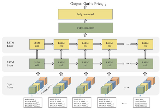
Figure 3.
LSTM–GARCH structure diagram.
Given a current time node, the objective of the LSTM–GARCH family combined model is to predict the garlic price at the current time node based on the historical data for the 50 days prior to that time node. LSTM–GARCH first extracts the volatility feature information from the historical garlic price data using GARCH, EGARCH, and PGARCH. Then, the parameters of GARCH, EGARCH, and PGARCH terms containing volatility feature information for the first 50 days of the time node to be predicted, together with the corresponding price information, are used as the inputs of the LSTM model to train the parameters of the LSTM. Finally, the trained LSTM–GARCH-family model is used for the garlic price prediction task at a certain time node.
4. Experimental Procedure and Analysis of Results
In this section, we present large-scale experiments using the proposed LSTM–GARCH-family combined models and three time-series data-prediction benchmark models on a real dataset. In Section 4.1, we first give the experimental setup to introduce the specific implementation of our experiments. In Section 4.2, we compare and analyze the performances and advantages of LSTM–GARCH and three benchmark models for time series data forecasting in a garlic price forecasting task. In Section 4.3, we present the application of the proposed optimal combined model to the garlic price prediction task.
4.1. Experimental Setup
In the experimental setup, we first introduce the dataset used in our experiments, then give the performance evaluation metrics, and finally describe our experimental design.
4.1.1. Dataset
To improve the generalization ability of the model, the garlic prices from 1 January 2004 to 20 September 2019 were selected as the training data for the model, and the garlic prices from 21 September 2019 to 14 May 2021 were selected as the testing data of the model. In order to reflect the degree of volatility of the garlic-price series and enhance the stability of the series, the first-order difference form of the logarithm of garlic price was constructed, which is =log()-log() (return). We show the time series plot of garlic price return in Figure 4. Subsequently, the ADF unit root test was performed on the series. From Table 3, it is shown that the first-order difference series is smooth. The ARCH Lagrange Multiplier (ARCH-LM) test showed that garlic-price series have a high-order ARCH effect. Therefore, GARCH-family models can be established.
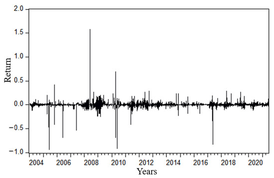
Figure 4.
Average daily price of garlic.
Table 3.
Descriptive statistics and ADF test results.
4.1.2. Evaluation Metrics
The following three evaluation metrics were used to measure the predictive ability of the model: mean absolute error (MAE), root mean-square error (RMSE), and mean absolute percentage error (MAPE). Lower values of the evaluation metrics indicate better performance of the prediction model. The three evaluation metrics were calculated as follows.
where denotes the predicted value of garlic price, denotes the actual price of garlic, and N denotes the total number of predicted samples.
4.1.3. The Structures and Hyperparameters of LSTM–GARCH-Family Combined Models
To illustrate the effectiveness and necessity of the combined models, we first used the GARCH-family models (GARCH, EGARCH, PGARCH) and the LSTM alone for garlic price prediction separately. Second, to find the optimal combined model for garlic price prediction, we combined the LSTM model with the GARCH-family models, and the structures of the combined model are shown in Section 3.3.3. Finally, we compared the performances of the above prediction models to obtain the optimal garlic price prediction model. It summarizes the input layer variables of the single models and the combined models in Table 4. The GARCH terms, EGARCH terms, and PGARCH terms denote the corresponding parameters extracted from the GARCH-family models which were used as inputs to the combined models. In addition, the explanatory variable in Table 4 is the daily price series of garlic, and the symbol “√” denotes input variables in the models.
Table 4.
Input-layer variables of each model.
The choice of parameters is crucial to the prediction performance of the LSTM–GARCH-family combined models. The parameters of the LSTM–GARCH models consisted of two main components. The hyperparameters were used in the LSTM, and the statistical parameters were used to fit the economic model GARCH. To obtain the optimal prediction performances of the models, we iteratively adjusted the parameters of the model. The following was the parameter tuning process for the two types of models used in our experiments.
- Hyperparameter settings in LSTMFor deep-learning models, prediction performance is highly dependent on the choice of hyperparameters. Since the hyperparameter space is large and cannot be fully traversed, we used empirical tuning to get the hyperparameters with good performances for the selected dataset. The essential hyperparameters, such as learning rate, batch size, sliding window size, and the number of LSTM neurons, significantly influenced the model’s performance when building the model. For the hyperparameters selected for LSTM, we used MSE as the loss function. In addition, Adam was used as an optimizer, which combines the advantages of AdaGrad and RMSProp, including fast convergence and small memory requirements [48].For the learning rate setting, due to the learning rate being set to 0.001, the model converged faster and the accuracy was higher. We set the learning rate to 0.001. The computational time of the model was about 219.4s.For the values of batches and windows hyperparameters, we set the initial batches to and windows to . Next, we performed combined optimization of batches and windows. Figure 5 shows the results of the corresponding hyperparameter configurations; the final values of batches and windows were set to 40 and 50. In addition, we use Figure 6a to show the performance of LSTM with varying window values when the initial batch value is 40. We use Figure 6b to show the performance of LSTM with varying batch values when the initial window’s value is 50.
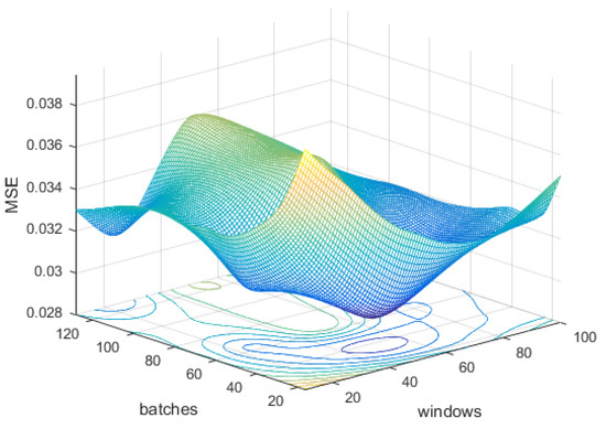 Figure 5. 3D fitting diagram of LSTM’s performance with different numbers of batches and windows.
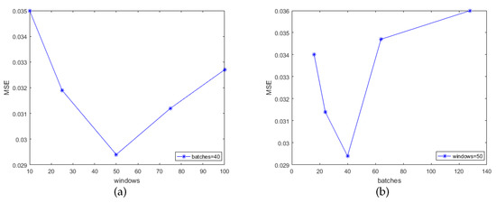 Figure 6. Performance comparison of LSTM with different numbers of batches and windows. (a) The performance of LSTM with varying numbers of windows when batches number is 40. (b) The performance of LSTM with varying batch size when windows number is 50.To select the number of neurons, we first chose from and then fine-tuned them in the appropriate interval to achieve the ideal state. Finally, 20 neurons were selected for the first LSTM layer and ten neurons for the second LSTM layer.
- Parameter settings in GARCHFor econometric models, we chose to use the GARCH, EGARCH, and PGARCH from the GARCH-family models. The error distributions were the Student’s t distribution and the GED distribution. In GARCH, , , and . The results of the GARCH model with different parameters are shown in Table 5. According to the AIC, SC, and HQ criteria (the smaller the value, the better the model fit), the optimal GARCH model was selected among multiple GARCH models. The rules for EGARCH and PGARCH model selection were the same. We finally chose the GARCH, EGARCH, and PGARCH models by the GED distribution.
Table 5. AIC, SC, and HQ results of the GARCH model with different parameters.
The LSTM prediction model consisted of three basic modules: the input layer, the hidden layer, and the output layer. The key hyperparameters were set as shown in the hyperparameter settings section. In the LSTM model, the numbers of neurons in the two LSTM layers were 20 or 10, and the numbers of hidden nodes in the two fully connected layers were 5 and 1, respectively. A small batch of data with 40 points was selected for iterative training in this experiment. To avoid overfitting the data, dropout regularization was used, and the probability was set to 0.1 [49]. The garlic price of the last 50 days was selected to predict the garlic price of the next day. Meanwhile, Adam was chosen and a learning rate of 0.001 was set to control the learning speed of the network. After 100 epochs, the model loss stopped decreasing and reached a state of convergence.
GARCH-family single model prediction. In the part of parameter-setting discussion, we introduced how to choose the parameters of the GARCH-family models. Based on AIC, SC, and HQ criteria, we chose the GARCH (1, 1, 0), EGARCH (1, 1, 1), and PGARCH (1, 1, 1) models under the GED distribution. We could predict the garlic price through the established models. Meanwhile, the characteristic term coefficients of the GARCH-family models were derived.
Single-combination model prediction. GARCH-family models were combined with an LSTM model to obtain LSTM–GARCH (LSTM-G), LSTM-EGARCH (LSTM-E), and LSTM-PGARCH (LSTM-P). The hyperparameters were the same as in the LSTM model, except that the number of LSTM-layer neurons changed slightly with the input dimensions. We tested the accuracy of different numbers of hidden nodes through many experiments to obtain the prediction results with the highest accuracy. According to the rules for selecting LSTM layer neurons already introduced in the discussion of parameter settings, we set the numbers of neurons in the two LSTM layers of the single combined models to 25 and 10, and the numbers of nodes in the fully connected layers to 5 and 1. Similarly, single-combination models reach eda state of convergence after 100 epochs.
Dual-model prediction. The two GARCH-family models were combined with the LSTM model to obtain the dual-combination models LSTM-GE, LSTM-GP, and LSTM-EP. We adjusted hyperparameters such as the number of neurons in the LSTM layer of the model to construct a well-performing garlic prediction model. The final numbers of neurons in the LSTM layers were chosen to be 30 and 10, respectively; and the numbers of nodes in the fully connected layers were 5 and 1, respectively.
Triple-combination model prediction. The three GARCH-family models were combined with the LSTM model to obtain the triple combination model LSTM-GEP. The final numbers of neurons in the LSTM layers were chosen to be 30 and 15, respectively; and the numbers of nodes in the fully connected layer were 5 and 1, respectively.
4.1.4. Benchmark Models
To further demonstrate the effectiveness and superiority of our proposed model, we selected three prediction models and compared them with our proposed model. First, we selected CNN and GRU models and combined them with GARCH-family models to obtain GRU–GARCH-family models and CNN–GARCH-family models as benchmark models. In addition, we also selected the attention–LSTM model, which has an excellent performance in current time series data prediction, to compare with our proposed optimal LSTM–GARCH family model.
- GRU has a similar structure to the LSTM and can be regarded as a simple variant of LSTM. Both LSTM and GRU preserve important features through various gate structures and thus ensure they will not be lost even after a long period. GRU improves the complex cell structure of LSTM by merging the input and forgetting gates and merging the cell states and hidden states of LSTM. In the GRU model, the reset gate is used to determine how much past information to forget, and the update gate is used to decide how much input and previous output to pass to the next cell, so the GRU cell can decide how much information to copy from the past to reduce the risk of gradient disappearance. It has often been applied to price prediction in recent years [50]. The performances of LSTM and GRU are slightly different on different data sets. To further verify the superiority of our proposed model, we combined the GRU with the GARCH-family models to obtain the GRU–GARCH-family combined models. The GRU and GRU–GARCH-family models were selected as the benchmark models. We built a stacked GRU model similar to the LSTM model, i.e., with two GRU layers and two fully connected layers. With the hyperparameters adjusted to the optimal case, the optimal LSTM–GARCH-family combined models we obtained in the above experiments were compared with the GRU and GRU–GARCH-family combined models (GRU-G, GRU-GP, and GRU-GEP).
- A convolutional neural network (CNN) is suitable for spatial feature extraction and is widely used in the field of image recognition. It mainly includes an input layer, a convolutional layer, a pooling layer, a fully connected layer, and an output layer. We tried to use the CNN model for garlic price prediction work. In this work, the CNN model took garlic price and GARCH-family-related parameters as input data and extracted the correlation between each index and garlic price through convolution operation; then compressed the amount of data and parameters through pooling to avoid overfitting and reduce the complexity of the model; then transformed the data form through flattening layer; and finally fine-tunesd and output the prediction results using a fully connected layer. We combined the CNN with the GARCH-family models to get CNN–GARCH-family combined models to test the ability of the CNN to extract garlic-price series features. We compared the optimal LSTM–GARCH-family models with the combined CNN–GARCH-family models (CNN-G, CNN-GP, and CNN-GEP). We set the CNN to have two convolutional layers, a max pooling layer, a dropout layer, and a fully connected layer ui a grid search method. For the first two convolutional layers, the filter size was 1 and the numbers of filters were selected as 32 and 16, respectively. The filter size for the max pooling layer was 2. In addition, dropout regularization was set to 0.1 to prevent overfitting.
- Attention improves the model’s ability to select temporal correlations. The attention mechanism is a resource allocation mechanism that mimics human attention, and it can change the level of attention to input information by assigning reasonable weights to different features. Attention–LSTM models are often used in the field of price prediction. Many extant pieces of literature point out that LSTM incorporating the attention mechanism has an advantage over LSTM models in time-series data prediction. Therefore, we selected an attention–LSTM as a benchmark model. For a fair comparison, the attention–LSTM model had two LSTM layers, and the hyperparameters of the LSTM layers were the same as those of the solo LSTM. In addition, we added the attention layer after the two LSTM layers.
4.2. Analysis of Results
In the analysis of results, we first analyze the performance of our proposed LSTM–GARCH-family combined models and then compare the optimal combined model with the benchmark models. In this paper, we use the three evaluation metrics, MAE, RMSE, and MAPE, to evaluate the performances of the garlic price prediction models; smaller values indicate better prediction performance.
4.2.1. Results of LSTM–GARCH-Family Models
The results of the LSTM–GARCH family combined models are shown in Table 6. From the experimental results, it can be seen that the prediction performance of the LSTM model is significantly better than those of the GARCH-family models alone. The values of MAE, RMSE, and MAPE for the LSTM model were 12.87%, 16.73%, and 5.21%, which are significantly lower than those of the GARCH, EGARCH, and PGARCH models. Compared with the GARCH-family models, the LSTM model can learn the temporal patterns and nonlinear characteristics of time series data more effectively due to its long memory. Figure 7a shows the prediction results of the LSTM model in the test set.
Table 6.
Performance comparison among different models.
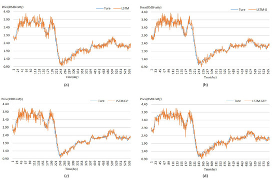
Figure 7.
The prediction results of the models on the test set. (a) LSTM, (b) LSTM-G, (c) LSTM-GP, (d) LSTM-GEP.
In the combined models, the prediction performance was significantly improved over the LSTM model. Due to the addition of a GARCH-family model, the single combined models captured the information of economic characteristics in the garlic-price series. The experimental results show that LSTM-G had the best prediction performance among the single combined models. By adding GARCH coefficients to the input layer of LSTM, the LSTM-G model captured the information of economic characteristics, such as volatility aggregation and volatility persistence of garlic-price series. Thus, the model prediction performance was significantly improved; and its values of MAE, RMSE, and MAPE were reduced to 11.88%, 16.00%, and 4.87%. Similarly, LSTM-E and LSTM-P, by the addition EGARCH coefficients and PGARCH coefficients to the input layer of LSTM, respectively, enable the models to capture the leverage effect of garlic-price series and enhance the flexibility of asymmetric fluctuations of the time series. GARCH coefficients had the highest contribution to the improvement of model performance among the single combined models. Figure 7b shows the prediction results of the LSTM-G combination model in the test set.
Compared to the single models and single-combination models, it was found that the dual-combination models have better prediction performances. The LSTM-GP combined model had the best prediction performance. The combination of GARCH coefficients and PGARCH coefficients had the highest contribution to the improvement of model performance in the dual-combination models. The LSTM-GP model had the smallest MAE, RMSE and MAPE values of 11.44%, 15.66%, and 4.56%, respectively. Figure 7c shows the prediction results of the LSTM-GP model in the test set.
The prediction performance of the LSTM-GEP combined model merged with three GARCH-family models did not further improve on the dual-combination models. Further additions did not provvide better prediction performance. Figure 7d shows the prediction results of the LSTM-GEP combination model in the test set.
From the overall prediction results, it can be seen that the deep-learning model outperformed the econometric models and the combined models generally performed better than the single models. The combined models use the GARCH-family models to capture the fluctuation characteristic information of the garlic-price series, which effectively expands the price series information, thereby enabling the LSTM model to learn more effective information. Therefore, the prediction performances of combined models were effectively improved. Figure 8 shows the percentage reductions of MAE, RMSE, and MAPE of the better performing combined models compared with the LSTM model, and it was found that the LSTM-GP combined model had the most significant reduction of evaluation metrics, indicating that the LSTM-GP combined model has the best prediction performance.
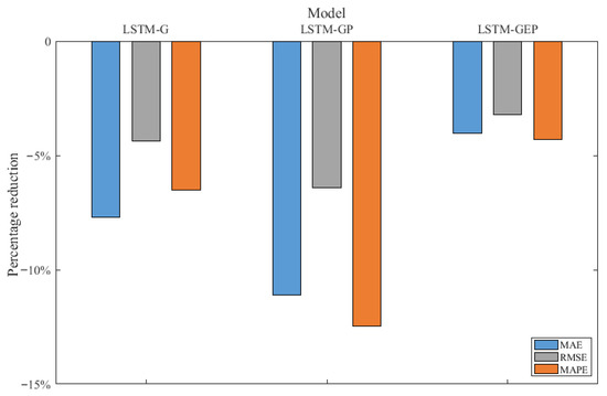
Figure 8.
Comparison of MAE, RMSE, and MAPE between the combined models and LSTM model.
4.2.2. Results of Comparison with the Benchmark Models
The results of the prediction performance comparison between the proposed optimal combined model LSTM-GP and the three sets of benchmark models are shown in Figure 9a–c. It can be seen from the figures that the prediction performance of LSTM-GP was better than that of the GRU–GARCH combined models, the CNN–GARCH-family combined models, and the LSTM model with an attention mechanism. Below we analyze the reasons in detail.
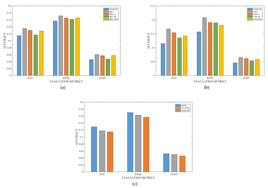
Figure 9.
Comparison of MAE, RMSE, and MAPE among the proposed optimal model, the GRU–GARCH models, the CNN–GARCH combined models, and the attention–LSTM model. (a) Comparison between the proposed optimal model and the GRU–GARCH family combined models. (b) Comparison between the proposed optimal model and the CNN–GARCH family combined models. (c) Comparison among the proposed optimal model, attention–LSTM model, and LSTM model.
First, we compare and analyze the performances of the models obtained by combining LSTM, GRU, and CNN with GARCH-family models. From Figure 9a,b, we found that all three types of deep-learning models combined with GARCH-family models improved the prediction performances more than single deep-learning models. The results of the three types of combined models, LSTM–GARCH, GRU-GARCH, and CNN-GARCH, proved that combining deep-learning models with GARCH-family models can improve the prediction performance. The reason is that the GARCH-family models expand the historical price information by calculating the price volatility at each time node and mining the price volatility features at each time node, which enables the deep-learning models to capture feature information other than price and effectively improve the prediction performances of the models. Among them, the addition of GARCH and PGARCH models contributed the most to improving performance.
Second, we compare and analyze the extraction abilities of three deep-learning models, LSTM, GRU, and CNN, for garlic price sequence features. From Figure 9a,b, it can be seen that among the various types of single and combined models, the LSTM-GP model produced the lowest MAE, RMSE, and MAPE metrics, which proves that LSTM has the best extraction ability for garlic-price series features. We briefly analyzed the reasons in terms of the three types of model structures. Although the CNN can capture the spatial structure of data, it does not have a long-term memory function and lacks consideration of the correlation of time-series data. Hence, its prediction performance is inferior to those of LSTM and GRU. Compared with the LSTM model, although the GRU improves computational efficiency by simplifying the gate structure, GRU has a slightly inferior performance to LSTM. The LSTM-GP model has the best performance and outperformed the GRU-GP and CNN-GP models.
Finally, to verify the effectiveness of the LSTM-GP model, we compared it with the attention–LSTM model, which shows a better current temporal prediction effect. Figure 9c shows that the LSTM model with the attention mechanism has better prediction performance than the LSTM model alone. The reason is that by adding the attention mechanism, the LSTM model can take into account the importance of different hidden states and focus more attention on the relatively essential states. Therefore, the model can better capture the sequence’s long-term dependencies. Compared to the LSTM model with the attention mechanism, the LSTM-GP model, by simultaneously capturing characteristic information such as volatility aggregation and temporal correlation of garlic-price series, captures more effective information at each time node. For this reason, our proposed combined LSTM-GP model produced lower values for the three evaluation metrics and better performance in garlic price prediction.
4.3. Price Prediction Analysis
According to the above research on garlic-price-prediction methods, the combined LSTM-GP model has the highest prediction accuracy. To further verify the effectiveness of the model, we predicted garlic prices for a total of 31 days from 15 May 2021 to 14 June 2021, by using LSTM-GP, and analyzed the prediction performance. A comparison of the predicted results with the actual prices is shown in Figure 10; and MAE, RMSE, and MAPE of the models are shown in Figure 11. MAE, RMSE, and MAPE were 0.1143, 0.1400, and 4.40%, which are 16.93%, 17.93%, and 17.47% lower than those of the LSTM model. From Figure 10, we can see that the predicted values of the combined LSTM-GP model are closer to the actual prices than those of LSTM. This also confirms that the price series features extracted by the GARCH-family models help to improve the prediction performance of the model. Through empirical analysis, it can be concluded that the model is effectively and stably applicable to the short-term prediction of garlic prices and has a certain degree of interpretability to support the prediction of garlic prices.
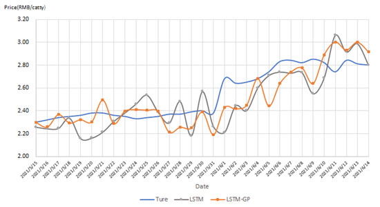
Figure 10.
Comparison of prices predicted by the LSTM-GP model and real prices.
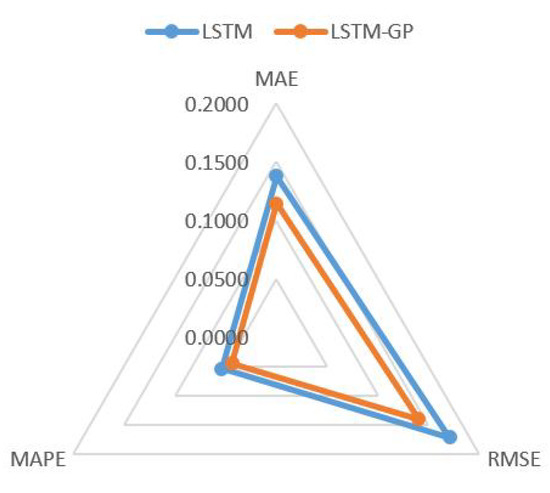
Figure 11.
Comparison of MAE, RMSE, and MAPE between LSTM-GP and LSTM.
5. Conclusions
Aiming at the characteristics of high volatility, strong nonlinearity, and nonsmoothness of garlic daily price series, this paper proposed a method combining a deep-learning model and econometric model to construct a garlic price prediction model based on a GARCH-family model and an LSTM model. The volatility characteristics of garlic-price series were extracted by the GARCH-family models, and then the parameters obtained from the GARCH-family models containing volatility characteristics information and price series were added to the LSTM model input layers. The volatility characteristics of the garlic-price series were fully learned by using the self-learning ability and long-time memory of the LSTM model. It has the respective advantages of the two types of models, thereby improving the model’s prediction performance. Large-scale experiments based on real data led to the following conclusions.
(1) Among the single models, the LSTM model performs significantly better than the GARCH-family models. By using its long memory property to effectively learn the temporal patterns of time series, LSTM can deal with the complex nonlinear relationships in garlic-price series and overcome the shortcoming of low accuracy in traditional prediction models.
(2) The prediction performances of the combined models were generally better than those of the single model. The combined models of the LSTM and GARCH family introduce the statistical features of garlic price data into the deep-learning model and reasonably exploit the linear and nonlinear information in the price data. The combined models outperformed the single models in the evaluation indexes of mean absolute error, root mean-square error, and mean absolute percentage error.
(3) The LSTM-GP combined model, which incorporates GARCH, PGARCH, and LSTM models, had the best performance of all models. The empirical analysis concluded that the model is effectively applicable to the short-term prediction of garlic prices and has a certain degree of interpretability, which can provide support for garlic price prediction.
In light of the results obtained, we have proposed a combined model that is applicable to garlic price prediction called LSTM–GARCH. The model proposed in this paper, which was studied from a time series perspective, solves the problems of low prediction accuracy of the traditional single model and poor model interpretability of existing price prediction models. It can effectively achieve the short-term prediction of garlic prices. The accurate prediction of garlic prices can help people related to the garlic industry chain to make correct judgments and scientific decisions, which is conducive to avoiding market risks and can play a guiding role in stabilizing the market for this small agricultural commodity.
Currently, the combined model we have constructed has not been put into use. Alfonso et al. [51] proposed a broad set of intelligent agents that achieve cryptocurrency prediction and can be used for actual trading. Inspired by this, we are considering further completing the garlic price prediction system in the garlic industry chain big data platform we developed. Second, it is worth considering that garlic, as an important small agricultural product, is subject to multiple uncertainties, such as supply and demand, speculative behavior, and public opinion. This poses a specific challenge to garlic price prediction. In the future, we may adopt multi-view learning to integrate garlic-price-influencing factors based on garlic prices and explore the construction of a multi-feature combined model to improve garlic price prediction accuracy further.
Author Contributions
Conceptualization, methodology, and writing—original draft preparation, Y.W. and P.L.; software, Y.W.; writing—review and editing, validation, K.Z. and L.L.; formal analysis investigation, supervision, and project administration, Y.Z.; resources, visualization, and data curation, G.X. All authors have read and agreed to the published version of the manuscript.
Funding
This research was funded by the Major Agricultural Applied Technology Innovation Project of Shandong Province, grant number SD2019ZZ019; the Key Research Development Program (Major Science and Technology Innovation Projects) of Shandong Province, grant number 2022CXGC010609; and the Major Science and Technology Innovation Project of Shandong Province, grant number 2019JZZY010713.
Institutional Review Board Statement
Not applicable.
Informed Consent Statement
Not applicable.
Data Availability Statement
Not applicable.
Acknowledgments
Thanks to the Key Laboratory of Huang-Huai-Hai Smart Agricultural Technology, Ministry of Agriculture and Rural Affairs, for its support for scientific research.
Conflicts of Interest
The authors declared no conflict of interest.
References
- Zhang, X.X.; Liu, L.; Su, C.W.; Tao, R.; Lobon, O.R.; Moldovan, N.C. Bubbles in agricultural commodity markets of China. Complexity 2019, 2019, 2896479. [Google Scholar] [CrossRef]
- Chen, W.J.; Guo, F.; Zhang, C.; Liu, P.Z.; Ren, W.M.; Cao, N.; Ding, J.R. Development and application of big data platform for garlic industry chain. Comput. Mater. Contin. 2019, 58, 229–248. [Google Scholar] [CrossRef]
- Wu, G.J.; Zhang, C.; Liu, P.Z.; Ren, W.M.; Zheng, Y.; Guo, F.; Chen, X.W.; Russell, H. Spatial quantitative analysis of garlic price data based on arcgis technology. Comput. Mater. Contin. 2019, 58, 183–195. [Google Scholar] [CrossRef]
- Guo, F.; Liu, P.Z.; Ren, W.M.; Cao, N.; Zhang, C.; Wen, F.J.; Zhou, H.M. Research on the relationship between garlic and young garlic shoot based on big data. Comput. Mater. Contin. 2019, 58, 363–378. [Google Scholar] [CrossRef]
- Wang, B.; Liu, P.; Zhang, C.; Wang, J.; Liu, P. Prediction of garlic price based on arima model. In Proceedings of the 4th International Conference on Cloud Computing and Security (ICCCS), Haikou, China, 8–10 June 2018; pp. 731–739. [Google Scholar] [CrossRef]
- Adanacioglu, H.; Yercan, M. An analysis of tomato prices at wholesale level in turkey: An application of sarima model. Custos E Agronegocio 2012, 8, 52–75. [Google Scholar]
- Jadhav, V.; Reddy, B.V.C.; Gaddi, G.M. Application of arima model for forecasting agricultural prices. J. Agric. Sci. Technol. 2017, 19, 981–992. [Google Scholar]
- Bhardwaj, S.; Paul, R.K.; Singh, D.; Singh, K. An empirical investigation of arima and garch models in agricultural price forecasting. Econ. Aff. 2014, 59, 415. [Google Scholar] [CrossRef]
- Guo, F.; Liu, P.Z.; Ren, W.M.; Cao, N.; Zhang, C.; Wen, F.J.; Zhou, H.M. Research on the law of garlic price based on big data. Comput. Mater. Contin. 2019, 58, 795–808. [Google Scholar] [CrossRef]
- Jang, B.; Kim, M.; Harerimana, G.; Kang, S.U.; Kim, J.W. Bi-lstm model to increase accuracy in text classification: Combining word2vec cnn and attention mechanism. Appl. Sci. 2020, 10, 5841. [Google Scholar] [CrossRef]
- Alfonso, G.; Nicola, L.; Delfina, M.; Rocco, Z.; Carmine, C. Automatic users’ gender classification via gestures analysis on touch devices. Neural Comput. Appl. 2022, 34, 18473–18495. [Google Scholar] [CrossRef]
- Li, Y.F.; Ngom, A. Data integration in machine learning. In Proceedings of the 2015 IEEE International Conference on Bioinformatics and Biomedicine (BIBM), Washington, DC, USA, 9–12 November 2015; pp. 1665–1671. [Google Scholar] [CrossRef]
- Jha, G.K.; Sinha, K. Time-delay neural networks for time series prediction: An application to the monthly wholesale price of oilseeds in india. Neural Comput. Appl. 2014, 24, 563–571. [Google Scholar] [CrossRef]
- Jaiswal, R.; Jha, G.K.; Kumar, R.R.; Choudhary, K. Deep long short-term memory based model for agricultural price forecasting. Neural Comput. Appl. 2021, 34, 4661–4676. [Google Scholar] [CrossRef]
- Yang, Y.R.; Xiong, Q.Y.; Wu, C.; Zou, Q.H.; Yang, Y.; Yi, H.L.; Gao, M. A study on water quality prediction by a hybrid CNN-LSTM model with attention mechanism. Environ. Sci. Pollut. Res. 2021, 28, 55129–55139. [Google Scholar] [CrossRef] [PubMed]
- Hochreiter, S.; Schmidhuber, J. Long short-term memory. Neural Comput. 1997, 9, 1735–1780. [Google Scholar] [CrossRef] [PubMed]
- Cho, K.; Van Merrienboer, B.; Gulcehre, C.; Bahdanau, D.; Bougares, F.; Schwenk, H.; Bengio, Y. Learning Phrase Representations using RNN Encoder-Decoder for Statistical Machine Translation. arXiv 2014, arXiv:1406.1078. [Google Scholar]
- Liu, Y.; Duan, Q.; Wang, D.; Zhang, Z.; Liu, C. Prediction for hog prices based on similar sub-series search and support vector regression. Comput. Electron. Agric. 2019, 157, 581–588. [Google Scholar] [CrossRef]
- Kim, H.Y.; Won, C.H. Forecasting the volatility of stock price index: A hybrid model integrating lstm with multiple garch-type models. Expert Syst. Appl. 2018, 103, 25–37. [Google Scholar] [CrossRef]
- Huang, Y.; Dai, X.; Wang, Q.; Zhou, D. A hybrid model for carbon price forecasting using garch and long short-term memory network. Appl. Energy 2021, 285, 116485. [Google Scholar] [CrossRef]
- Serkan, A. Stacking hybrid GARCH models for forecasting Bitcoin volatility. Expert Syst. Appl. 2021, 174, 114747. [Google Scholar] [CrossRef]
- Ye, K.; Piao, Y.; Zhao, K.; Cui, X. A heterogeneous graph enhanced lstm network for hog price prediction using online discussion. Agriculture 2021, 11, 359. [Google Scholar] [CrossRef]
- Jin, Z.G.; Yang, Y.; Liu, Y.H. Stock closing price prediction based on sentiment analysis and lstm. Neural Comput. Appl. 2020, 32, 9713–9729. [Google Scholar] [CrossRef]
- Liu, J.W.; Huang, X.H. Forecasting crude oil price using event extraction. IEEE Access 2021, 9, 149067–149076. [Google Scholar] [CrossRef]
- Busari, G.A.; Lim, D.H. Crude oil price prediction: A comparison between AdaBoost-LSTM and AdaBoost-GRU for improving forecasting performance. Comput. Chem. Eng. 2021, 155, 107513. [Google Scholar] [CrossRef]
- Ramirez, O.A.; Fadiga, M.L. Forecasting agricultural commodity prices with asymmetric-error garch models. West. J. Agric. Econ. 2003, 28, 71–85. [Google Scholar] [CrossRef]
- Yang, L.; Li, K.; Zhang, W.; Kong, Y. Short-term vegetable prices forecast based on improved gene expression programming. Int. J. High Perform. Comput. Netw. 2018, 11, 199–213. [Google Scholar] [CrossRef]
- Zhang, Y.; Na, S. A novel agricultural commodity price forecasting model based on fuzzy information granulation and mea-svm model. Math. Probl. Eng. 2018, 2018, 2540681. [Google Scholar] [CrossRef]
- Liu, Y.; Gong, C.; Yang, L.; Chen, Y. Dstp-rnn: A dual-stage two-phase attention-based recurrent neural network for long-term and multivariate time series prediction. Expert Syst. Appl. 2020, 143, 113082. [Google Scholar] [CrossRef]
- Li, Z.M.; Cui, L.G.; Xu, S.W.; Weng, L.Y.; Dong, X.X.; Li, G.Q.; Yu, H.P. Prediction model of weekly retail price for eggs based on chaotic neural network. J. Integr. Agric. 2013, 12, 2292–2299. [Google Scholar] [CrossRef]
- Hemageetha, N.; Nasira, G.M. Radial basis function model for vegetable price prediction. In Proceedings of the International Conference on Pattern Recognition, Salem, India, 21–22 February 2013. [Google Scholar] [CrossRef]
- Bengio, Y. Learning Deep Architectures for AI; Now Publishers Inc.: Boston, MA, USA, 2009. [Google Scholar]
- Weng, Y.; Wang, X.; Hua, J.; Wang, H.; Kang, M.; Wang, F. Forecasting horticultural products price using arima model and neural network based on a large-scale data set collected by web crawler. IEEE Trans. Comput. Soc. Syst. 2019, 6, 547–553. [Google Scholar] [CrossRef]
- Banerjee, T.; Sinha, S.; Choudhury, P. Long term and short term forecasting of horticultural produce based on the lstm network model. Appl. Intell. 2022, 52, 9117–91147. [Google Scholar] [CrossRef]
- Yeong, H.G.; Dong, J.; Helin, Y.; Ri, Z.; Xianghua, P.; Seong, J.Y. Forecasting agricultural commodity prices using dual input attention lstm. Agriculture 2022, 12, 256. Available online: https://www.mdpi.com/2077-0472/12/2/256 (accessed on 1 October 2022).
- Wang, B.; Liu, P.; Zhang, C.; Wang, J.; Chen, W.; Cao, N.; Wen, F. Research on hybrid model of garlic short-term price forecasting based on big data. Comput. Mater. Contin. 2018, 57, 283–296. [Google Scholar] [CrossRef]
- Teng, J.; Wang, X.; Zhang, Y.; Wen, F.; L, P. Research on ginger price prediction based on prophet- support vector machine (svm) combination model. Direct Res. J. Agric. Food Sci. 2020, 8, 340–345. [Google Scholar]
- Xiong, T.; Li, C.; Bao, Y. Seasonal forecasting of agricultural commodity price using a hybrid stl and elm method: Evidence from the vegetable market in china. Neurocomputing 2018, 275, 2831–2844. [Google Scholar] [CrossRef]
- Yin, H.; Jin, D.; Gu, Y.H.; Park, C.J.; Han, S.K.; Yoo, S.J. Stl-attlstm: Vegetable price forecasting using stl and attention mechanism-based lstm. Agriculture 2020, 10, 612. [Google Scholar] [CrossRef]
- Hu, Y.; Ni, J.; Wen, L. A hybrid deep learning approach by integrating LSTM-ANN networks with GARCH model for copper price volatility prediction. Phys. A Stat. Mech. Its Appl. 2020, 557, 124907. [Google Scholar] [CrossRef]
- Seo, M.; Kim, G. Hybrid forecasting models based on the neural networks for the volatility of bitcoin. Appl. Sci. 2020, 14, 4768. [Google Scholar] [CrossRef]
- Koo, E.; Kim, G. A Hybrid Prediction Model Integrating GARCH Models with a Distribution Manipulation Strategy Based on LSTM Networks for Stock Market Volatility. IEEE Access 2022, 10, 34743–34754. [Google Scholar] [CrossRef]
- Kakade, K.; Mishra, A.K.; Ghate, K.; Gupta, S. Forecasting Commodity Market Returns Volatility: A Hybrid Ensemble Learning GARCH-LSTM based Approach. Intell. Syst. Account. Financ. Manag. 2022, 29, 103–117. [Google Scholar] [CrossRef]
- Zolfaghari, M.; Gholami, S. A hybrid approach of adaptive wavelet transform, long short-term memory and ARIMA-GARCH family models for the stock index prediction. Expert Syst. Appl. 2021, 182, 115149. [Google Scholar] [CrossRef]
- Bollerslev, T. Generalized autoregressive conditional heteroskedasticity. J. Econom. 1986, 31, 307–327. [Google Scholar] [CrossRef]
- Nelson, D.B. Conditional heteroskedasticity in asset returns: A new approach. Econom. J. Econom. Soc. 1991, 59, 347–370. [Google Scholar] [CrossRef]
- Ding, Z.; Granger, C.W.; Engle, R.F. A long memory property of stock market returns and a new model. J. Empir. Financ. 1993, 1, 83–106. [Google Scholar] [CrossRef]
- Kingma, D.; Ba, J. Adam: A Method for Stochastic Optimization. In Proceedings of the International Conference on Learning Representations(ICLR), San Diego, CA, USA, 7–9 May 2015. [Google Scholar] [CrossRef]
- Srivastava, N.; Hinton, G.; Krizhevsky, A.; Sutskever, I.; Salakhutdinov, R. Dropout: A Simple Way to Prevent Neural Networks from Overfitting. J. Mach. Learn. Res. 2014, 15, 1929–1958. [Google Scholar]
- Gao, Y.; Wang, R.; Zhou, E. Stock Prediction Based on Optimized LSTM and GRU Models. Sci. Program. 2021, 2021, 4055281. [Google Scholar] [CrossRef]
- Alfonso, G.; Luca, G.; Domenico, S.; Francesco, M.; Rocco, Z. To learn or not to learn? Evaluating autonomous, adaptive, automated traders in cryptocurrencies financial bubbles. Neural Comput. Appl. 2022, 34, 20715–20756. [Google Scholar] [CrossRef]


Publisher’s Note: MDPI stays neutral with regard to jurisdictional claims in published maps and institutional affiliations. |
© 2022 by the authors. Licensee MDPI, Basel, Switzerland. This article is an open access article distributed under the terms and conditions of the Creative Commons Attribution (CC BY) license (https://creativecommons.org/licenses/by/4.0/).