Multi-View Information Fusion Fault Diagnosis Method Based on Attention Mechanism and Convolutional Neural Network

Abstract

Multi-view information fusion can provide more accurate, complete and reliable data descriptions for monitoring objects, effectively improve the limitations and unreliability of single-view data. Existing multi-view information fusion based on deep learning mostly focuses on the feature level and decision level, with large information loss, and does not distinguish the view weight in the fusion process. To this end, a multi-view data level information fusion model CAM_MCFCNN with view weight was proposed based on a channel attention mechanism and convolutional neural network. The model used the channel characteristics to implement multi-view information fusion at the data level stage, which made the fusion position and mode more natural and reduced the loss of information. A multi-channel fusion convolutional neural network was used for feature learning. In addition, the channel attention mechanism was used to learn the view weight, so that the algorithm could pay more attention to the views that contribute more to the fault identification task during the training process, and more reasonably integrate the information of different views. The proposed method was verified by the data of the planetary gearbox experimental platform. The multi-view data and single-view data were used as the input of the CAM_MCFCNN model and single-channel CNN model respectively for comparison. The average accuracy of CAM_MCFCNN on three constant-speed datasets reached 99.95%, 99.87% and 99.92%, which was an improvement of 0.95%, 2.25%, and 0.04%, compared with the single view with the highest diagnostic accuracy, respectively. When facing limited samples, CAM_MCFCNN had similar performance. Finally, compared with different multi-view information fusion algorithms, CAM_MCFCNN showed better stability and higher accuracy. The experimental results showed that the proposed method had better performance, higher diagnostic accuracy and was more reliable, compared with other methods.

1. Introduction

With the rapid development of digital sensor technology and the wide application of the industrial internet, it has become easy to use a variety of sensors to collect the operation state of different parts of mechanical equipment from different views in real time [1]. However, most intelligent fault diagnosis devices are still based on the analysis of single-view data. In practical application, due to the complex structure of mechanical equipment, bad working environments and other factors, single-view data obtained has one sidedness and limitations, resulting in inaccurate and unreliable diagnosis results. Compared with single-view data, multi-view data contains both a lot of consistent information and more complementary information [2]. Comprehensive consideration of the correlation of information of different views helps to improve the accuracy and performance of data analysis [3]. However, how to combine multi-view data to form a consistent representation is still a challenging problem.

The purpose of multi-view information fusion is to fuse the consistency and complementarity of information contained in multi-view data according to a certain strategy to obtain a consistent interpretation of the monitoring object [4], so as to improve the fault diagnosis accuracy and improve the fault diagnosis performance. According to the different levels of information fusion, the existing fusion methods can be divided into data level fusion, feature level fusion and decision level fusion [5,6]. Data level fusion directly fuses raw data from multiple views, and then analyzes them. Feature level fusion extracts a variety of feature expressions from the data of each view, then comprehensively analyzes and processes this feature information, and combines it into a group of comprehensive feature sets. Finally, the method of pattern recognition is used for fault diagnosis. Decision level fusion is fusion processing at the highest level of information representation [7]. First, each view data is analyzed independently, and then the results of each view analysis are fused through Bayesian theory, evidence theory (D-S) and other strategies.

Although the existing multi-view information fusion methods can achieve better diagnosis results and are widely used in the fault field, there are still two problems. First, most of the existing multi-view fusion methods assume that each view information has the same importance and contribution. In fact, the degree of correlation between data from different views and fault features is not the same. Some view data changes can closely reflect the fault, while some have no correlation with fault diagnosis [8]. Second, in the existing multi-view information fusion methods, based on the fusion of the feature level and the decision level, the information loss is relatively large [9]. Although the fusion based on the data level can mine the fault features of the data to the greatest extent, with the smallest data loss and the highest reliability, due to the huge amount of data after the fusion of the data layer, the performance requirements of the equipment are very high. At present, the research based on data level fusion is limited.

In order to make up for the above deficiencies, this study proposes a multi-view learning model with view level weight (CAM_MCFCNN), which realizes the data level fusion of multi-view information, and provides a new idea for multi-sensor collaborative fault diagnosis. In the proposed approach, a multi-channel dataset is constructed to integrate multi-view data for collaborative fault diagnosis, and the multi-view information data-level fusion is realized with the help of a convolutional neural network. The channel attention mechanism is introduced to learn the weight of each view, and distinguish important views from non-important views in the training process.

The rest of this paper is organized as follows. Section 2 discusses the research status of multi-view information fusion based on deep learning in the field of fault diagnosis from three levels: data level, feature level and decision level. The framework and implementation of the model CAM_MCFCNN are detailed in Section 3. Section 4 describes the experiment of the planetary gearbox and discusses the experimental results. Finally, the conclusions and future work are presented in Section 5.

2. Related Research Work

With the improvement of computer processing ability, especially the outstanding advantages of deep learning in feature extraction and pattern recognition, the application of deep learning to solve multi-view information fusion is a current research hotspot [8]. Generally speaking, multi-view information fusion based on deep learning can be divided into three levels, namely data level fusion, feature level fusion, and decision level fusion.

(1)

Data level fusion: Jing et al. [10] connected the vibration signal, acoustic signal, current signal, and instantaneous angular velocity signal into a single channel signal, and used a convolutional neural network model (CNN) to learn the common feature space. Xia et al. [11] combined the vibration signals from multiple views in parallel to form a two-dimensional matrix as the input of a CNN model to identify the faults of rolling bearings and gearboxes.

The above multi-view information fusion algorithms mainly use serial or parallel methods to combine multiple-view data into single-view data, and then use a deep learning model for learning. There are differences in importance of multi-view data, and even some data may lead to misdiagnosis. Therefore, simply splicing multi-view data is not enough, and it will also exacerbate the occurrence of “dimension disaster”, and an effective fusion mechanism is required to obtain better performance.

(2)

Feature level fusion: Azamfar et al. [12] used a fast Fourier transform (FFT) to obtain the original spectrum of the current signal, and combined the original spectrum from multiple views into a two-dimensional matrix as the input of a CNN model to diagnose the fault of a gearbox. Chen et al. [13] obtained fifteen time-domain features and three frequency-domain features by using time-domain and frequency-domain signal processing methods for vibration signals from three views. These features are then deeply feature extracted and fused using a sparse autoencoder (SAE), Finally, the fused features were used to train a deep belief network (DBN) for fault identification. Shao et al. [14] obtained the time-frequency distribution images of vibration signals and current signals through a continuous wavelet transform, and then used the CNN model to capture the time-frequency image features and fuse them to achieve rotating machinery fault diagnosis. Xie et al. [15] used an empirical mode decomposition method and CNN model to fuse the shallow and deep features of single view data for rotating machinery fault diagnosis. Our previous studies [16,17] were based on deep learning to achieve multi-view feature level information fusion. In the literature [16], an ensemble model is proposed based on a CNN model, which extracts different features from single-view data and fuses them for bearing fault diagnosis. A fault diagnosis method based on multi-scale permutation entropy (MPE) and a CNN model is proposed in the literature [17]. First, features are extracted from multi-view data using MPE. Then a multi-channel fused convolutional neural network model (MCFCNN) is constructed, and the extracted MPE feature set is used as the model input for diagnosing gearbox and rolling bearing faults.

The above methods first compress high-dimensional datasets into small-scale datasets with representative information, and then the deep learning model is used for learning and fault identification. The whole process does not consider the weight of different views and lacks generalization. For different diagnostic objects, different representative features need to be extracted.

(3)

Decision level fusion: Li et al. [18] proposed a model IDSCNN based on the CNN model and the improved D-S algorithm to achieve decision-level fusion of two views for bearing fault diagnosis. The model includes two parallel CNN branch networks, whose inputs are the root mean square (RMS) of the short-time Fourier transform (STFT) of the two-view data, and then the improved D-S algorithm is used to fuse the diagnosis results of the two branch networks. Shao et al. [5] constructed a stacked wavelet auto-encoder (SWAE) by utilizing the Morlet wavelet as the activation function of the hidden layer to more accurately map nonstationary vibration data and various working states. An enhanced voting fusion strategy is designed to synergize the diagnosis results of a series of base SWAEs on multi-sensor vibration signals. Fu et al. [19] proposed a multi-sensor decision level fusion fault diagnosis method combining a symmetrized dot pattern (SDP) image method and the VGG16. First, the SDP method was employed to convert the vibration signal of a single multi-channel sensor into an imaging arm, which was input into the VGG16 convolutional neural network for model training. Then, the SDP images of the measured values of multiple multi-channel sensors were input into the fault diagnosis model, and the final diagnosis result was obtained through the D-S evidence theory.

The above methods of decision-level fusion mainly use D-S and voting strategies, and some of them can also learn the weights of different views but ignore the relationship between views.

At present, how to learn the view weight and how to combine multi-view learning is still an open problem. Considering that concatenating or splicing multi-view data into single-view data will destroy the spatial structure of multi-view data, inspired by the characteristics of image channels, this study has constructed a dataset with multi-channel characteristics. Each channel corresponds to a sensor monitoring data in different directions, and channels are independent of each other. Then, the channel of the CNN model is used to correspond to the multi-channel of the dataset. The convolution kernels of the first convolution layer first extracts the features in the channel, and then extracts the features between channels. In the field of fault diagnosis, the application of designing multi-channel inputs at the input layer is rare. In recent years, attention mechanisms have been widely used in natural language processing, speech recognition, fault diagnosis and other fields because it can capture important information in data. This study proposes a CAM_MCFCNN model based on the attention mechanism and convolutional neural network. The model uses view level weight strategy to realize multi-view collaborative fault identification. At the same time, the model integrates data fusion, feature learning and fault recognition into a framework to avoid the sub optimal results caused by the step-by-step strategy.

3. The Proposed Method

The overall architecture of the CAM_MCFCNN model is shown in Figure 1, which mainly includes three parts: (1) In the multi-channel dataset, M view data are formed into a dataset with M-dimensional channels, so that the multi-view data can be treated as a whole at the same time without causing a “dimension disaster”. Then multiple input channels are constructed in the input layer of the model. Each input channel is independent of each other and corresponds one-to-one with the channels in the multi-channel dataset. (2) In the view-level weight module, the channel attention mechanism is introduced on the input layer, and the channel attention mechanism is used to learn the sensitivity to faults of the sample information in each view, and the obtained weights are respectively applied to the corresponding channels to obtain the weighted view representation. (3) The feature extraction module is composed of a batch normalization layer, convolution layer, PReLU layer, maximum pooling layer and one fully connected layer. Before feature extraction of the convolution layer, the distribution of input of each layer is adjusted by batch normalization in order to reduce the distribution difference between multi-view data. The specific design of each module is described in detail in the following subsections.

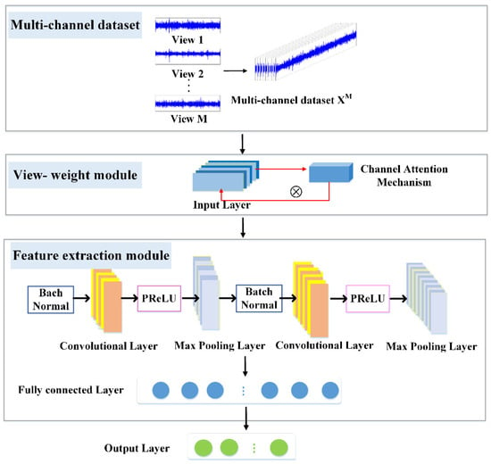
Figure 1. Framework of the CAM_MCFCNN model.

3.1. Multi-Channel Dataset

Different from the traditional mode of concatenating multi-view information or forming a two-dimensional matrix, this study is inspired by the color image channel, and without destroying the multi-view data space structure, the one-dimensional time domain signals of multiple views are jointly constructed into a dataset with multi-channel attributes. The dataset of channel attributes associates the information expressing the operating state in multiple directions within the corresponding time, and the fusion method is more natural.

First, the data from multiple views are preprocessed. The monitoring of the sensor in each direction is defined as a viewing angle, assuming that there are M viewing angles, and the length of the data of each viewing angle is L, and then the samples of the M viewing angles at the corresponding time are constructed into a dataset with M channels.

Then the multi-channel dataset is used as the input of the CAM_MCFCNN model. Different from the traditional fault diagnosis method based on the CNN model, the CAM_MCFCNN model has multiple input channels in the input layer, each channel is independent of each other, and its input corresponds to one dimension of the multi-channel dataset.

3.2. View-Level Weight Module

Considering the difference in importance of multi-view data, it is not enough to directly fuse the data, and an effective feature fusion mechanism is needed. The core of the Channel Attention Mechanism (CAM) is to model and learn the importance of different channel features according to the relationship between channel features. This study utilizes the CAM [20] module to allocate resources to calibrate the importance of each view. The model structure is shown in Figure 2. which mainly includes three parts: dimension compression module, excitation module and re-weighting.

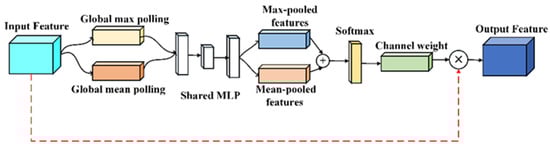
Figure 2. Architecture of the CAM model.

It is assumed that the input of the model is $x^v$, and $v$ represents the number of channels. The CAM model gets the weight vector of each channel through squeezing and excitation, and then maps it to the original feature channel to realize the selection of channel importance. The specific operation process is as follows:

(1)

Squeeze: The CAM compresses feature maps along channel dimensions through global maximum pooling and global average pooling to obtain the global feature representation of each feature map and perceive the feature representation of each channel from a global perspective [21]. The average pooling feature and the maximum pooling feature are represented by $F_{avg}^v=AvgPool(x^v)$ and $F_{\max }^v=MaxPool(x^v)$.

(2)

Excitation: In the excitation operation, $F_{avg}^v$ and $F_{\max }^v$ are respectively sent into a two-layer neural network with a bottleneck structure to model the correlation between different feature channels and generate weights for each feature channel. MLP consists of two convolution layers, each of which uses a 1 × 1 convolution kernel to extract the relationship features between channels. The input and output of MLP are consistent through scaling parameter R. Then, the two features obtained are added together to obtain the weight coefficient $u^v$ through an activation function. The whole process is represented as follows:

$$\begin{array}{cc}{u}^v& =\sigma (MLP(F_{avg}^v)+MLP(F_{\max }^v))\hfill \\ & =\sigma (w_1(f(w_0(F_{avg}^v)))+w_1(f(w_0(F_{\max }^v))))\end{array}$$

(1)

where $f$ and $\sigma$, respectively, represent the ReLU activation function and sigmoid function, and $w_0$ and $w_1$, respectively, represent the convolution kernel parameters in MLP. The value $u^v$ represents the weight information of the $v$th channel, i.e., $1\times 1\times v$.

(3)

Reweight: The obtained channel weight information $u^v$ is mapped to the corresponding channel feature, and the original input feature $x^v$ is recorrected to obtain a feature map ${\tilde{x}}^v$ with channel attention for further fault diagnosis.

$${\tilde{x}}_{}{}^v=x^v\otimes u^v$$

(2)

It has been widely pointed out in the literature that not all views of data contribute equally to the fault diagnosis task, so this study applies different weights to the reconstruction error for multiple views.

The loss function of Equation (1) is modified from the original sigmoid function to the softmax function, so that the weight range representation is changed from the original two values of 0 or 1 to the range of [0, 1].

3.3. Feature Extraction Module

After characterizing the view weights, feature extraction is performed on them. Different from the traditional fault diagnosis method based on the CNN model, the first convolution layer of the CAM_MCFCNN model first extracts the features within the channel, and then extracts the features between the channels. The process of extracting features from multi-channel input by the first convolution layer can be expressed as:

$$\begin{array}{l}fe{a}_k^{L1}=Conv(CAM(x^1,x^2,\dots ,x^v))\\ \hspace{1em}\hspace{1em}\hspace{0.33em}=f({\displaystyle \sum _{v=1}^M{\displaystyle \sum _{j=1}^N{\tilde{x}}_{i,j}^v}}\ast w_k^{L1}+b_{}{}^{L1})\end{array}$$

(3)

where $j$ represents the length of the input feature map; $M$ represents the number of input channels, that is, the total number of views; ${\tilde{x}}_{i,j}^v$ represents the ith sample of the input of the $v$th channel of the first input layer; $w_k^{L1}$ represents the weight of the $k$th convolution kernel of the first convolution layer L1; and the corresponding generated feature map is represented by $fe{a}_k^{L1}$.

After the convolution operation, the PReLU function [22] is used as the activation function to non-linearly transform the output value of each convolution. Different from the commonly used ReLU function, the PReLU function adds an adaptive slope a on the negative half axis. When the input value is negative, the non zero activation value is output, which improves the zero-gradient problem of the negative half of ReLU and makes the network respond to both positive and negative directions. The PReLU function is well adapted to the reciprocal fluctuation nature of vibration signals and reduces information loss [23]. The expression of the PReLU activation function is as follows:

$$P\mathrm{Re}LU(fe{a}_i)=\left\{\begin{array}{l}fe{a}_i\\ a_{i}fe{a}_i\end{array}\right.\begin{array}{c}if\begin{array}{cc}fe{a}_i>0& \end{array}\\ if\begin{array}{cc}fe{a}_i<0& \end{array}\end{array}$$

(4)

where $fe{a}_i$ represents the feature of the ith channel, and $a_i$ is learnable parameter.

3.4. Diagnosis Procedure

The fault diagnosis process of the CAM_MCFCNN model is shown in Figure 3, which mainly includes the following steps:

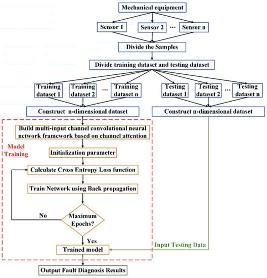
Figure 3. Flowchart of the proposed method.

(1)

Building a multi-channel dataset: Sensors are deployed at different positions of the mechanical equipment to collect the operating status under different operating conditions, and each monitoring direction is a view. Firstly, the multi-view data is preprocessed and divided into samples with a certain length d. Let ${\{X_i^{(v)}\in R^{N\times d}\}}_{v=1}^M$ denote the $N$ samples in the $M$ views, and $X_i^{(v)}\in R^{N\times d^{}}$ denote the $i$ samples in the $v$ view. Then, the samples from M views are constructed into a sample set $X_{M\times N\times d}$ with M-dimensional channels, and a training set and a test set are constructed according to a certain proportion, which are used for model training and testing respectively.

(2)

Constructing the CAM_MCFCNN model: Determine the structure and parameters of the model according to the input and output dimensions of the multi-channel dataset.

(3)

Model training stage: The training samples are used to train the CAM_MCFCNN model. Training stops when the number of iterations reaches the requirement, and a pre-trained model is obtained.

(4)

Model testing stage: After training, the test samples are input into the trained model to get the diagnosis results.

4. Experimental Verification and Analysis

The effectiveness of the model is carried out on the planetary gearbox experimental dataset and compared with the existing information fusion methods. In order to avoid random sampling errors, all experiments are tested 10 times to ensure the reliability of the results.

4.1. Description of Experimental Equipment

The experimental system of the planetary gearbox is shown in Figure 4a. The system was composed of an operating console, drive motor, elastic coupling, helical gearbox, planetary gearbox, magnetic powder brake, and isolation floor. The operating console changed the speed of the motor and the damping coefficient of the brake by adjusting the voltage and current values. The drive motor provided the power source, which was transmitted to the magnetic particle brake through the helical gearbox, elastic coupling and planetary gearbox. The fault simulation experiment was conducted in the planetary gearbox, which consisted of an 18-tooth sun gear, three 27-tooth planetary gears, a planet carrier and a 72-tooth ring gear; the internal structure is shown in Figure 4b. The sun gear connected with the input shaft was surrounded by three planetary gears, the planetary gears revolved around the sun gear while rotating, and the planetary gears meshed with the sun gear and the ring gear at the same time. In the experiment, five wear faults of different severity were simulated on a planetary gear, five different health states of the planet gears were simulated, namely, normal state, single tooth wear, two teeth wear, three teeth wear and all teeth wear. The planet gears in the five health states are shown in Figure 4d–h.

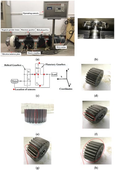
Figure 4. (a) Structure of the planetary gearbox test rig, (b) The internal structure of planetary gearbox, (c) locations of five accelerometer sensors, (d) normal state, (e) single tooth wear, (f) two teeth wear, (g) three teeth wear, and (h) all teeth wear.

Considering the special structure of the planetary gearbox and the influence of the change of the vibration transmission path, during the experiment, the acceleration sensors were respectively arranged at five different plane positions on the surface of the planetary gearbox according to the experimental scheme in [24]. The two three-direction sensors were mounted on both sides of the planetary gearbox body to measure acceleration in (x, y, z) directions; two one-direction sensors were installed above the inner bearing seat of the input and output shafts of the planetary gearbox to measure the acceleration in z direction. A one-direction sensor was placed above the center of the planetary gearbox top cover. The acceleration sensor information is listed in Table 1. The monitoring point positions of each sensor are shown in Figure 4c. In each failure mode, the motor was tested once at 1200 rpm, 1500 rpm and 600 rpm (corresponding loads are 0.3 HP, 0.5 HP and 1 HP, respectively). In each test, the sampling frequency of the acquisition system for all sensors is set to 20.4 kHz, and the sampling time was 30 s.

Table 1. The acceleration sensor information used in the experiment.

Number	Measuring Point Position	Model	Direction	Sensitivity
1	Outer side of planetary gearbox body	CA-YD-3152	X	2.01
			Y	1.99
			Z	1.92
2	Inner side of planetary gearbox body	CA-YD-3152	X	2.03
			Y	2.09
			Z	2.01
3	Inner bearing seat of planetary wheel output shaft	YD-36D	Z	1.88
4	Inner bearing seat of planetary wheel input shaft	YD-36D	Z	1.98
5	Center of planetary gearbox top cover	YD-36D	Z	1.92

4.2. Multi-View Data Acquisition

During the experiment, each monitoring direction of the three-direction sensor was regarded as a view. Therefore, five sensors obtained nine data views. The time-domain waveform of the vibration signal of the planetary gear all teeth wear simultaneously collected by five different acceleration sensors at nine views when the rotation speed was 1500 rpm is shown in Figure 5. As can be seen from the figure, the time-domain waveforms of the first, fourth and seventh views were very similar in time-domain waveforms, indicating that the information from different views had a certain consistency and redundancy. However, the second, fifth and seventh views show relatively large differences in amplitude and time-domain waveform, indicating that there were certain differences and complementarities between the information of different views. Therefore, it can be predicted that the amplitudes of the vibration signals monitored from different views were different, and the information contained in these vibration signals was different. Combining multi-view data can provide more information for fault diagnosis.

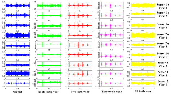
Figure 5. Raw vibration signals of five health states of planetary gearbox collected by multi-sensors at 1500 rotation speed.

4.3. Experimental Dataset

After the completion of the data acquisition, a multi-channel dataset was constructed. There were 600 samples for each health state in each view, and 3000 samples for five health states, each sample consisted of 1024 points. The samples of nine views were divided into three datasets according to the motor speed. Datasets A, B and C were vibration signals obtained at constant rotational speeds of 1200 rpm, 1500 rpm and 600 rpm, respectively. Each dataset had nine channels, and the size of each channel was 1 × 1024. Then, 20% samples of each health state were randomly selected from the datasets A, B, and C to form the dataset D, which was used to evaluate the stability of the model at the mixing speed. In dataset D, data with the same health status from different rotational speeds were considered as the same type, so the dataset contains five different health conditions at three different motor speeds. Each dataset was divided into a training set and a test set according to the ratio of 8:2, as shown in Table 2.

Table 2. The training set and test set at different speed.

Dataset	Label	Describe the Fault State	Number of Samples per View	Numeber of Views
A/B/C/D	0	Normal	600/600/600/200	9
	1	Single tooth wear	600/600/600/200	9
	2	Two teeth wear	600/600/600/200	9
	3	Three teeth wear	600/600/600/200	9
	4	All teeth wear	600/600/600/200	9

4.4. Model Parameter Settings

The network structure and parameter settings of the CAM_MCFCNN model are presented in Table 3, where R is the scaling factor, C represents the number of convolutional kernels, KS stands for the convolution kernel size, S is the sliding step of the convolution kernel. The number of channels of the input module was set according to the number of sensor channels deployed in the experiment. In the feature extraction module, since the vibration signal is one-dimensional, in order to obtain a larger sensing field, a larger size convolution kernel was used. Other parameters of the model were set according to relevant experience. Specifically, the model used a fixed learning rate, which was set to 0.0015. The minimum batch is 100, and the number of iterations is 100.

Table 3. Module parameters setup of of CAM_MCFCNN model.

Module	Layer	Parameters	Output Size
Input	Input Layer	Channel = 9	[9 × 1 × 1024]
View-level weight	Global average Pooling	None	[9 × 1]
	Global max Pooling	None	[9 × 1]
	Convolutional Layer 1	C = 18, KS = 1	[18 × 1]
	Convolutional Layer 2	R = 1/2, C = 9, KS = 1	[9 × 1]
Feature extraction	Convolutional Layer	C = 20, KS = 9, S = 3	20 × 1 × 339
	Max pooling Layer	Pool size = 2	20 × 1 × 169
	Convolutional Layer	C = 40, KS = 9, S = 3	40 × 1 × 54
	Max pooling Layer	Pool size = 2	40 × 1 × 27
	Fully connection Layer	Hidden Nodes = 100	100 × 1
Output	Fully connection Layer	Hidden Nodes = 5, activation = Softmax	[5 × 1]

4.5. Comparative Analysis

4.5.1. Comparison between Single-Channel Fault Diagnosis Methods and Multi-Channel Fault Diagnosis Methods

In this section, the data of each view was input into the single-channel CNN model in the same way, and the comparison experiments were carried out with the proposed method. Each method was repeated 10 times, the diagnostic results of the model on test sets A, B and C are shown in Figure 6. As can be seen from the figure, the diagnostic accuracy of the CAM_MCFCNN model basically reached 100%. The diagnostic accuracy of the single-channel CNN model was affected by the view positon. The signal quality was related to the view position to a certain extent, which determines the number of fault features contained in the signal. Therefore, the fusion of multi-view information could provide more comprehensive and accurate information for the fault diagnosis of the gearbox.

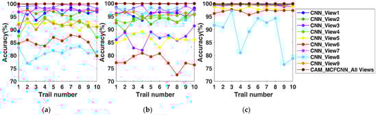
Figure 6. Diagnostic accuracy of ten experiments with single-channel convolutional neural networks (CNN) based on single-view data and CAM_MCFCNN based on multi-view data on test sets A (a), B (b), and C (c), respectively.

The average test accuracy, standard deviation and average training time of the model in ten trials were shown in Table 4. As can be seen from the table, the average diagnostic accuracy of the CAM_MCFCNN model on different datasets was between 99.87% and 99.95%, while the average diagnostic accuracy of the single-channel CNN model was between 81.10% and 99.58%. The average test accuracy of the single-channel CNN based on view 1 and view 9 was between 96.12% and 99.58%. Although they had reached acceptable test accuracy, the standard deviation of the single-channel CNN model was much larger than that of the CAM_MCFCNN model. In addition, compared with the single-channel CNN model, The multi-channel structure of the CAM_MCFCNN model had little effect on the training time while improving the accuracy of diagnosis.

Table 4. Average testing accuracy, standard deviation, and model training average time of single-channel CNN data and CAM_MCFCNN.

View Data	Diagnosis Strategies	Average Testing Accuracy ± Standard Deviation (%)
		A	B	C
View 1	Separate diagnosis	96.11 ± 2.78	96.02 ± 1.26	99.57 ± 0.16
View 2	Separate diagnosis	96.74 ± 0.83	93.48 ± 1.91	99.88 ± 0.14
View 3	Separate diagnosis	97.50 ± 0.85	86.75 ± 2.81	99.37 ± 0.35
View 4	Separate diagnosis	91.68 ± 2.53	93.97 ± 0.98	99.78 ± 0.18
View 5	Separate diagnosis	92.02 ± 1.03	86.27 ± 1.69	98.12 ± 0.53
View 6	Separate diagnosis	85.15 ± 2.30	77.78 ± 2.50	96.97 ± 0.63
View 7	Separate diagnosis	99.00 ± 0.66	97.62 ± 1.30	99.58 ± 0.21
View 8	Separate diagnosis	81.10 ± 1.98	97.02 ± 1.50	88.65 ± 7.23
View 9	Separate diagnosis	92.15 ± 1.40	95.72 ± 0.67	99.43 ± 0.20
All views	Collaborative diagnosis	99.95 ± 0.06	99.87 ± 0.12	99.92 ± 0.07

In order to more clearly explain the recognition effect of the model on each fault category of the test set, the best diagnostic results of the seventh view data with the best signal quality were selected to compare with the worst diagnostic results after multi-view fusion, as shown in Figure 7. The best diagnosis results of the single-channel CNN model on the three test sets are shown in Figure 7(a1–a3). Except for test set C, the accuracy of the single-channel CNN model on test sets A and B was lower than that of the CAM_MCFCNN model. On test set A, the diagnosis accuracy was 99.7%; two samples of three teeth wear states were misclassified as single tooth wear. On test set B, one sample of three teeth wear was misdiagnosed as two teeth wear, and three samples of normal state were misdiagnosed as single tooth wear. The worst diagnosis results of the CAM_MCFCNN model in the three test sets are shown in Figure 7(b1–b3). In test sets A and C, the diagnostic accuracy of the proposed method is 99.8%, and the misdiagnosis rate is 0.2%. In test set B, the diagnostic accuracy of the proposed method is 99.7%, and the misdiagnosis rate is 0.3%. Except for two samples of two teeth wear were misdiagnosed as normal, the classification accuracy of the other four states reached 100%. However, it is worth noting that the worst diagnosis results of the proposed method of multi-view data fusion were compared with the best diagnosis results of the single-channel CNN model of single-view data.

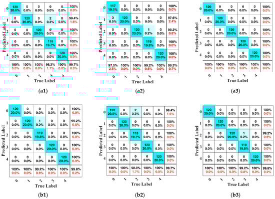
Figure 7. Confusion matrices of five wear fault conditions. (a1–a3) are the confusion matrices of the single-channel CNN method in testing datasets A, B, and C, respectively. (b1–b3) are the confusion matrices of the CAM_MCFCNN method in testing datasets A, B, and C, respectively.

In order to further verify whether the proposed model can learn discriminative features, t-SNE [25] was used to project the features learned by the fully connected layer of the CAM_MCFCNN model on the multi-channel dataset into the two-dimensional space for visualization and compared with the features learned by the single-channel CNN model on the ninth view dataset. The corresponding visualization results are shown in Figure 8. Each point in the figure represented a sample, and different colors represented different health states of the planet wheels.

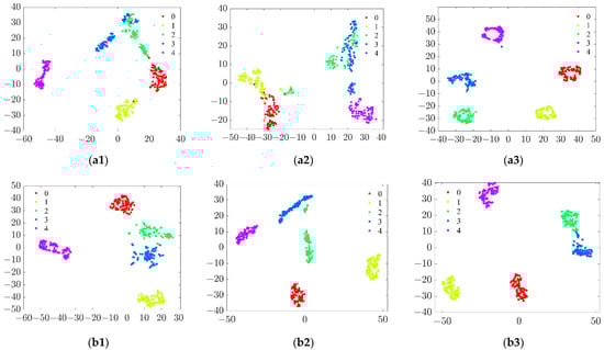
Figure 8. T-SNE visualization of features learned in the fully connected layer: (a1–a3) indicate the features of single-channel CNN from testing datasets A, B, and C; (b1–b3) indicate the features of CMA_MCFCNN from testing datasets A, B, and C.

As can be seen from the figure, in terms of the feature distribution of the fully connected layer, the features of the same health state learned by the CAM_MCFCNN model show better clustering performance within the class, while different health states show better separation performance. The single-channel CNN model shows good features separation ability on the test set C, but on the test dataset A, the features of two teeth wear and three teeth wear overlap. On the test dataset B, except that the features of all teeth wear were clustered together, there was overlap between three teeth wear and two teeth wear, normal state and single tooth wear. This shows that the CAM_MCFCNN model has better discriminative features than the features learned by the single-channel CNN model.

4.5.2. Applicability of CAM_MCFCNN under Limited Training Sample Conditions

Aiming at the problem of the difficulty in obtaining the fault data of a planetary gearbox in actual production, the classification performance of the proposed model was evaluated when the training samples were insufficient. The proportion of training samples was gradually reduced from 80% to 10%, and the model was repeated 10 times on the training set obtained at each proportion. The average diagnostic results of the single-channel CNN and the CAM_MCFCNN model on the test set are shown in the Figure 9.

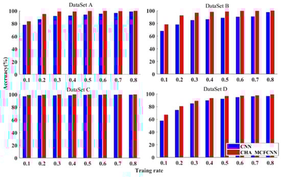
Figure 9. The average diagnostic results of single channel CNN and CAM_MCFCNN model on the test sets under limited training sample conditions.

It can be observed from the figure that in the four datasets, compared with the single-channel CNN model, the CAM_MCFCNN model significantly improved the classification accuracy in both constant-speed and mixed-speed instances with fewer training samples. In the constant running datasets A, B and C, when 20% of the samples were used for training, the average diagnostic accuracy of the CAM_MCFCNN model was 94.98%, 92.33% and 99.44%, respectively. However, the average diagnostic accuracy of the single-channel CNN model was 86.65%, 78.08% and 98.08%, respectively. For dataset D, containing samples of different rotational speeds, when 10% of the samples were used for training, the diagnostic accuracy of both models was not ideal. However, when the training samples increased to 40%, the average diagnostic accuracy of the CAM_MCFCNN model increased to 93.18%. The accuracy of the single-channel CNN model was 89.61%. The experimental results show that the proposed approach is effective and has a certain value in the industrial environment where training samples are scarce.

4.5.3. Comparison with Other Fault Diagnosis Methods

In order to verify that the CMA-MCFCNN model has certain advantages in recognition performance compared with the current multi-view information fusion algorithms, four multi-view information fusion models were selected for comparison, two models were based on data-level fusion, and the other two models were based on feature-level fusion and decision-level fusion. The input data of the method used for comparison were as follows:

(1)

A DCNN model with large convolution kernel size was proposed by Jing et al. [10]., using raw vibration signal as input. In the experiment, 114 data points intercepted in the corresponding time points of the vibration signals from nine views were connected in series to form a sample with a length of 1026.

(2)

Xia et al. [11] proposed a two-dimensional CNN model (2DCNN) composed of two groups of “convolutional layers + pooling layers” stacked, and the vibration signals of nine views were stacked row by row to form a two-dimensional matrix as the input of the model. In the experiment, the samples of nine groups of vibration signals were stacked row by row to form a matrix size of 9 × 1024.

(3)

Xie et al. [15] proposed a feature-level fusion fault diagnosis method (CNN_EMD) based on CNN and EMD. This method fused 80 CNN features, 11 time domains and EMD features, and then trained a sofmax classifier for fault diagnosis. In the experiment, a fast Fourier transform, time-domain feature extraction and empirical mode decomposition were performed on the vibration signals collected from the seventh view, and then the frequency spectrum obtained by the Fourier transform was input into the CNN model.

(4)

Li et al. [18] proposed an ensemble deep Convolutional Neural Network model with improved D-S evidence (IDSCNN), taking the root mean square (RMS) maps from the FFT (Fast Fourier Transformation) features of the vibration signals as the input of model. In the experiment, FFT was performed on the vibration signals at the seventh and second view, respectively.

The comparison results of all methods are listed in Table 5. The average diagnostic accuracy of the proposed CAM_MCFCNN model on the three constant-speed datasets A, B and C is 99.95%, 99.87% and 99.92%, respectively, and the average diagnostic accuracy on the mixed-speed dataset D is 98.89%. Compared with the second-highest DCNN, the diagnostic accuracy of the CAM_MCFCNN model on the four datasets was improved by 7.3%, 6.04%, 1.21% and 7.06%, respectively. The CNN_EMD model had the lowest accuracy. The possible reason for this is that the hand-extracted features were not adapted to the fault mode of this study. The diagnosis accuracy of the CNN_EMD model had the worst performance on dataset D, which indicates that the features are not sensitive to speed.

Table 5. Performance analysis of comparative methods.

Model	The Average Test Accuracy ± Standard Deviation (%)				Average Training Time (min)	Number of Parameters
	DataSet A	DataSet B	DataSet C	DataSet D
DCNN	92.65 ± 1.49	93.83 ± 1.84	98.71 ± 0.67	91.83 ± 1.64	10.6 (CPU)	≈258318
2DCNN	84.35 ± 3.81	77.92 ± 3.35	87.11 ± 3.91	83.92 ± 3.24	8 (CPU)	≈177615
CNN_EMD	82.11 ± 2.45	75.59 ± 3.21	84.65 ± 2.09	70.16 ± 2.30	15 (CPU)	≈654360
IDSCNN	91.91 ± 1.30	92.37 ± 2.69	96.41 ± 1.25	90.45 ± 2.63	15 (GPU)	≈532650
Proposed method	99.95 ± 0.06	99.87 ± 0.12	99.92 ± 0.07	98.89 ± 0.05	6.72 (CPU)	≈117705

In addition, this study also analyzed and compared the model training time and parameters of each method. IDSCNN adopts the method of ensemble branch network, which suffers from high complexity during the training process as well as testing. Compared with other methods, the proposed CAM_MCFCNN model has a simple structure, fewer parameters and a shorter training time. The experimental results show that the proposed multi-view information fusion model with view-level weights is effective.

4.5.4. Discussion

(1)

Through the comparative analysis of the single-view information model CNN and the multi-view information fusion model CAM_MCFCNN, it can be concluded that the CAM_MCFCNN model has improved diagnostic accuracy and stability in both constant-speed and mixed-speed datasets, which indicates that comprehensive utilization of multi-view information can more comprehensively reflect the equipment operation status and improve the reliability of status monitoring and fault diagnosis. From the feature visualization results, it can be seen that the features learned by the CAM_MCFCNN model are more compact and centralized, and the clustering is more obvious. Compared with the features learned by the single-view CNN model, the features learned by the CAM_MCFCNN model have better discriminability, which can effectively improve the performance and accuracy of the fault diagnosis method.

(2)

Compared with other multi-view information fusion methods, the CAM_MCFCNN model achieved the best performance, which further proves that the weight scheme based on the attention mechanism is effective. At the same time, the CAM_ MCFCNN model can automatically learn the weight of each perspective, which saves labor and is easier to promote and apply in practice.

5. Conclusions and Future Work

Aiming at the problems of uncertainty and unreliability in fault diagnosis methods based on single-view information, this paper proposes a multi-view information fusion CAM_MCFCNN model with view-level weights. The proposed model integrates multi-view information at the data layer, and can learn the weight of each view, so that the model pays more attention to important features and fault-sensitive views during the training process, and integrates information from different views more reasonably. The experimental results on the planetary gearbox fault dataset show that the diagnosis accuracy and feature learning ability of the CAM_MCFCNN model are better than that of the single-channel CNN model. Especially in the case of small samples, the diagnosis accuracy of the CAM_MCFCNN model on the constant-speed dataset was significantly higher than that of the single-channel CNN model. On the mixed-speed dataset, the CAM_MCFCNN model has good robustness, and the accuracy can reach more than 93% when the proportion of training samples is 40%. At the same time, compared with other multi-view information fusion algorithms, the proposed model can obtain good diagnostic accuracy on different datasets.

Due to the limitations of experimental conditions, this paper uses isomorphic multi-view data for experiments. In the future, different types of sensors will be used to monitor the state of mechanical equipment, and fault diagnosis methods based on heterogeneous multi-view information fusion will be studied.

References

- Diez-Olivan, A.; Del Ser, J.; Galar, D.; Sierra, B. Data fusion and machine learning for industrial prognosis: Trends and perspectives towards Industry 4.0. Inf. Fusion 2019, 50, 92–111. [Google Scholar] [CrossRef]
- Huang, R.; Li, J.; Li, W.; Cui, L. Deep Ensemble Capsule Network for Intelligent Compound Fault Diagnosis Using Multisensory Data. IEEE Trans. Instrum. Meas. 2020, 69, 2304–2314. [Google Scholar] [CrossRef]
- Xu, C.; Guan, Z.; Zhao, W.; Niu, Y.; Wang, Q.; Wang, Z. Deep Multi-View Concept Learning. In Proceedings of the Twenty-Seventh International Joint Conference on Artificial Intelligence IJCAI-18, Stockholm, Sweden, 9–19 July 2018. [Google Scholar]
- Xu, C.; Tao, D.; Xu, C. A Survey on Multi-view Learning. arxiv 2013, arXiv:1304.5634. [Google Scholar]
- Shao, H.; Lin, J.; Zhang, L.; Galar, D.; Kumar, U. A novel approach of multisensory fusion to collaborative fault diagnosis in maintenance. Inf. Fusion 2021, 74, 65–76. [Google Scholar] [CrossRef]
- Wang, X.; Feng, Y.; Song, R.; Mu, Z.; Song, C. Multi-Attentive Hierarchical Dense Fusion Net for Fusion Classification of Hyperspectral and LiDAR Data. Inf. Fusion 2022, 82, 1–18. [Google Scholar] [CrossRef]
- Chehade, A.; Song, C.; Liu, K.; Saxena, A.; Zhang, X. A data-level fusion approach for degradation modeling and prognostic analysis under multiple failure modes. J. Qual. Technol. 2018, 50, 150–165. [Google Scholar] [CrossRef]
- Long, Z.; Zhang, X.; Zhang, L.; Qin, G.; Huang, S.; Song, D.; Shao, H.; Wu, G. Motor fault diagnosis using attention mechanism and improved adaboost driven by multi-sensor information. Measurement 2021, 170, 108718. [Google Scholar] [CrossRef]
- Huang, M.; Liu, Z.; Tao, Y. Mechanical fault diagnosis and prediction in IoT based on multi-source sensing data fusion. Simul. Modell. Pract. Theory 2020, 102, 101981. [Google Scholar] [CrossRef]
- Jing, L.; Wang, T.; Zhao, M.; Wang, P. An Adaptive Multi-Sensor Data Fusion Method Based on Deep Convolutional Neural Networks for Fault Diagnosis of Planetary Gearbox. Sensors 2017, 17, 414. [Google Scholar] [CrossRef]
- Xia, M.; Li, T.; Xu, L.; Liu, L.; de Silva, C.W. Fault Diagnosis for Rotating Machinery Using Multiple Sensors and Convolutional Neural Networks. IEEE/ASME Trans. Mechatron. 2017, 23, 101–110. [Google Scholar] [CrossRef]
- Azamfar, M.; Singh, J.; Bravo-Imaz, I.; Lee, J. Multisensor data fusion for gearbox fault diagnosis using 2-D convolutional neural network and motor current signature analysis. Mech. Syst. Signal Process. 2020, 144, 106861. [Google Scholar] [CrossRef]
- Chen, Z.; Li, W. Multisensor feature fusion for bearing fault diagnosis using sparse autoencoder and deep belief network. IEEE Trans. Instrum. Meas. 2017, 66, 1693–1702. [Google Scholar] [CrossRef]
- Shao, S.; Yan, R.; Lu, Y.; Wang, P.; Gao, R.X. DCNN-Based Multi-Signal Induction Motor Fault Diagnosis. IEEE Trans. Instrum. Meas. 2020, 69, 2658–2669. [Google Scholar] [CrossRef]
- Xie, Y.; Zhang, T. Fault Diagnosis for Rotating Machinery Based on Convolutional Neural Network and Empirical Mode Decomposition. Shock Vib. 2017, 2017, 3084197. [Google Scholar] [CrossRef]
- Li, H.; Huang, J.; Ji, S. Bearing Fault Diagnosis with a Feature Fusion Method Based on an Ensemble Convolutional Neural Network and Deep Neural Network. Sensors 2019, 19, 2034. [Google Scholar] [CrossRef]
- Li, H.; Huang, J.; Yang, X.; Luo, J.; Zhang, L.; Pang, Y. Fault Diagnosis for Rotating Machinery Using Multiscale Permutation Entropy and Convolutional Neural Networks. Entropy 2020, 22, 851. [Google Scholar] [CrossRef]
- Li, S.; Liu, G.; Tang, X.; Lu, J.; Hu, J. An Ensemble Deep Convolutional Neural Network Model with Improved D-S Evidence Fusion for Bearing Fault Diagnosis. Sensors 2017, 17, 1729. [Google Scholar] [CrossRef]
- Fu, Y.; Chen, X.; Liu, Y.; Son, C.; Yang, Y. Gearbox Fault Diagnosis Based on Multi-Sensor and Multi-Channel Decision-Level Fusion Based on SDP. Appl. Sci. 2022, 12, 7535. [Google Scholar] [CrossRef]
- Woo, S.; Park, J.; Lee, J.Y.; Kweon, I.S. CBAM: Convolutional Block Attention Module; Springer: Cham, Switzerland, 2018; pp. 3–19. [Google Scholar]
- He, K.; Zhang, X.; Ren, S.; Sun, J. Delving Deep into Rectifiers: Surpassing Human-Level Performance on ImageNet Classification. In Proceedings of the Conference on Computer Vision and Pattern Recognition CVPR, Boston, MA, USA, 7–12 June 2015; IEEE Computer Society: New York, NY, USA, 2015. [Google Scholar]
- Zhao, D.; Liu, S.; Zhang, H.; Sun, X.; Wang, L.; Wei, Y. Intelligent Fault Diagnosis of Reciprocating Compressor Based on Attention Mechanism Assisted Convolutional Neural Network Via Vibration Signal Rearrangement. Arab. J. Sci. Eng. 2021, 46, 7827–7840. [Google Scholar] [CrossRef]
- Liu, S.; Huang, J.; Ma, J.; Luo, J. SRMANet: Toward an Interpretable Neural Network with Multi-Attention Mechanism for Gear box Fault Diagnosis. Sciences 2022, 12, 8388. [Google Scholar] [CrossRef]
- Feng, Z.; Zuo, M.J. Vibration signal models for fault diagnosis of planetary gearboxes. J. Sound Vib. 2012, 331, 4919–4939. [Google Scholar] [CrossRef]
- Laurens, V.D.M.; Hinton, G. Visualizing Data using t-SNE. J. Mach. Learn. Res. 2008, 9, 2579–2605. [Google Scholar]
Publisher’s Note: MDPI stays neutral with regard to jurisdictional claims in published maps and institutional affiliations. |
© 2022 by the authors. Licensee MDPI, Basel, Switzerland. This article is an open access article distributed under the terms and conditions of the Creative Commons Attribution (CC BY) license (https://creativecommons.org/licenses/by/4.0/).