Learning Motion Constraint-Based Spatio-Temporal Networks for Infrared Dim Target Detections

Abstract

Efficient infrared dim object detection has been challenged by low signal-to-noise ratios (SNRs). Traditional methods rely on the gradient difference and fixed-parameter model. These methods fail to adapt to sophisticated and variable situations in the real world. To tackle the issue, a deep learning method based on the spatio-temporal network is proposed in this paper. The model is established by the Convolutional Long Short-Term Memory cell (Conv-LSTM) and the 3D Convolution cell (3D-Conv). It is trained to learn the motion constraint of moving targets (spatio-temporal constraint module, called STM) and to fuse the multiscale local feature between the target and background (deep spatial features module, called DFM). In addition, a variable interval search module (state-aware module, called STAM) is added to the inference. The submodule decides to conduct a global search for images only if the target is lost due to fast motion, uncertain obstruction, and frame loss. Comprehensive experiments indicate that the proposed method achieves better performance over all baseline methods. On the mid-wave infrared datasets collected by the authors, the proposed method achieves a 95.87% detection rate. The SNR of the dataset is around 1–3 dB, and the background of the sequence includes sky, asphalt road, and buildings.

1. Introduction

The Infrared Search and Tracking (IRST) system based on the thermal radiation principle has superiority in terms of favorable concealment and night monitoring. With the fast-growing development of unmanned aerial vehicles (UAVs), the remote monitoring and early warning of the IRST have drawn substantial attention. Due to the long-range distance, the UAV’s image appears with very few pixels and fuzzy texture in the infrared image [1]. Worse still, the complicated background may introduce random noise. The detection of robust infrared dim targets, therefore, is still a challenging task.

Researchers developed various algorithms to solve the problem. Specifically, the involved methods can be divided into two types: traditional methods and deep learning methods.

A. Traditional methods

Traditional methods can be further classified into those that are single-frame-based and multiple-frame-based. Single-frame-based methods are mainly based on the edge gradient between the background and the target. Many effective algorithms have been proposed in recent years. When considering morphological filtering, Rang et al. [2] adopted omnidirectional morphological filters to detect small targets. However, the method cannot avoid the disadvantage of the fixed parameter. Inspired by the mathematical theory, Guan et al. [3] improved the popular infrared patch-tensor (IPT) model with a non-convex tensor rank surrogate merging tensor nuclear norm (TNN) and the Laplace function. The method requires complex iterative computation, which makes it difficult for real-time detection. Zhang et al. [4] figured out that the adjacent region of a dim target holds a Mexican hat distribution. Their experiments indicate that direct detection would degrade performances when the background becomes complicated. Moreover, there are many ways to consider the Human Visual System (HVS). According to the HVS, Rao et al. [5] proposed a weighted local coefficient of variation (WLCV) for small target detection. Pan et al. [6] computed the diagonal grey-level difference to suppress the background. Wu et al. [7] used a fixed-size sliding window to detect different target sizes, which is called the Double-Neighborhood Gradient Method (DNGM). Nevertheless, the above-discussed algorithms are based on the hypothesis of the local maximum. They become very poor when the SNR decreases rapidly.

The traditional multiple-frame-based algorithms are designed to capture the motion trajectory to detect the target. They depend on rigorous mathematical theories. Yang et al. [8] improved the mixture of the Gaussian (MoG) model to describe the noise and select the target via the difference between the target and background in a modified flux density (MFD) method. The method is strictly based on low-rank assumptions leading to impracticability in real applications. Chiman et al. [9] used two optical flow methods (TV-L1 and Brox) with contrast enhancement kernels to detect the moving small target. They consume more computational time to achieve better accuracies. Lvping yue et al. [10] considered using background movement to suppress the background and enhance the foreground. They utilized Pearson’s correlation coefficient and the regional gray level (RGL). Wang et al. [11] addressed the target maneuver by using a general measurement-directed (MD) strategy. Online learning of the target from the observations was achieved. However, the high detection rate depends on the hypothesis of the gray-level distribution. Most multiple-frame methods suppose that the background is uniform, and the motion is slow. They need more computational resources to adapt to the inconsistency of the background and target motion.

As analyzed above, the traditional methods mainly rely on the edge gradient between the background and the target. Typical single-frame methods perform well when the background is relatively unitary. However, the result is very sensitive to the bad points, which are blamed for the production defect of the infrared sensors. Widely used multi-frame algorithms take advantage of serial correlations. However, they consume too many computer resources. The calculation of fixed parameters and the sensitivity to bad points limit the effectiveness of traditional algorithms.

B. Deep learning methods

Early methods that relied on gradient operation were gradually surpassed by popular convolutional neural networks. Recent approaches are inclined toward the deep learning model. The R-CNN (Region-CNN, CNN: convolutional neural network) family [12] is used on behalf of the two-stage detector. The candidate region is generated first for classification and regression. The Yolo (You Only Look Once) family [13,14], the SSD (Single Shot MultiBox Detector) [15], and the RetinaNet [16] are representatives of the single-stage detector. In contrast, coordinates and categories regressed directly without candidates. The single-stage methods greatly improve detection speeds. However, their convolution layers are too deep for the dim target. The high-level features are not prominent in long-range infrared frames.

In light of the above problems, researchers have contributed large efforts. Ryu J et al. [17] improved the SSD to fuse infrared gray-temperature data. Still, it is based on a single frame and cannot solve occasional occlusion. Hwa B et al. [18] combines the full convolution regression network (FCRN) with graph matching to achieve robust detection. Meanwhile, they use the optical flow to obtain motion information. Shi M et al. [19] designed an end-to-end model inspired by the denoising autoencoder, which treats the small target as the “noise” and transforms detections into a denoising task. However, it still causes terrible false alarms. Ju M et al. [20] proposed a single-shot detector. It comprises an image filtering module (IFM) and infrared small target detection module (ISTDM). The IFM aims to enhance valid information and suppress noise. The ISTDM is an efficient convolutional neural network for improving small target detection tasks. Kim S et al. [21] focused on applying a deep neural network to classify the proposal regions rather than pre-processing to reduce the false alarm. Liu M et al. [22] attempted to take small infrared target detection as a classifying task. They exploited synthetic data to train the proposed deep-learning network. Their experiments show that the choice of SNR affects the performance of deep networks. Sheng et al. [23] combined Fully Convolutional One-Stage Object Detection (FCOS) with traditional filtering to enhance the target and suppress the background. The method takes multiple frames as the input of the network but the structure remains single-frame-based. Wang et al. [24] employed the Mask R-CNN model and transfer learning to extract the feature of the small target. However, the method ignores the temporal relation of the moving target.

The discussion shows the usefulness of deep learning models. However, they still have interruption risks during detection when applied in practice, such as uncertain occlusion and redundant calculations. To overcome the existing defect and be motivated by the data-driven proposal, a learning motion constraint network is proposed in this paper. The processing flow of the proposed method is illustrated in Figure 1. In the training phase, spatio-temporal features are learned by stacked Conv-LSTM cells (spatio-temporal constraint module, called STM). Then, the multiscale feature fusion is established by 3D-Conv cells (deep spatial features module, called DFM), which could broaden receptive fields and extract more robust features between the target and the background. The last full connection cell generates the network prediction. In the inference phase, a variable interval search strategy called a state-aware module (state-aware module, called STAM) is proposed. It decides that the network searches for global images only if the target is lost due to fast motion, uncertain obstruction, or frame loss. This submodule highly increases the speed of detection.

The contributions made in this paper are summarized below:

• This paper introduces a learning spatio-temporal constraint module based on Conv-LSTM cells. Experiments show that the model could be applied in long-range infrared target detection.
• This paper fuses multiscale features along the temporal dimension, which makes the detection more efficient and robust.
• This paper applies a state-aware module to achieve dynamic switching between local searching and global re-detection.
• Real datasets are employed to evaluate detection speeds and the robustness of the model.

The remainder of this paper is organized as follows. The proposed model and its analysis are demonstrated in Section 2. The performance of the model is evaluated and discussed in Section 3. We provide conclusions in Section 4.

2. Materials and Methods

The details of the proposed method will be discussed in this subsection. Section 2.1 introduces the handling of the time stream and the design of the network. Section 2.2 analyses the online detecting and updating strategy.

2.1. Training Phase

2.1.1. Time Stream Handing

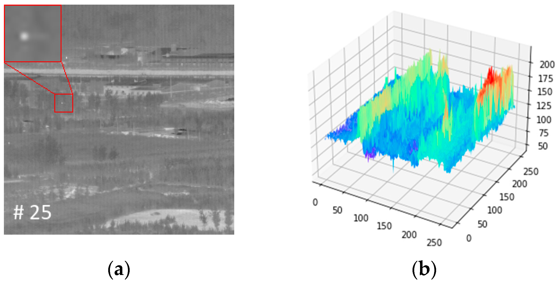
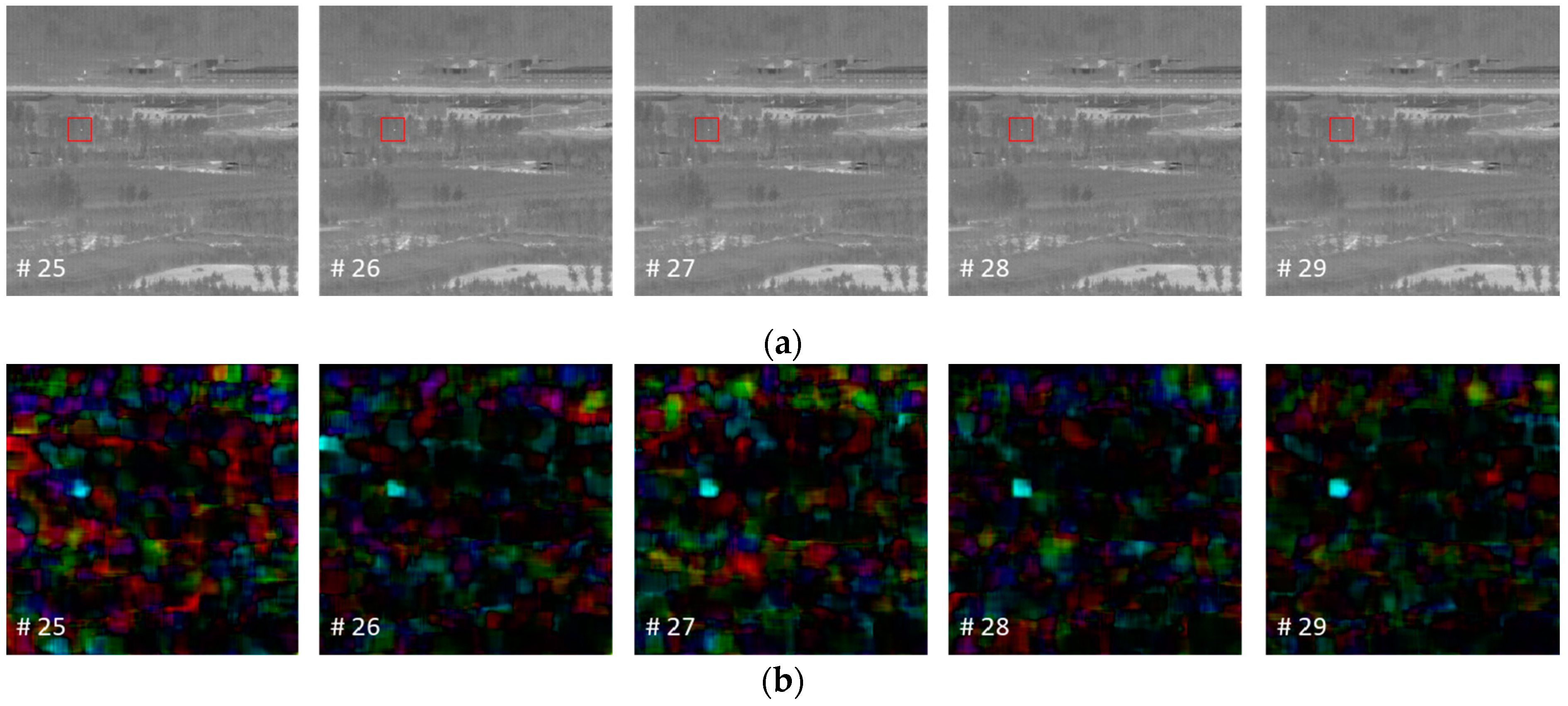
Figure 2a contains a single frame with the common wild environment from the 5000 m distance video, and the target is shown in a red rectangle. Figure 2b is the pixel distribution of the frame. The target occupies only a dozen pixels in the entire image, and its pixel distribution is highly similar to the background clutter due to the lack of color, shape, and texture features. Using only a single frame for small target detection makes detection more difficult. Figure 3a displays five successive frames from the same video, and the targets are shown in red rectangles. Figure 3b represents the movement of pixels in an image sequence by optical flow estimation. Compared to the background, the moving small target has obvious trajectory characteristics. The comparison shows that the target has rich motion information between multiple frames, which can be applied to the detection of moving targets.

The handling of time streams in this paper is shown in Figure 4. The indices i, i − 1…, i − t in the squares indicate the image sequence. When the new frame updates, the time pipe discards the first frame (Frame_i−t) and adds the new image (Frame_i) data at the tail. Such an operation can fully ensure the continuity of the target movement and improve the efficiency of memory usage.

2.1.2. Network Details

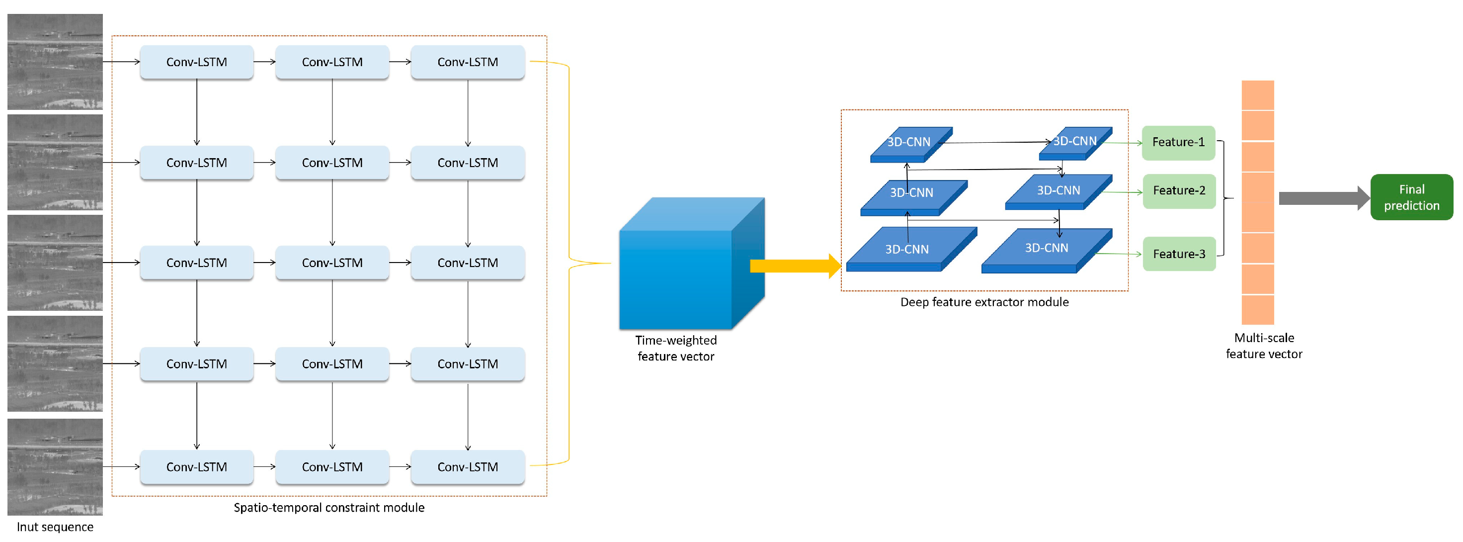
The full detection model is exhibited in Figure 5. It consists of two parts: a learning spatio-temporal constraint module (STM) and an extracting deep spatial features module (DFM). The STM is trained for learning the spatio-temporal constraints of multiple frames. The DFM is treated as a feature pyramid structure for learning the characteristics of different spatial dimensions between the target and the background. The input of the model is multiple frames, and the output is the prediction of the frames.

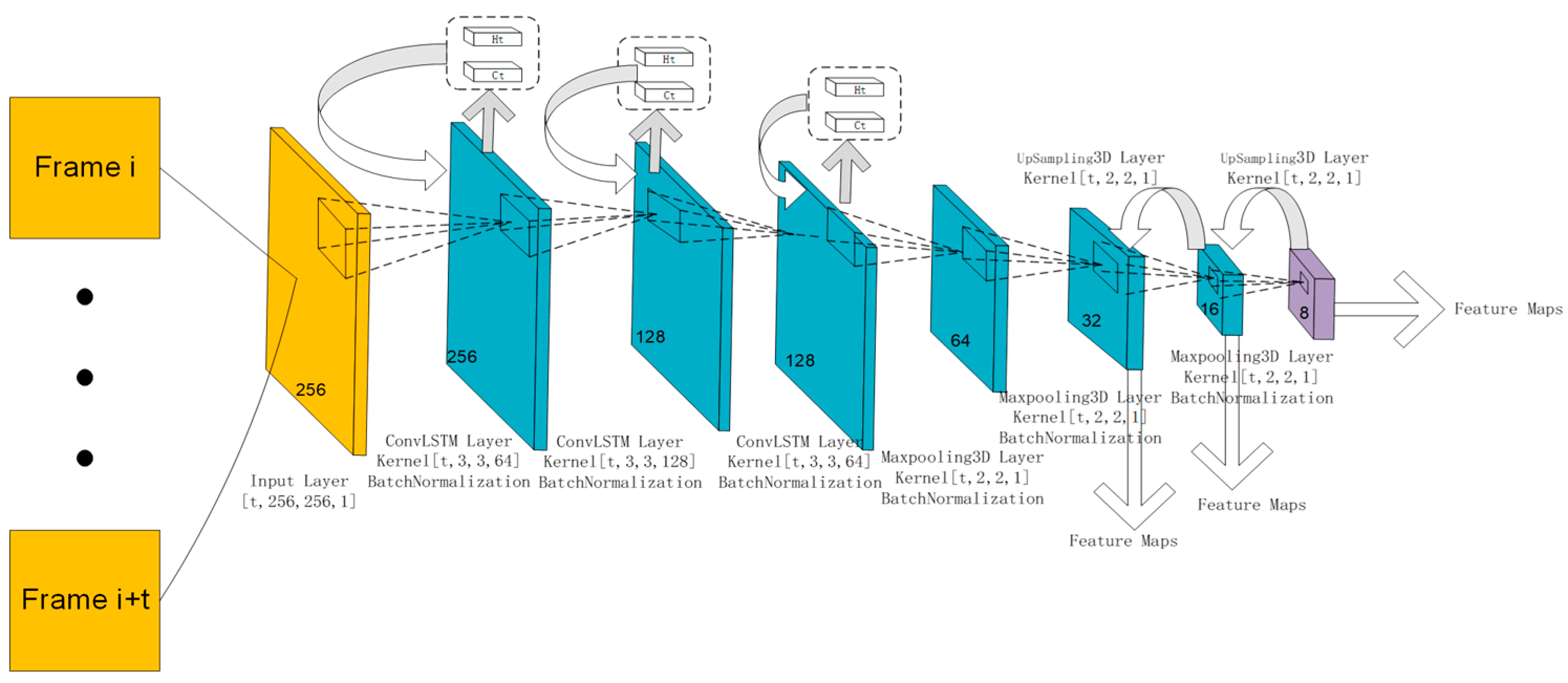
Specific layer designs are shown in Figure 6. The input layer has four parameters, which are input sequence length t, image resolution, and the number of channels. Given that infrared images are normally dominated by grayscale, we used a single channel as the network input. Then, there are three Conv-LSTM layers. The convolutional kernel sizes are [t, 3, 3, 64], [t, 3, 3, 128], and [t, 3, 3, 64]. The design of the dimension and the channel comply with universal design rules and real experimental effects. To preserve feature maps in the temporal dimension, 3D convolutional kernels are used for the next max pooling operation. The parameter meaning is kept consistent with the preorder layer. Next, the same scale layers would be directly concatenated after up-sampling operations. The output of the network has three patterns: 8, 16, and 32 scales. The choice of scales mainly takes into account the size of the target. Before the calculation of the loss function, we integrated multi-scale feature maps for ease of calculation, which makes use of the list in Python. Notice that we placed batch normalization layers after each feature extraction layer mainly to accelerate the convergence of the model. The batch normalization layers could remove the correlation between features and make all features possess the same mean and variance [25].

2.1.3. Learning Spatio-Temporal Constraint Module

Traditional multiple-frame-based methods usually use fixed parameters to estimate the motion model. However, in real-world scenarios, the velocity and the movement direction of the target are uncertain. In response, the methods often need costs that are too high and that involve more calculations relative to real-time applications [26,27]. Inspired by the success of the vision NLP (Nature Language Processing) model, we adopt Conv-LSTM’s structure to learn the spatio-temporal constraints of the target. Benefitting from timing and modeling capabilities, the Conv-LSTM structure could automatically analyze the motion model of the original data.

The basic LSTM structure is proposed for long-term predictions by its input gate, forget gate, and output gate. The workflow of the Conv-LSTM in this paper resembles a variable weighting machine. For the image sequence, the background and the target are fed into the input gate identically. Then, the forget gate decides the correlation between the current pixels and the previous pixels. Compared with the relatively stationary background, the trajectory features of the moving target are stored and transmitted to the next frame. The structure of the Conv-LSTM [28] is similar to the original LSTM structure except that the input and output are all 3D tensors, which represent the length of the sequence and the dimension of the single frame, respectively. In addition, the multiply operation is replaced with the convolution of the images. Thereupon, the memory cell is not only a sequence accumulator but a spatial feature extractor. The structure of STM is shown in Figure 7.

Multiple Conv-LSTM layers could improve the memory ability of the network [28]. Considering the size of the target and the resolution of the dataset images, we chose 3 layers to learn the sequence’s motion feature. C_i,j implies the cell status of the timeline. H_i,j is the output of the single cell. i denotes the network layer, and j denotes the specific unit. Pool is the pooling layer. It is employed to refine the learning result. The output of the STM is the time-weighted feature layer, which is displayed by the pink square.

2.1.4. Extracting Deep Spatial Features Module

After being processed by the spatio-temporal constraint module, the input frames are weighed by the temporal relationship, as shown in Figure 8. The left shows the processing of the single-frame image. The local contrasts of the target and the background are very similar. It is indistinguishable in the spatial dimension alone. The right indicates that the model with spatio-temporal constraints has superior results. For the single-frame method based on the local gradient, segmenting the target effectively is difficult when the target is very small and lacks texture features.

The feature pyramid network (FPN) module has been applied extensively to universal target detection in recent studies. It extracts multi-scale features for fusion, thereby improving detection accuracy. Motivated by that, the DFM is joined behind the spatio-temporal module. Statistically, the size of the target may change between 2 × 2 and 7 × 7, and the general convolutional kernel and pooling operation might lose information. Hence, we chose feature maps with areas of 8, 16, and 32 scales. The fusion process is performed by up-sampling and down-sampling between different scales.

Notice that we used 3D-CNN instead of the commonly used 2D-CNN. Since the 3D structure contains a temporal dimension compared to the 2D convolution, it is more appropriate for multiple-frame detection algorithms. Figure 9 shows a group of feature maps at different scales.

The loss function in this paper comprised two parts: coordinate regression loss and confidence loss. Equation (1) is the coordinate regression loss referenced in CIoU [29] (Complete IoU Loss; IoU: Intersection over Union). It evaluates the area intersection ratio, the distance relationship, and the aspect ratio’s similarity between predicted and true coordinates. Equation (4) is the confidence loss [30], which is drawn upon to match with the former. It estimates the beingness of an object and picks out the best matching coordinate. Equation (6) indicates that the two component losses are linearly integrated during training.

$$L_{CIoU\left(bo{x}_{pre},bo{x}_{gt}\right)}=1-IoU\left(bo{x}_{pre},bo{x}_{gt}\right)+\frac{{\rho }^2\left(bo{x}_{pre},bo{x}_{gt}\right)}{c^2}+\alpha \upsilon$$

(1)

$$\upsilon =\frac{4}{{\pi }^2}(\mathit{arctan}\frac{w^{gt}}{h^{gt}}-\mathit{arctan}\frac{w}{h}{)}^2$$

(2)

$$\alpha =\frac{\upsilon }{(1-IoU)+\upsilon }$$

(3)

$$L_{con}=\stackrel{\wedge }{y}\mathit{log}(y)+(1-\stackrel{\wedge }{y})\mathit{log}(1-y)$$

(4)

$$y=P\ast IoU\left(bo{x}_{pre},bo{x}_{gt}\right)$$

(5)

$$loss={\displaystyle \sum }_i{\displaystyle \sum }_j{L}_i^j{}_{CIoU\left(bo{x}_{pre},bo{x}_{gt}\right)}+{\displaystyle \sum }_i{\displaystyle \sum }_j{L}_i^j{}_{Con}$$

(6)

In Equation (1), box_pre and box_gt, respectively, mean the network prediction and true coordinates. Part 1 − IoU (box_pre, box_gt) evaluates the overlapping area of the network prediction and true coordinates. ρ (box_pre, box_gt) computes the Euclidean distance. C represents the diagonal length of the minimum bounding box, which encircles box_pre and box_gt. The second part computes the distance of center point between the prediction and the true label. υ compares the consistency of the aspect ratio. w is the width of the prediction box, and h is the height. Accordingly, w^gt and h^gt are the parameters of the true box. α is a positive coefficient computed by υ and IoU. The third part is used to control the convergence of the width and height as quickly as possible. Equation (4) is the confidence. It is evaluated by Equation (5), where p denotes the probability of the object. P = 0 means no target in the box, and conversely, p = 1 means there exists targets.

In the training phase, the convolution operation in the network obeys the principle of parameter sharing. This reduces the number of parameters and achieves a more concise operation.

2.2. Inference Phase

State-Aware Module

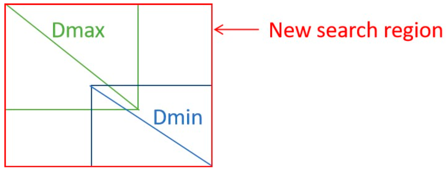
Infrared targets in long-range distances always occupy a few pixels of the entire image and represent only little semantic information [31]. The methods used early to improve the detection rate generally include pixel-by-pixel methods [32,33]. This causes many redundant calculations. A substantial amount of computation results are insignificant. This tends to cause online stability detection failures [34]. In this paper, we proposed an innovation called a state-aware module (STAM) to tackle the dilemma. It is a variable interval search strategy. The STAM records the historical diagonal of the prediction box, which is denoted as (D_max, D_min). D_max = D_min = D is initialized with the diagonal of the image to be detected. (D_max, D_min) is updated after the completion of k consecutive frames detection. k is set up as 5 due to the speed used in this paper. Provided that (D_max, D_min) is updated, the next search region will be replaced from the global image to the local neighborhood. The region is defined as the rectangular box enclosing (D_max, D_min), as shown in Figure 10. Such a pattern of local searches can greatly reduce the parameters of network computation and speed up the real-time applicability of the algorithm.

Next, consider the interruption case. If the target is temporarily lost from the local area due to sudden fast movements or frame loss, (D_max, D_min) is reinitialized to the global search. However, if the obstruction occurs, global research would also be futile. Inspired by the Simple Online and Realtime Tracking with a Deep Association Metric (Deep SORT) [35], we introduce the Kalman Filter (KF) to solve this situation, as shown in Figure 11. KF utilizes the motion correlation of the object to estimate the position [36,37]. When the obstruction is over, the model can quickly switch to the local search. As the parameters passing into the KF are only the positions, the computation does not consume many resources.

The stability of the algorithm matters for real applications, but uncontrollable factors (such as occlusion and frame loss) are unavoidable. STAM can improve the resilience and robustness of the model to solve unexpected events.

3. Results and Discussion

In this subsection, the experimental results are elaborated on with respect to three parts: (1) introduction to datasets; (2) evaluation metrics; (3) performance comparison and discussion.

3.1. Introduction to Datasets

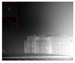
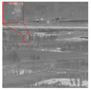
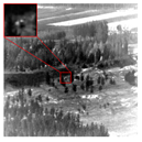
The experiments are executed on public [38] and author-collected infrared UAVs datasets. The resolutions of the image are, respectively, 256 × 256 and 640 × 512. The detection distance is from 1000 m to 5000 m. We adopt the SNR to describe the quantity of the image, as shown in Equation (7). The SNR of the datasets varies from 1 to 7.

Table 1. Details about 6 representative datasets.

	Image Examples	Resolution	SNR	Frame Number	Scene Description
Dataset 1		640 × 512	1.06	1500	Sky background
Dataset 2		640 × 512	1.75	1000	Asphalt road and grassy background
Dataset 3		640 × 512	2.09	4000	Buildings Background
Dataset 4		256 × 256	5.45	3000	Ground background
Dataset 5		256 × 256	3.42	750	Field background
Dataset 6		256 × 256	2.20	500	Vegetation background

. displays six representative datasets, including backgrounds of sky, sky-ground, and ground. The red box outlines the target of the raw image. Datasets 1–3 are from the author, and datasets 4–6 are from the publication:

$$SNR=\frac{{\mu }_t}{{\sigma }_b{}_{}}$$

(7)

where μ_t denotes the gray average of the target. σ_b denotes the standard deviation of the periphery. We take the target as the center and select the surrounding 10 × 10 area as the calculation field.

3.2. Evaluation Metrics

To conduct a comprehensive evaluation, three widely used metrics are adopted. The Intersection over Union (IoU) is used to conduct a pixel-level evaluation. Detection Rate (DR) and False Alarm (FA) are computed to describe the location ability of the method.

Intersection over Union (IoU): The IoU computes the ratio of the intersection (A_Inter) and union area (A_All) between the predictions and labels. It evaluates the spatial detection performance of the model, which is defined as follows.

$$IoU=\frac{A_{Inter}}{A_{All}}$$

(8)

Detection Rate (DR): DR computes the ratio of the correctly predicted target (T_Correct) number over all target numbers (T_All), and it is defined as follows.

$$DR=\frac{T_{Correct}}{T_{All}}$$

(9)

when the prediction is higher than the IoU threshold, we consider it as a correct prediction. The IoU threshold is set as 0.5 in this paper.

False-Alarm Rate (FA): FA evaluates the false alarm rate of the detection. It computes the ratio of false pixels detected (P_False) over total pixels (P_All) in the image, and it is defined as follows:

$$FA=\frac{P_{False}}{P_{All}}$$

(10)

3.3. Performance Comparison and Discussion

The proposed model uses Python3.8 and TensorFlow 2.4.0. All the experiments were conducted on an Ubuntu 20.04.4 LTS system with NVIDIA GeForce RTX 3090 GPU, 24 GB video memory. The parameter settings of the model are shown in

Table 2. The parameters of the entire model.

Layer	Parameter
conv-lstm-2D_0 (ConvLSTM)	9856
batch_normalization_0 (BatchNormalization)	64
conv-lstm-2D_1 (ConvLSTM)	55,424
batch_normalization_1 (BatchNormalization)	128
conv-lstm-2D_2(ConvLSTM)	27,712
batch_normalization_2 (BatchNormalization)	64
conv3d_0 (Conv3D)	6928
batch_normalization_3 (BatchNormalization)	64
conv3d_1 (Conv3D)	3464
batch_normalization_4 (BatchNormalization)	32
conv3d_2 (Conv3D)	3472
batch_normalization_5 (BatchNormalization)	64
up_sampling3d_0 (UpSampling3D)	0
up_sampling3d_1 (UpSampling3D)	0
concatenate (Concatenate)	0
concatenate (Concatenate)	0
Total params	107,272
Trainable params	107,064
Non-trainable params	208

. All the input frames of various sizes were normalized to 256 × 256. The validation and training sets were split in the ratio of 1:9. The batch size was set to 8, and the learning rate was initialized with 1 × 10⁻⁴. The epoch was initialized as 100.

3.3.1. Comparison to State-of-the-Art Methods

A sufficient number of experiments were conducted to investigate the performance of the proposed method and the current best models in this subsection. To comprehensively reflect their effectiveness, we compare the proposed model to six state-of-the-art (SOTA) methods, including recurrent YOLO (ROLO) [39], infrared small target detection with GAN (IRSTD-GAN, GAN: Generative Adversarial Network) [40], dynamic programming algorithm (DP) [11], time variance filter algorithm (TVF) [10], weighted strengthened local contrast measure (WSLCM) [41], and the multi-scale Laplacian of Gaussian (MCLoG) [42]. ROLO and IRSTD-GAN are representatives of CNN-based methods. DP and TVF are representatives of multiple-frame methods. WSLCM and MCLoG are classical single-frame detection methods.

For the sake of fairness, CNN-based methods are retrained on our datasets. Moreover, for traditional methods, we follow the parameters of the original paper for our experiments. The partially set parameters are shown in

Table 3. Partially set parameters for SOTA methods.

Method	Parameter Setting
TVF	T = 16, S_Z = 8
DP	T = 8
WSLCM	K = 9, λ = 0.8
MCLoG	K = 4
Proposed Method	T = 5

. For the TVF, the time domain window size T and the iteration step_size are, respectively, T = 16 and S_Z = 8. For the DP, the number of frames in batch processing is T = 8. For the WSLCM, the coefficient of the Gaussian filter is set to K = 9, and the factor of the threshold operation is set to λ = 0.8. For the MCLoG, the number of scales is set to K = 4. Considering that the moving speed of the target in our dataset is no more than five pixels, the input frame length of the proposed method in the experiment is supposed to be T = 5.

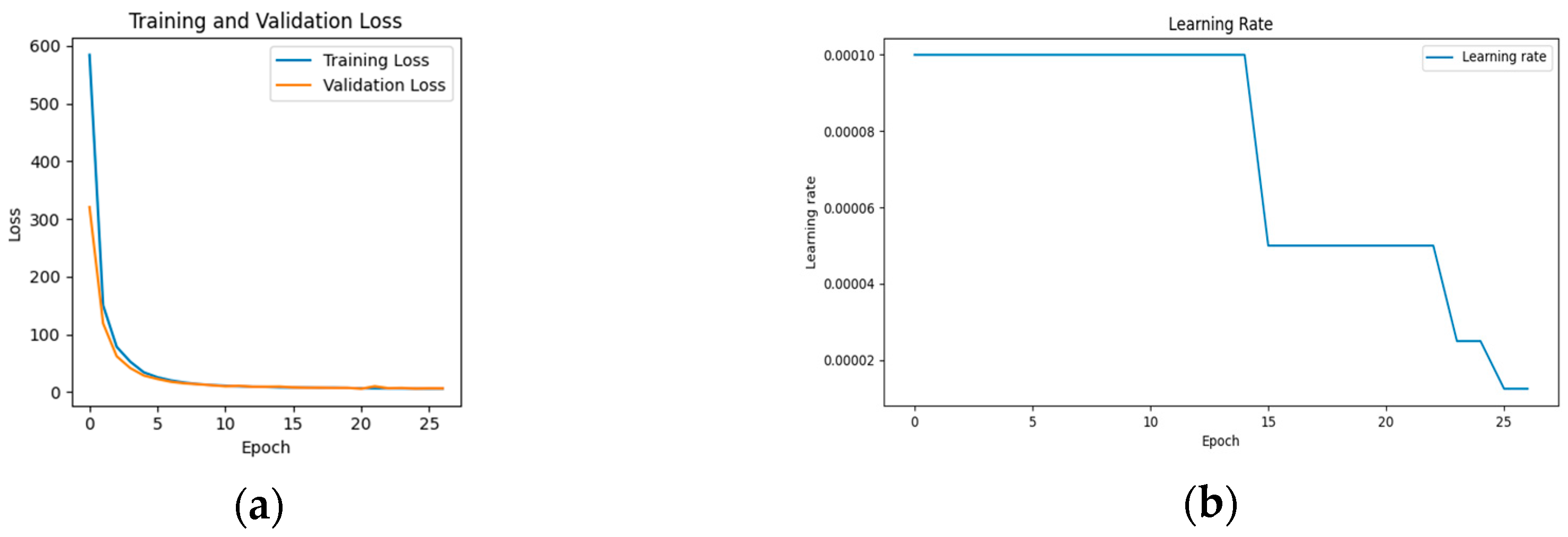
Figure 12 shows the convergence of our model. Figure 12a plots the training error curve and the validation variation tendency. It can be seen that the loss value decreases considerably at the beginning of the training phase, indicating that the learning rate is appropriate and the gradient descent process is performed. The loss curve tends to smooth out after a certain stage of learning, and the network achieves convergence. Figure 12b visualizes the evolution of the learning rate. As shown in the subplot, the learning rate decreases normally during the training phase and stabilizes after 25 epochs.

The quantity of the discussed methods is subsequently assessed by using DR and FA.

Table 4. We compute IoU, DR, and FA on public dataset and author-collected dataset with different SOTA methods. For IoU and DR, a higher value means better results. However, a smaller value of FA means that the approach works better. The best results are shown in bold.

Method	Author-Collected Dataset			Public Dataset
	IoU (×10−2)	DR (×10−2)	FA (×10−2)	IoU (×10−2)	DR (×10−2)	FA (×10−2)
WSLCM [32]	2.81	32.97	19.40	3.78	45.96	13.76
MCLoG [33]	9.78	45.35	26.78	19.78	53.16	7.04
DP [11]	60.75	66.97	7.93	73.65	77.94	17.9
TVF [10]	59.54	61.81	17.18	65.32	75.16	8.49
ROLO [30]	50.32	73.97	0.732	65.08	84.57	0.45
IRSTD-GAN [40]	45.68	76.31	3.45	75.32	86.16	1.38
Proposed	86.99	95.87	0.10	88.65	97.96	0.02

shows the quantitative results. Traditional single-frame methods (WSLCM and MCLoG) have a positive detection rate as well as a high false alarm rate. This is particularly evident in self-made datasets with more isolated noise. They fail to distinguish isolated points caused by sensor inhomogeneities because these two methods are based on gradient differences between the target and the background, whereas the pseudo-target shares this property.

The multiple-frame methods (DP and TVF) exploit the temporal association of the target, which partly alleviates the false alarm rate. However, when the background becomes complex and variable, the algorithm commences to become less effective. The temporal model with fixed parameters is not adaptable to prolonged detection.

ROLO and the IRSTD-GAN acquire acceptable results. The false alarm rate of CNN-based methods is relatively substantial because they are trained via datasets to extract more stable features. However, ROLO needs to pretrain the detector, and then, the LSTM solely learns the temporal features of the spatial results. It is inevitable that the model needs more trajectory data to train. In our small dataset, it performs badly. The IRSTD-GAN is a single-frame method, which works well for static targets, but the results of the moving targets are fair.

One can see that the proposed method reaches the trade-off between detection accuracy and false alarm. This is attributed to the fact that the Conv-LSTM structure learns the spatio-temporal constraint of the moving target and the deep feature extractor based on 3D-CNN and fuses multi-scale local features between the target and the background.

The proposed method yields better performances than the baseline algorithms in terms of both the detection rate and false alarm rate. The CNN-based methods are generally better than the traditional methods. This benefits from the flexible feature learning. However, the ROLO and IRSTD-GAN require more datasets, limiting their performance. The multiple-frame-based methods suffer less from the influence of pseudo-targets and achieve lower false alarm than the single-frame method. The traditional methods depend heavily on fixed parameter kernels. They sacrificed false alarm rates to ensure detection rates. Our method is more robust to moving targets and complex environments.

3.3.2. Qualitative Evaluation

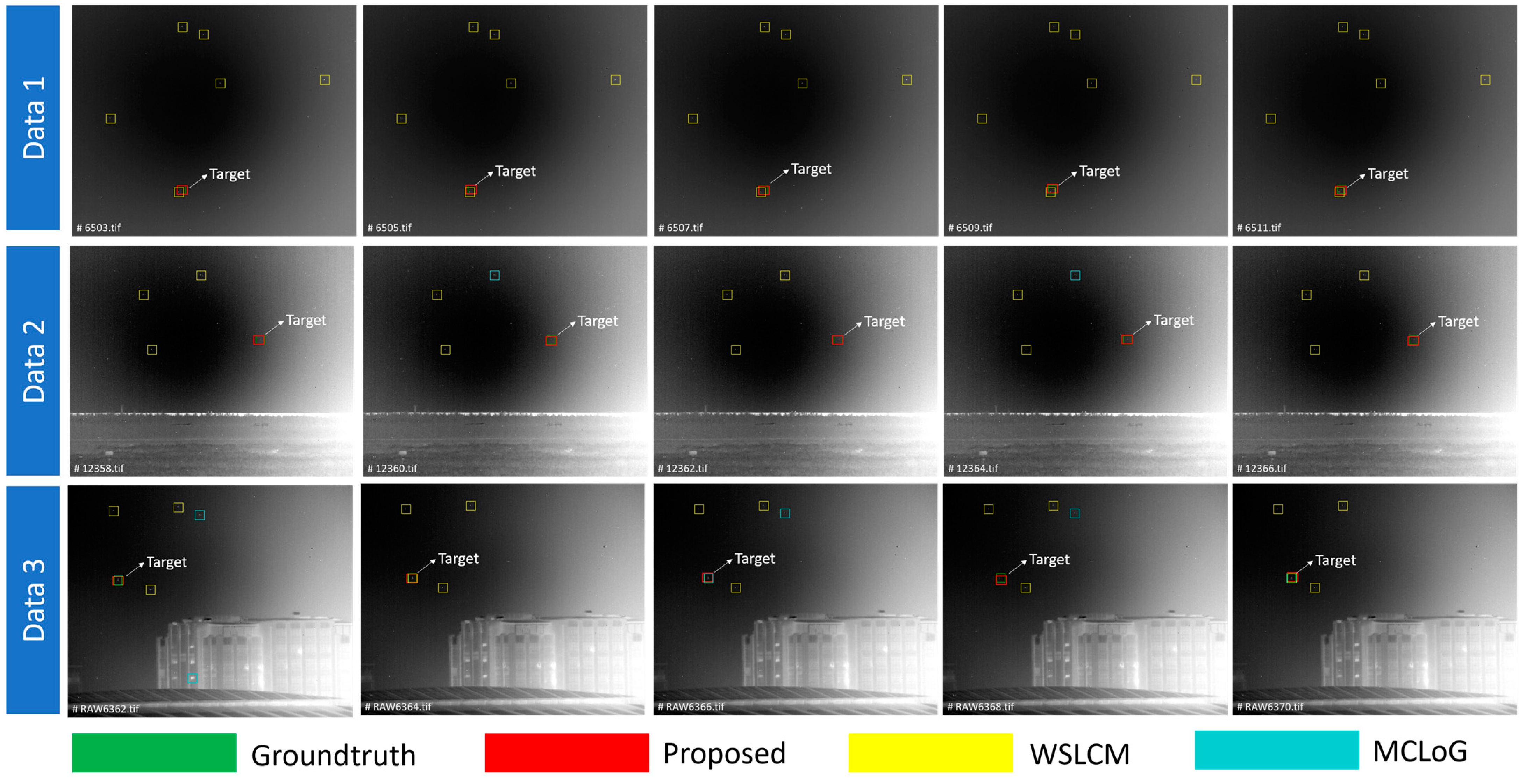
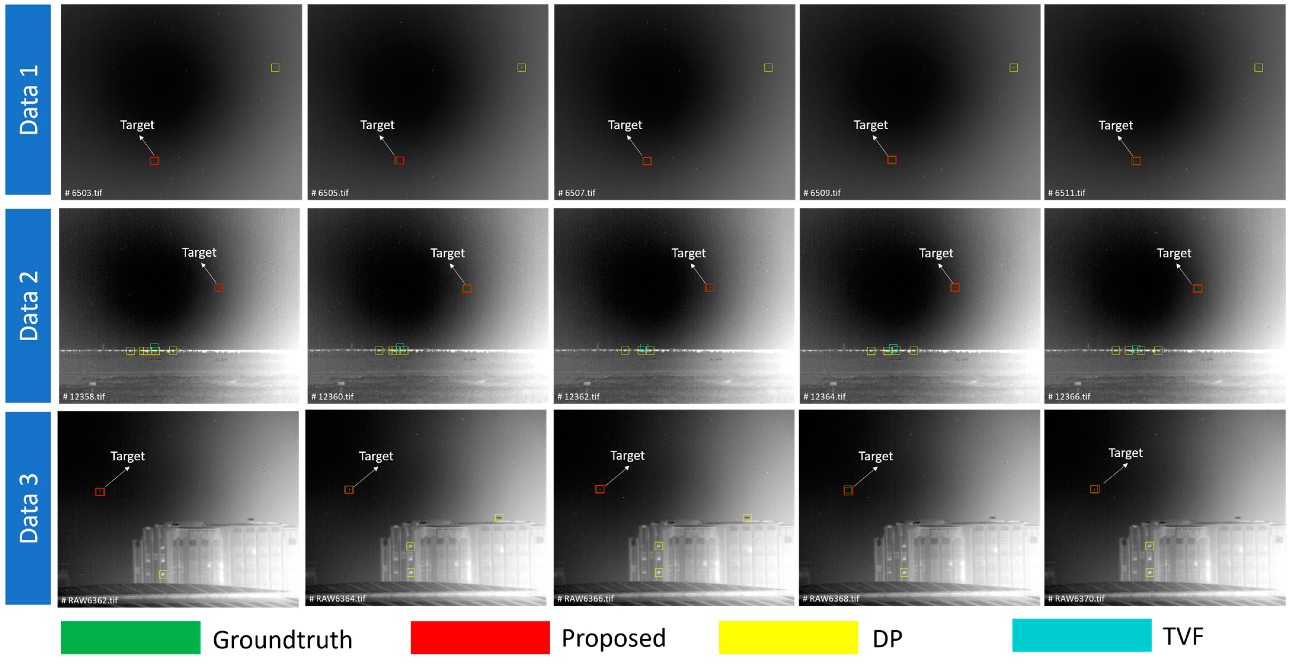
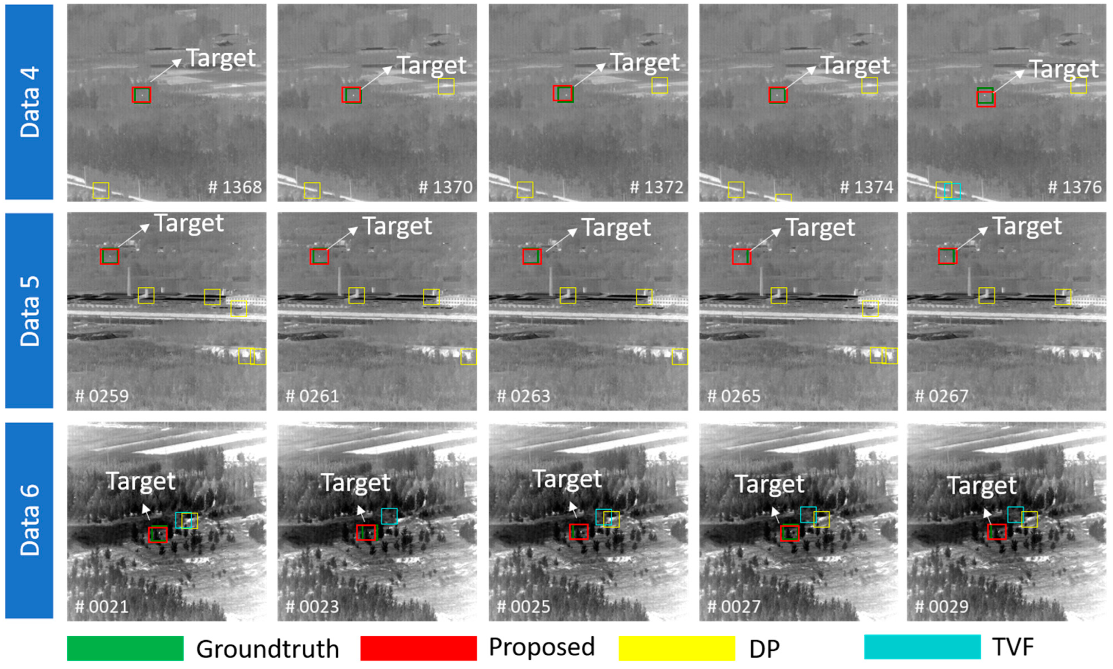
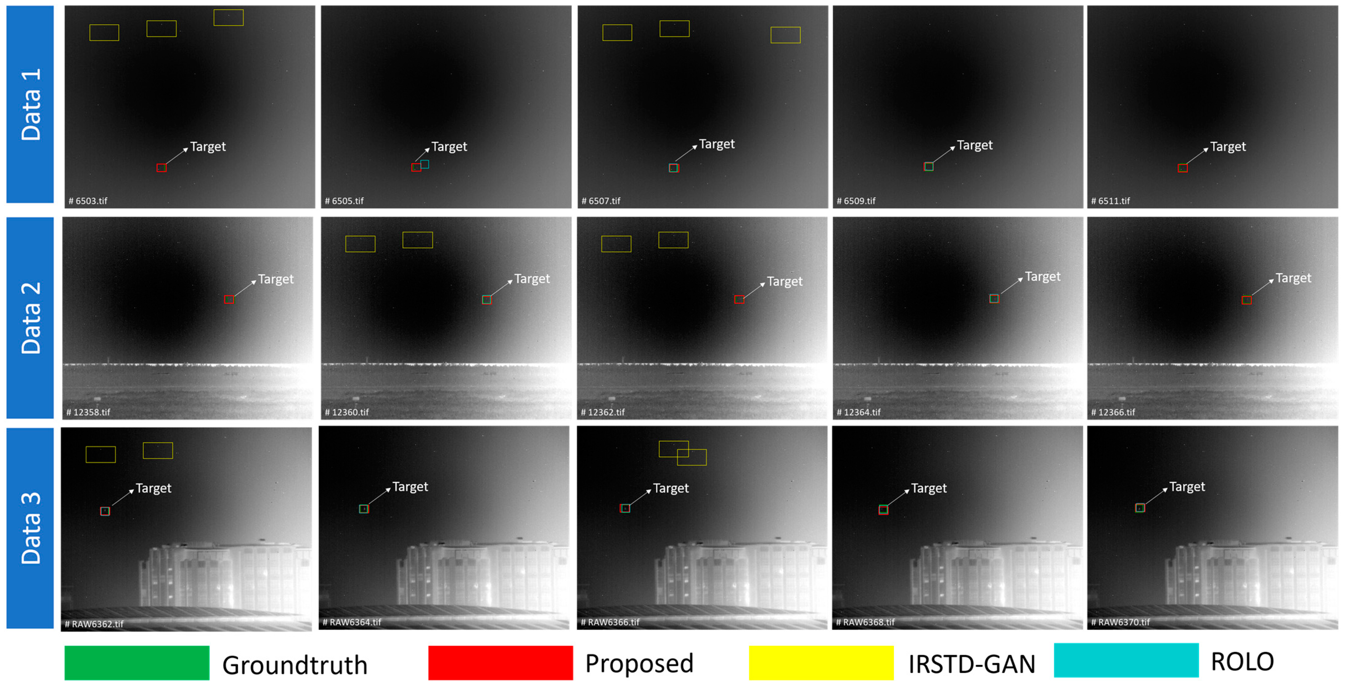
Figure 13, Figure 14, Figure 15, Figure 16, Figure 17 and Figure 18 visualize the qualitative comparison of the proposed model and other SOTA methods. It can be seen that the proposed method achieves an efficient and robust detection in a diversity of backgrounds.

Figure 13 and Figure 14 show detection results between the proposed method and traditional single-frame-based methods. In Dataset 1–Dataset 3, the isolated noise points caused by the nonuniformity of the infrared sensor exist in each frame. When the target size turns a few pixels, the local contrast is similar to the isolated noise points. It is difficult to pick out the true target for the traditional methods. Instead, the neural network extracts more stable features of the object. For Dataset 4–Dataset 6, the background becomes complex. Swaying trees and high glossy tarmac roads are present in the frame. The traditional single-frame-based methods are easily confused by them. The false alarm rate is quite high. However, our method still achieves excellent performance.

Figure 15 and Figure 16 display the comparison between our method and traditional multiple-frame-based methods. Obviously, compared to single-frame methods, temporal cues of the consecutive frames improve the performance. It helps avoid most static pseudo-targets. However, the fixed parameter model cannot adapt to the random motion of the target. The detection rate, therefore, is not very satisfactory. For the proposed model, the estimation of the spatio-temporal constraint belongs to a flexible learning procedure. The experimental results show that it could make a more accurate prediction of the moving target.

Figure 17 and Figure 18 plot the detection of CNN-based methods. Overall, they yielded positive results. Public datasets with a relatively large number of training datasets have better results, especially for ROLO, which requires more motion information. Different from most CNN-based variants for infrared small target detection, our method adds a state-aware module, which helps conquer random issues, including fast motion, frame lost, and occlusion. The detection results indicate that this is valid and helps in real-time applications.

3.3.3. Ablation Study

The ablation study is applied to analyze the contributions of each component in the model. We divide the entire model into three sub-modules: spatio-temporal module (STM), deep feature module (DFM), and state-aware module (SATM). The first combination is the single STM, which only uses Conv-LSTM cells and flattens the final vector to detect targets. The second combination is a single DFM. The third combination is STM + DFM without a dynamic search strategy. The fourth combination is STM + SATM, and the last combination is DFM + SATM.

The ablation experiments are implemented on unified datasets. The results are shown in

Table 5. Ablation studies on the components of our method. The self-made dataset is taken as a sample.

Submodule			Evaluation Metric
STM	DFM	STAM	IoU (×10−2)	DR (×10−2)	FA (×10−2)
√			43.60	60.15	4.63
	√		56.27	77.33	7.87
√	√		85.69	90.28	1.03
√		√	48.73	69.45	2.32
	√	√	55.69	78.64	1.11
√	√	√	86.99	95.87	0.10

and

Table 6. Ablation studies on components of our method. The public dataset is taken as a sample.

Submodule			Evaluation Metric
Spatio-Temporal Module	Multiscale Feature Module	State-Aware Module	IoU (×10−2)	DR (×10−2)	FA (×10−2)
√			50.92	75.43	7.35
	√		48.37	80.79	4.36
√	√		83.68	92.86	0.51
√		√	51.78	83.59	1.36
	√	√	50.36	81.54	1.29
√	√	√	88.65	97.96	0.02

. One can see that multiple-frame detection can improve the accuracy of the algorithm compared to the spatial feature approach alone. It, respectively, improves the detection rate by 12.95% and 17.43% in self-made datasets and public datasets. This can be attributed to the joint detection of the spatio-temporal feature. The addition of the state-aware module, respectively, improves the accuracy by 5.59% and 5.10% in self-made datasets and public datasets. Moreover, it, respectively, reduces false alarms by 1.01% and 1.27%. These illustrate the effectiveness of the intervention module in the inference phase. Overall, the proposed method obtains satisfactory results in terms of IoU, detection rates, and false alarm rates.

4. Conclusions

In this paper, a learning motion constraint-model-based spatio-temporal network is proposed for detecting infrared dim targets. It consists of three submodules: the spatio-temporal feature extractor (STM), deep feature extractor (DFM), and state-aware module (STAM). The STM is trained to weigh the image sequence from the temporal perspective. Subsequently, the DFM is applied to broaden the receptive field, and it fuses multiscale features between the target and the background. In the inference, with the purpose of improving the robustness and practicality, the STAM is used to solve the redundancy calculation, background occlusion, and frame loss encountered. Experimental results reveal that the method obtains higher accuracies and lower false alarms than the baseline algorithms, even over a low SNR.

This method would hopefully be applied to IRST for anti-UAV remote monitoring and early warnings. Divergent from existing single-frame-based deep learning methods, the proposed method introduces recurrent networks to learn the temporal feature of moving targets. The experiments demonstrate the potential of multi-frame-based neural networks and emphasize the importance of the joint detection of spatial-temporal information. However, the LSTM cell inevitably needs magnanimous training datasets to learn the motion feature, which reduces its usefulness in particular circumstances. In addition, the proposed method still involves manual hyperparameters, such as the length of input frames determined by the motion speed. The manual parameter also limits applications. In the future, self-supervised training without labels will be discussed for improving the network’s training and the intelligence of the method.

References

1. Hu, Y.; Xiao, M.; Li, S.; Yang, Y. Aerial infrared target tracking based on a Siamese network and traditional features. Infrared Phys. Technol. 2020, 111, 103505. [Google Scholar] [CrossRef]
2. Liu, R.; Wang, D.; Jia, P.; Sun, H. An Omnidirectional Morphological Method for Aerial Point Target Detection Based on Infrared Dual-Band Model. Remote Sens. 2018, 10, 1054. [Google Scholar] [CrossRef] [Green Version]
3. Guan, X.; Zhang, L.; Huang, S.; Peng, Z. Infrared Small Target Detection via Non-Convex Tensor Rank Surrogate Joint Local Contrast Energy. Remote Sens. 2020, 12, 1520. [Google Scholar] [CrossRef]
4. Zhang, Y.; Zheng, L.; Zhang, Y. Small Infrared Target Detection via a Mexican-Hat Distribution. Appl. Sci. 2019, 9, 5570. [Google Scholar] [CrossRef] [Green Version]
5. Rao, J.; Mu, J.; Li, F.; Liu, S. Infrared Small Target Detection Based on Weighted Local Coefficient of Variation Measure. Sensors 2022, 22, 3462. [Google Scholar] [CrossRef]
6. Pan, S.D.; Zhang, S.; Zhao, M.; An, B.W. Infrared Small Target Detection Based on Double-layer Local Contrast Measure. Acta Photonica Sin. 2020, 49, 110003. [Google Scholar]
7. Wu, L.; Ma, Y.; Fan, F.; Wu, M.; Huang, J. A Double-Neighborhood Gradient Method for Infrared Small Target Detection. IEEE Geosci. Remote Sens. Lett. 2020, 18, 1476–1480. [Google Scholar] [CrossRef]
8. Sun, Y.; Yang, J.; Li, M.; An, W. Infrared Small-Faint Target Detection Using Non-i.i.d. Mixture of Gaussians and Flux Density. Remote Sens. 2019, 11, 2831. [Google Scholar] [CrossRef] [Green Version]
9. Kwan, C.; Budavari, B. Enhancing Small Moving Target Detection Performance in Low-Quality and Long-Range Infrared Videos Using Optical Flow Techniques. Remote Sens. 2020, 12, 4024. [Google Scholar] [CrossRef]
10. Lv, P.-Y.; Lin, C.-Q.; Sun, S.-L. Dim small moving target detection and tracking method based on spatial-temporal joint processing model. Infrared Phys. Technol. 2019, 102, 102973. [Google Scholar] [CrossRef]
11. Yi, W.; Fang, Z.; Li, W.; Hoseinnezhad, R.; Kong, L. Multi-Frame Track-Before-Detect Algorithm for Maneuvering Target Tracking. IEEE Trans. Veh. Technol. 2020, 69, 4104–4118. [Google Scholar] [CrossRef]
12. Girshick, R. Fast R-CNN. arXiv 2015, arXiv:1504.08083. Available online: https://ui.adsabs.harvard.edu/abs/2015arXiv150408083G (accessed on 1 April 2015).
13. Redmon, J.; Farhadi, V.; Recognition, P. YOLO9000: Better, Faster, Stronger. In Proceedings of the IEEE Conference on Computer Vision and Pattern Recognition, Honolulu, HI, USA, 21–26 July 2017; pp. 6517–6525. [Google Scholar]
14. Redmon, J.; Farhadi, A.J.A. YOLOv3: An Incremental Improvement. arXiv 2018, arXiv:1804.02767. [Google Scholar]
15. Liu, W.; Anguelov, D.; Erhan, D.; Szegedy, C.; Reed, S.; Fu, C.; Berg, A.C. SSD: Single Shot MultiBox Detector. In Lecture Notes in Computer Science, Proceedings of the omputer Vision–ECCV, Amsterdam, The Netherlands, 11–14 October 2016; Springer: Cham, Switzerland, 2016. [Google Scholar]
16. Lin, T.-Y.; Goyal, P.; Girshick, R.B.; He, K.; Dollár, P.; Intelligence, M. Focal Loss for Dense Object Detection. IEEE Int. Conf. Comput. Vis. 2020, 42, 318–327. [Google Scholar] [CrossRef] [PubMed] [Green Version]
17. Ryu, J.; Kim, S. Heterogeneous Gray-Temperature Fusion-Based Deep Learning Architecture for Far Infrared Small Target Detection. J. Sens. 2019, 2019, 4658068. [Google Scholar] [CrossRef] [Green Version]
18. Wang, H.; Li, H.; Zhou, H.; Chen, X. Low-altitude infrared small target detection based on fully convolutional regression network and graph matching. Infrared Phys. Technol. 2021, 115, 103738. [Google Scholar] [CrossRef]
19. Shi, M.; Wang, H. Infrared Dim and Small Target Detection Based on Denoising Autoencoder Network. Mob. Netw. Appl. 2019, 25, 1469–1483. [Google Scholar] [CrossRef]
20. Ju, M.; Luo, J.; Liu, G.; Luo, H. ISTDet: An efficient end-to-end neural network for infrared small target detection. Infrared Phys. Technol. 2021, 114, 103659. [Google Scholar] [CrossRef]
21. Miller, J.L.; Kim, S. Small infrared target detection by data-driven proposal and deep learning-based classification. In Proceedings of the Infrared Technology and Applications XLIV, Orlando, FL, USA, 23 May 2018; Volume 10624. [Google Scholar]
22. Liu, M.; Du, H.; Zhao, Y.; Dong, L.; Hui, M.; Wang, S.X. Image Small Target Detection based on Deep Learning with SNR Controlled Sample Generation. Curr. Trends Comput. Sci. Mech. Autom. 2017, 1, 211–220. [Google Scholar]
23. Yao, S.; Zhu, Q.; Zhang, T.; Cui, W.; Yan, P. Infrared Image Small-Target Detection Based on Improved FCOS and Spatio-Temporal Features. Electronics 2022, 11, 933. [Google Scholar] [CrossRef]
24. Wang, P.; Wang, H.; Li, X.; Zhang, L.; Di, R.; Lv, Z. Small Target Detection Algorithm Based on Transfer Learning and Deep Separable Network. J. Sens. 2021, 2021, 9006288. [Google Scholar] [CrossRef]
25. Ioffe, S.; Szegedy, C.J.A. Batch Normalization: Accelerating Deep Network Training by Reducing Internal Covariate Shift. arXiv 2015, arXiv:1502.03167. [Google Scholar]
26. Zhou, A.; Xie, W.; Pei, J. Background Modeling in the Fourier Domain for Maritime Infrared Target Detection. IEEE Trans. Circuits Syst. Video Technol. 2019, 30, 2634–2649. [Google Scholar] [CrossRef]
27. Wu, Y.; Wang, Y.; Liu, P.; Luo, H.; Cheng, B.; Sun, H. Infrared LSS-Target Detection Via Adaptive TCAIE-LGM Smoothing and Pixel-Based Background Subtraction. Photonic Sens. 2018, 9, 179–188. [Google Scholar] [CrossRef] [Green Version]
28. Kim, S.; Hong, S.; Joh, M.; Song, S.-k.J.A. DeepRain: ConvLSTM Network for Precipitation Prediction using Multichannel Radar Data. arXiv 2017, arXiv:1711.02316. [Google Scholar]
29. Zheng, Z.; Wang, P.; Liu, W.; Li, J.; Ye, R.; Ren, D. Distance-IoU Loss: Faster and Better Learning for Bounding Box Regression. In Proceedings of the AAAI Conference on Artificial Intelligence, New York, NY, USA, 7–12 February 2020; Volume 34, no. 07. pp. 12993–13000. [Google Scholar]
30. Bochkovskiy, A.; Wang, C.-Y.; Liao, H.-Y.M.J.A. YOLOv4: Optimal Speed and Accuracy of Object Detection. arXiv 2020, arXiv:2004.10934. [Google Scholar]
31. Eysa, R.; Hamdulla, A.; Automation, E. Issues on Infrared Dim Small Target Detection and Tracking. In Proceedings of the 2019 International Conference on Smart Grid and Electrical Automation (ICSGEA), Xiangtan, China, 10–11 August 2019; pp. 452–456. [Google Scholar]
32. Du, J.; Lu, H.; Zhang, L.; Hu, M.; Chen, S.; Deng, Y.; Shen, X.; Zhang, Y. A Spatial-Temporal Feature-Based Detection Framework for Infrared Dim Small Target. IEEE Trans. Geosci. Remote Sens. 2021, 60, 3000412. [Google Scholar] [CrossRef]
33. Yang, L.; Liu, S.; Zhao, Y. Deep-Learning Based Algorithm for Detecting Targets in Infrared Images. Appl. Sci. 2022, 12, 3322. [Google Scholar] [CrossRef]
34. Huang, B.; Chen, J.; Xu, T.; Wang, Y.; Jiang, S.; Wang, Y.; Wang, L.; Li, J. SiamSTA: Spatio-Temporal Attention based Siamese Tracker for Tracking UAVs. In Proceedings of the IEEE/CVF International Conference on Computer Vision, Virtual, 11–17 October 2021; pp. 1204–1212. [Google Scholar]
35. Wojke, N.; Bewley, A.; Paulus, D. Simple online and realtime tracking with a deep association metric. In Proceedings of the 2017 IEEE International Conference on Image Processing (ICIP), Beijing, China, 17–20 September 2017; pp. 3645–3649. [Google Scholar]
36. Xiao, S.; Ma, Y.; Fan, F.; Huang, J.; Wu, M. Tracking small targets in infrared image sequences under complex environmental conditions. Infrared Phys. Technol. 2020, 104, 103102. [Google Scholar] [CrossRef]
37. Zhu, Z.; Lou, K.; Ge, H.; Xu, Q.; Wu, X. Infrared target detection based on Gaussian model and Hungarian algorithm. Enterp. Inf. Syst. 2021, 16, 1573–1586. [Google Scholar] [CrossRef]
38. Hui, B.; Song, Z.; Fan, H.; Zhong, P.; Hu, W.; Zhang, X.; Ling, J. A dataset for infrared image dim-small aircraft target detection and tracking under ground / air background. Sci. Data Bank 2019, 5, 12. [Google Scholar]
39. Ning, G.; Zhang, Z.; Huang, C.; Ren, X.; Wang, H.; Cai, C.; He, Z. Spatially supervised recurrent convolutional neural networks for visual object tracking. In Proceedings of the 2017 IEEE International Symposium on Circuits and Systems (ISCAS), Baltimore, MD, USA, 28–31 May 2017; pp. 1–4. [Google Scholar]
40. Zhao, B.; Wang, C.; Fu, Q.; Han, Z. A Novel Pattern for Infrared Small Target Detection With Generative Adversarial Network. IEEE Trans. Geosci. Remote Sens. 2021, 59, 4481–4492. [Google Scholar] [CrossRef]
41. Han, J.; Moradi, S.; Faramarzi, I.; Zhang, H.; Zhao, Q.; Zhang, X.; Li, N. Infrared Small Target Detection Based on the Weighted Strengthened Local Contrast Measure. IEEE Geosci. Remote Sens. Lett. 2020, 18, 1670–1674. [Google Scholar] [CrossRef]
42. Moradi, S.; Moallem, P.; Sabahi, M.F. A false-alarm aware methodology to develop robust and efficient multi-scale infrared small target detection algorithm. Infrared Phys. Technol. 2018, 89, 387–397. [Google Scholar] [CrossRef]
Figure 1. The processing flow of the proposed method. It consists of two parts: training phase and inference phase. In the training phase, the spatio-temporal module (STM) firstly learns the motion constraint and the deep feature module (DFM) and secondly fuses the multiscale feature to achieve robust detections. In the inference phase, the state-aware module (STAM) is added to face emergencies during real-time detections.
Applsci 12 11519 g001
Figure 2. A single frame from the from the 5000 m distance video. The target is shown with a red rectangle. (a) The original infrared image; (b) the pixel distribution of the frame.
Applsci 12 11519 g002
Figure 3. An infrared image sequence from the same video. The target is shown with a red rectangle. (a) The original infrared image sequence; (b) optical flow estimation of the sequence. Pixel movement is rendered with colored blocks.
Applsci 12 11519 g003
Figure 4. The handing of the time stream. The index i, i − 1…, i − t in the square indicates the image sequence.
Applsci 12 11519 g004
Figure 5. Overview of the proposed model.
Applsci 12 11519 g005
Figure 6. Details of the network’s design. Parameter t is the length of the input sequence. Ht is the output of the single cell of Conv-LSTM, and Ct is the status of the single cell. The outputs are multiple scale feature maps.
Applsci 12 11519 g006
Figure 7. The workflow of STM in the proposed model. The STM has 3 Conv-LSTM layers followed by 1 pooling layer. It takes multiple frames as inputs, such as t frames. t is related to the targeted motion speed. We set t to 5 in this paper.
Applsci 12 11519 g007
Figure 8. A comparison of the single-frame-based and multiple-frame-based detection. It can be seen that multiple-frame-based detection offers more advantages.
Applsci 12 11519 g008
Figure 9. Multi-scale feature heat map: (a) 8 × 8 feature maps; (b) 16 × 16 feature maps; (c) 32 × 32 features. It can be seen that large scale feature maps are sensitive to small targets, while small scale feature maps are effective for large-sized objects such as backgrounds.
Applsci 12 11519 g009
Figure 10. A description of the search region.
Applsci 12 11519 g010
Figure 11. A description of the KF strategy in the STAM. KF utilizes the network prediction as input. The Kalman gain and covariance matrix are calculated to predict the possible location in the next frame by combining the current position. When uncertain obstructions occur, the KF prediction could ensure the continuity of detections without large fluctuations.
Applsci 12 11519 g011
Figure 12. A description of the convergence. The training loss and learning rate of our model tend to be stable after 25 epochs. (a) The training error curve and the validation variation tendency; (b) The learning rate curve of the training phase.
Applsci 12 11519 g012
Figure 13. Detection results between our method and traditional single-frame-based methods in self-made datasets. The target has been marked by texts, and the other prediction boxes are false alarms. Experimental results show that the proposed method has the highest coincidence with the ground truth.
Applsci 12 11519 g013
Figure 14. Detection results between our method and traditional single-frame-based methods in public datasets. The target has been marked by texts, and the other prediction boxes are false alarms. Experimental results show that the conventional single-frame algorithm has a high false alarm rate except for the proposed method.
Applsci 12 11519 g014
Figure 15. Detection results between our method and traditional multiple-frame-based methods in self-made datasets. The target has been marked by texts, and the other prediction boxes are false alarms. Experimental results show that only the method in this paper achieves continuous detections. The conventional multi-frame algorithm misidentifies the tarmac, the windows, and vegetation as targets.
Applsci 12 11519 g015
Figure 16. Detection results between our method and traditional multiple-frame-based methods in public datasets. The target has been marked by texts, and the other prediction boxes are false alarms. Experimental results show that only the method in this paper achieves continuous detections.
Applsci 12 11519 g016
Figure 17. Detection results between our method and CNN-based methods in self-made datasets. The target has been marked by texts, and the other prediction boxes are false alarms. Experimental results show that the proposed method has the highest coincidence with the ground truth. Experimental results show that the detection rate of other deep learning algorithms is obviously lower than the method in this paper.
Applsci 12 11519 g017
Figure 18. Detection results between our method and CNN-based methods in public datasets. The target has been marked by texts, and the other prediction boxes are false alarms. Experimental results show that the proposed method has the highest coincidence with the ground truth.
Applsci 12 11519 g018