Abstract
For the problem of classification and identification of defects in polyethylene (PE) gas pipelines, this paper firstly performs preliminary screening of the acquired images and acquisition efficiency of defective image acquisition was improved. Images of defective PE gas pipelines were pre-processed. Then, edge detection of the defective images was performed using the improved Sobel algorithm and an adaptive threshold segmentation method was applied to segment the defects in the pipeline images. Finally, the defect images were morphologically processed to obtain binary images. The obtained binary images were applied with VGG16 to complete the training of the defect classifier. The experimental findings show that in the TensorFlow API environment, the test set’s highest accuracy reached 97%, which can achieve the identification of defect types of underground PE gas transmission pipelines.
1. Introduction
In the past decades, polyethylene (PE) pipelines have been widely used in natural gas networks around the world because of their flexibility and corrosion resistance [1]. Therefore, the long-term performance of PE pipes and their materials is of great concern to date [2]. According to international natural gas pipeline accident statistics, natural gas pipeline defects are frequently caused by localized corrosion [3], operator mistakes, defective materials, and construction flaws [4]. As the use of pipelines for transporting hazardous substances becomes more popular worldwide, the possibility of major accidents caused by pipeline failures is gradually increasing [5]. For example, the explosion caused by a gas pipeline leak in a residential building in Slovakia in 2019, which killed at least seven people, reminds us that gas pipelines must be checked regularly [6]. There are many nondestructive inspection methods for gas pipelines in practice (e.g., ultrasonic-based sensors, laser-based systems, etc.), and compared to other inspection techniques commonly used for PE pipelines, due to their distinctive benefits of intuitiveness, accuracy and convenience, visual inspection techniques have been used extensively in a variety of fields [7]. Pipeline defect detection robots equipped with intra-visual inspection of image processing technology can directly collect, transmit and process images, reducing labor costs [8].
Traditionally, automatic classification of images is carried out using extracted image features, which are used to represent unclear information in the original pixel values. Convolutional neural networks (CNN) have taken the place of that approach in recent years [9]. Image pre-processing, which includes image de-noising [10], image enhancement [11], image segmentation [12], morphological operations [13], etc., is generally performed before image classification. Based on image pre-processing, Zhou et al. [14] investigated an improved spline local mean decomposition (ISLMD), proposed to be CNN-based and enabling noise reduction of images to locate pipe leakage locations. Ma et al. [15] proposed a sewer multi-defect detection system based on CNN-style GAN-SDM image pre-processing, and the proposed model’s average accuracy and macro F1 score were 95.64% and 0.955, respectively. Hosseinzadeh et al. [16] presented a small and simple probe design that was used to check small-bore pipes for defects. Hua et al. [17] developed a visual recognition-based pipeline fault detection algorithm. It is capable of both autonomous localization and pipeline fault detection.
Several frameworks based on the original CNN structure have been proposed to enhance target detection performance as a result of the advancement of CNN technology and classification, such as R-CNN [18], Fast R-CNN [19], SSD [20], YOLO series [21], etc. In this paper, a CNN-based classification framework for PE pipe defect detection is proposed, which can automatically extract the abstract features of defects for accurate classification of three defects, including cracks, fractures, and holes. In this paper, three different algorithms are applied to the existing framework and the confusion matrix is used to determine which model framework has the highest accuracy. The experimental results indicate that the highest accuracy of the test set in this paper reached 97% in the environment of TensorFlow API.
2. Image Pre-Processing
The pre-processing of pipe images does more than remove noise; it also enhances the contrast between the pipeline’s background and any pipeline defects, making it simpler to locate and categorize pipeline defects [22]. Figure 1 depicts the image pre-processing process used in this paper.

Figure 1.
Image pre-processing process.
2.1. Greyscale Processing for Pipeline Images
Grayscale is an important feature to characterize the brightness and darkness of an image. In recent years, on the basis of image grayscale differences and discontinuous changes, it has been used in target recognition, image segmentation, and machine vision technique [23]. Grayscale occupies less memory and enables faster computer operations compared to color images. The mean value method, maximum value method, and weighted average method are the three commonly used techniques for transforming color photos into grayscale.
Where the maximum value method is to directly take the value of the component with the largest value among the three components of a R,G,B Equation (1). Red (R), green (G) and blue (B) are the three color channels of color images.
The mean method is to take the mean of the values in the three components of R,G,B Equation (2).
The weighted average method is based on the sensitivity of the human eye for the R,G,B’s three colors, according to a certain weighted average, obtained in Equation (3).
where: I(u,v) denotes the gray value at coordinate, IR(u,v), IB(u,v) and IG(u,v) denote the luminance value of the pixel’s three color components, respectively.
The maximum value method (Figure 2B1–B3), the average value method (Figure 2C1–C3), and the weighted average method (Figure 2D1–D3) were used to grayscale process the three original defect images (Figure 2A1–A3) of cracks, fractures and holes, respectively. From Figure 2, it can be seen that the weighted average method produces the best results for the grayscale image, and the grayscale image has moderate brightness and does not cover the characteristics of the pipe defects. As a result, the image grayscale uses the weighted averaging method.
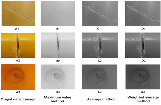
Figure 2.
Comparison of grayscale processing methods for pipe defect images.
2.2. Defect Image Acquisition
We compared and examined the continuously captured PE pipeline images and discovered that: 1. the percentage of pipeline defects in the entire PE gas pipeline network system is small; 2. there is a significant grayscale discrepancy between the defective and normal parts of the grayscale processed defective images; 3. after grayscale processing of any two adjacent PE pipeline images, there is a significant grayscale discrepancy between the normal PE pipeline images and the defective PE pipeline images in the same position, while the grayscale discrepancy between the two normal PE pipeline images is very small. Thus, in order to determine whether there are defects in the pipeline images, we propose a screening method for pipeline defects to improve the detection effectiveness [24].
First, let x and y be consecutive images of any adjacent PE pipes in our pipe database, and Δ be the greyscale discrepancy between xk and yk, which is the correspondent pixel locations of the two images x and y, as shown in Equation (4). However, there will be some information loss during the compression and transmission of the image data [25], which will make the corresponding pixel grayscale values of the two adjacent images differ greatly, even if they are both normal, resulting in incorrect judgments of the system. To decrease this error, we improve the grayscale discrepancy Δ of two corresponding pixels to the grayscale discrepancy of the corresponding region , which is the mean of the grayscale discrepancy of all pixels in the designated size region, as shown in Equation (5).
where denotes number of pixels in designated size region.
Then, for the minimum mean of the pixel grayscale discrepancy between the defective pipeline images and the normal pipeline images computed in the designated size region, a statistical method can be used; the number of pixels with the smallest defect area is calculated statistically as M, let the length of the defect area image be Ml pixels, the width be Mw pixels, as shown in Equation (6).
Finally, to further improve the accuracy of defect detection, we set the discrepancy to be somewhat less than . When , it is judged as abnormal and the number of pixels in the abnormal area is counted as B, when , it is judged as normal and the number of pixels in the normal area is counted as B1; calculate B1 and B according to Equation (6). If B ≥ M, then there are defects in x and y, otherwise x and y are considered as normal images.
More than 9000 consecutive images of pipes were screened using the above defect screening method (Figure 3). A total of 160 out of 163 defective images were picked out, and the screening accuracy rate was up to 98.15%. Figure 3 can better help us understand the PE pipeline defect detection algorithm.
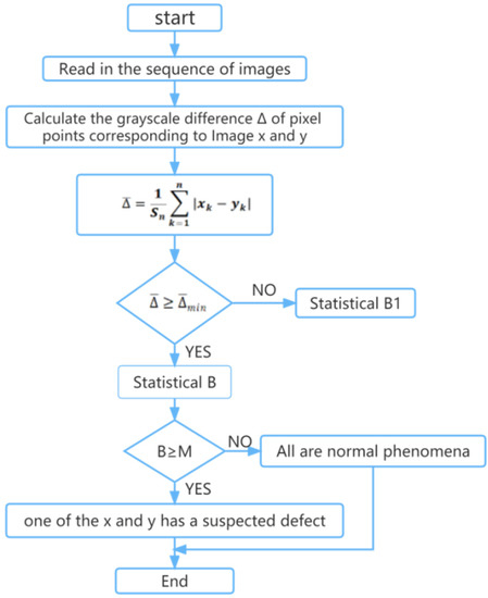
Figure 3.
PE gas pipeline defect screening algorithm.
2.3. Images Enhancement for Pipe Defects
Image enhancement is the process of enhancing an image’s display by highlighting its edges and significant texture details and suppressing the display of unimportant areas. This somewhat enhances the image’s visual impact [26] or highlights some “useful” and compresses other “useless” information in the image. In this paper, global histogram equalization (Figure 4B1–B3), adaptive histogram equalization (Figure 4C1–C3), and gamma transform (Figure 4D1–D3) was applied to enhance the image of the grayscale (Figure 4A1–A3).
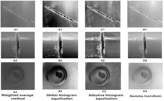
Figure 4.
Comparison of pipeline defect image enhancement effect.
Figure 4 illustrates that after the gamma transform, the defect image is not distorted; additionally, the defect’s edges become more noticeable and stand out against the background with a greater difference. In order to increase the contrast between the background of the pipe and the pipe defects, gamma transform was applied.
2.4. Pipe Defect Images Filtering and Denoising
During image transmission, the final image is often received with a lot of noise due to the interference of the environment or the limitations of the equipment. Image denoising is a classical image recovery task aiming to predict clean images from noisy observations [27]. Bilateral filtering (Figure 5B1–B3), Gaussian filtering (Figure 5C1–C3), mean filtering (Figure 5D1–D3), and adaptive median filtering (Figure 5E1–E3) were applied in this paper to denoise the images obtained above (Figure 5A1–A3).
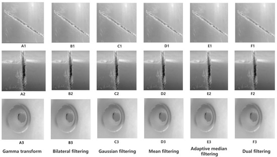
Figure 5.
Comparison of pipeline defect image filtering methods.
Step-by-step processing is a very common tactic for resolving complicated noisy images [28]. One of the weighted averages used for bilateral filtering is based on Gaussian distribution, which removes Gaussian noise from the image. However, the removal of Gaussian noise will ignore salt-and-pepper noise, and adaptive median filtering is the best algorithm to remove salt-and-pepper noise; however, it has poor results when removing Gaussian noise [24], Therefore, it was proposed to use dual filtering (Figure 5F1–F3) to remove the Gaussian noise by bilateral filtering after removing the salt-and-pepper noise by median filtering. Compared to other filtering algorithms, the dual filtering preserves the details of the edges and eliminates the noise points to achieve the effect of keeping the edges (as shown in Figure 5). Therefore, dual filtering was used for noise reduction in this paper.
3. Image Edge Detection and Segmentation for Pipe Defects
Image edges are the most basic feature of an image and using this feature the image can be segmented. In many imaging applications, it is sufficient to detect the periphery of an unknown object [29]. Image segmentation is usually performed before image feature quantization [30]. Threshold segmentation is a pixel-division technique used in region-based image segmentation, according to gray levels, into regions that have consistent properties, while neighboring regions do not have such consistent properties.
3.1. Improved Edge Detection with Sobel Operator
The conventional Sobel operator first performs a weighted average process for each pixel using a convolutional template (shown in Figure 6) and then acquires the gradient values in the X and Y directions by performing a difference process. It is challenging for the algorithm to achieve the desired detection results and the localization accuracy is not satisfactory, because the prevalent Sobel algorithm is just sensitive to the X directions and Y directions and can only assess the edges in both X directions and Y directions [24]. Various shapes and depths of the PE gas pipeline defects lead to negligible regional variations in the grayscale of the deficiency images; the collected images of PE gas pipeline defects contain a lot of interference data because of compression and real-time transmission. It is ineffective and very likely to result in missing edges, relying solely on two directional templates to identify the edges of pipe defects. In order to detect edge pixels in images more accurately, the Sobel algorithm was improved to eight directions [31] (as in Figure 7), which not only detects image edges more effectively but also increases edge detection accuracy and lowers the likelihood of incorrect edges.
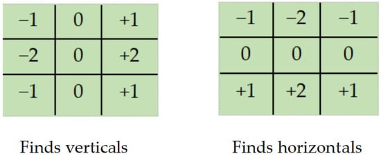
Figure 6.
Sobel operator template.
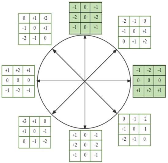
Figure 7.
Improved Sobel operator.
For the pipe defect filtered image obtained above (Figure 8A1–A3), the improved Sobel algorithm (Figure 8B1–B3), the Sobel edge detection algorithm (Figure 8C1–C3) and the Prewitt algorithm (Figure 8D1–D3) are used for edge detection of the image, respectively. Figure 8 displays the outcomes of the three defects’ edge detection. According to the comparison study, the improved Sobel algorithm extracts defect edges with more continuity and integrity and can completely display the defect shape characteristics. Therefore, the improved Sobel algorithm was used for edge detection in this paper.
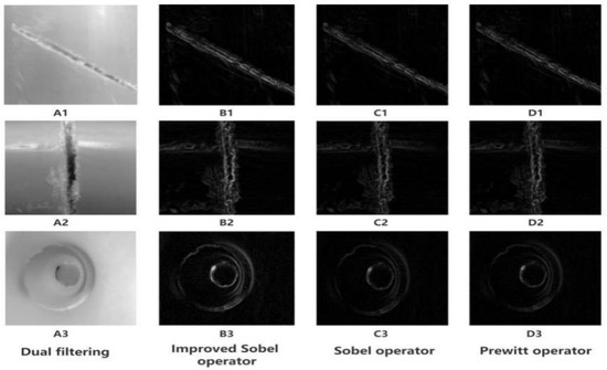
Figure 8.
Comparison of pipeline defect image edge detection.
3.2. Adaptive Threshold Segmentation
In the case of inhomogeneous illumination or uneven distribution of gray values, the segmentation results obtained if global threshold is used are often unsatisfactory, and adaptive threshold (also called local segmentation) can produce good results [32]. Adaptive threshold segmentation does not use one threshold for the whole matrix as a global threshold, but has a corresponding threshold for each value at each position of the input matrix.
The images (Figure 9A1–A3) present a comparison after the above edge detection was processed by adaptive threshold (Figure 9B1–B3), global threshold (Figure 9C1–C3) and Otsu threshold segmentation (Figure 9D1–D3), respectively. According to visual observation, an adaptive threshold can be used to distinguish pipeline defects from the pipe background, with the best segmentation of PE gas pipeline defects, with complete edge segmentation and less disturbing information. Therefore, the adaptive threshold algorithm was used to segment the image in this paper.
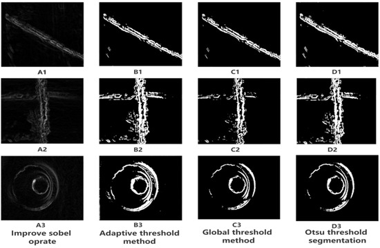
Figure 9.
Comparison of pipeline defect image threshold methods.
3.3. Morphological Operation
The shape of features in an image is typically the focus of morphological operation. It has been applied to eliminate defects in a variety of shapes with the purpose of smoothing the contours and preserving the object’s size and shape [33]. Erosion and dilation are the two main operations.
Let f(m,n) be the input image and g(m,n) be a structure element, If the set of real integers is denoted by Z, while assuming that (m,n) is an integer f(m,n) from Z*Z, g(m,n) is a function of a pixel’s gray value with the given coordinates (m,n) and the gray value is also an integer. Namely, g(m,n) to f(m,n) for grayscale dilation can be defined as , which is shown as Equation (7).
Equation (7) Df, Dg is the definition domain of f(m,n) and g(m,n), respectively, g(m,n) is the structural element of the morphological treatment is also a function, the displacement parameters (s − m), (t − n) must be in the definition domain of the function f(m,n).
The dilation operation is to find the local maximum value, and the anchor point is assigned the maximum of pixels in the nucleus coverage area. The erosion operation is to find the local minimum value. The minimum value of the pixel in the kernel coverage area is assigned to the anchor point. Erosion of grayscale image is defined as Equation (8).
Equation (8) Df, Dg is the definition domain of f(m,n) and g(m,n), respectively, g(m,n) is the structural element of the morphological treatment is also a function, the displacement parameters (s + m), (t + n) must be in the definition domain of the function f(m,n).
The expressions for the opening operation and closing operation of the grayscale image have the same form as the erosion and dilation, and the structural element g(m,n) performing the opening operation on the image f(m,n) can be defined , in Equation (9).
The opening operation is an erosion operation of g(m,n) on f(m,n) followed by an dilation operation on the result of the erosion. A similar closing operation of g(m,n) on f(m,n) can be defined in Equation (10).
In addition to the above operations, there is the morphological gradient operation; let the gradient be denoted by h in Equation (11).
The basic morphological operations: closed operation (Figure 10B1–B3), dilation (Figure 10C1–C3), erosion (Figure 10D1–D3), morphological gradient (Figure 10E1–E3), and opening operation (as in Figure 10F1–F3) are applied to the threshold segmentation image obtained above (Figure 10A1–A3) to compare the results. As shown in Figure 10, The opening operation’s result is to remove the image area that is slightly relative to the structure element and keeping the image area that is larger than the structure element [34]. The open operation more fully preserves the overall impact, and in this paper, we use the opening operation to fill the contours of defects in the images.
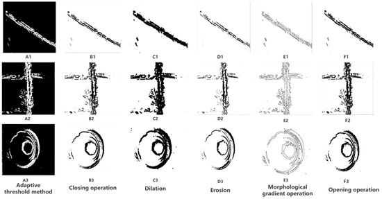
Figure 10.
Comparison chart of different morphological operations.
4. CNN-Based Image Defect Classification
The CNN’s primary characteristic is that its front-end input obtains image information by using multiple layers of locally interconnected neurons. The CNN can extract view invariant features [35] and takes full account of the translation, rotation, and scaling in space. Deep learning and convolutional networks have greatly improved the capability of target detection and classification using images. In this paper, three classification models, VGG16, Resnet50 and the original CNN model, are used for comparison, and the corresponding network structures are shown in Figure 11.
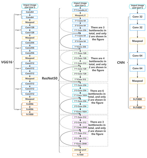
Figure 11.
Comparison of three network structures.
4.1. Classification Model
VGG16 has 16 layers, including 3 fully-connected layers, 5 pooling layers, and 13 convolutional layers. Resnet50 has 50 layers, including 1 fully-connected layer, 2 pooling layers, and 49 convolutional layers. The original CNN has 6 layers, including 2 fully-connected layers, 2 pooling layers, and 4 convolutional layers. The pooling layer is not counted as a pooling layer when determining the number of layers in the network because it has no parameters.
4.2. Convolutional Layer
The convolutional layer’s function is to extract the data from the source image, also referred to as image features. In the CNN architecture, the convolutional layer is typically the first layer, and the weight (wij) controls it, where i and j are the number of input and output feature mappings, respectively [36]. Thus, the entire convolution process can be defined, as in Equation (12).
In Equation (12), denotes the 2D convolution operation, aj is the set of input feature maps, bj denotes the jth underlying feature map, and denotes the activation function. In the CNN, each individual convolution layer performs a linear transformation from its input to the output representation through a multichannel multidimensional convolution operation. The convolution can be represented as a matrix–vector product, where the linear transform matrix is derived from the convolution filter and the vector represents the reshaped input of the layer [37].
4.3. Pooling Layer
The pooling layer’s primary function is to use specific factors to downsample the input feature mapping size, the average pool averages the features in the neighborhood to produce a blurring effect [38]. Spatial invariance can be attained by the pooling layer by lowering the feature map’s resolution. Each feature map that has been combined corresponds to a feature map from the layer before. Their cells combine inputs from a small block of n × n cells. The size of the pooling window is flexible, and the windows may overlap [39]. In this paper, maximum pooling is used.
4.4. Fully Connected Layer
Each feature matrix from the pooling layer is converted by the fully connected layer into a single column feature macrovector of dimension 1 × m [40]. The most common layer in a neural network is the fully connected layer, and each of its nodes is connected to each node in the previous and next layer. The dimensionality may increase, decrease, or remain constant during the transformation process [41]. In a convolutional neural network structure for classifying images, the fully connected layer is typically placed at the very end, and for better fitting the nonlinear problem, three fully connected layers are used in this paper. The VGG16 framework is shown in Figure 12.
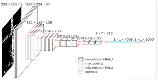
Figure 12.
VGG16 framework structures.
4.5. Classification Results
This project was developed using Python and the TensorFlow API, and the graphics card used for training, verification, and testing was an NVIDIA 2080TI, 32GB, DDR4. Each training run is 100 epochs (as shown Figure 13). In this paper, to evaluate the classification effectiveness of the model, the precision and recall of our confusion matrix were applied. Equations (13) and (14) give their definitions, where, respectively, TP, FP, and FN stand for true positives, false positives, and false negatives.
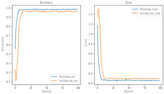
Figure 13.
Accuracy and loss function of VGG16 model.
Three types of pipe defect images, 100 of each were randomly selected for each defect as a test set from Table 1, Table 2 and Table 3, made evident that the VGG16 model’s recognition accuracy has improved significantly, particularly for cracks and fractures in the pipe body, where the recognition accuracy can reach an average of 98.5%, while the accuracy rate of holes is relatively low, but still can reach about 94%. From the confusion matrix (as shown in Figure 14), as can be seen, the classification algorithm in this paper has successfully identified three different types of defects with an average recognition rate of 97%. Compared with 94.96% percent of Xie et al. [36], the accuracy rate of this article has been improved by 2.04%. Compared with the 96.3% percent of Cong et al. [24], the accuracy rate of this article has been improved by 0.7%, which can be applied to the engineering practice of pipe defect detection and classification.

Table 1.
VGG16 defect classification results.
Table 2.
Resnet 50 defect classification results.
Table 3.
CNN defect classification results.
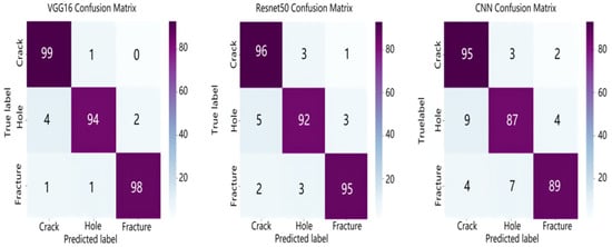
Figure 14.
Comparison of three algorithms confusion matrix.
5. Conclusions
This paper proposes a framework for classifying and identifying defects of underground PE gas transmission pipes. Fast and accurate detection of defects in PE pipelines is made possible through experimental verification. The following are the main results of this experiment.
- Based on the similarity of images of continuous pipelines, the images were first grayed out using the weighted average method and then preliminary screening of the acquired images was conducted to identify images with suspected defects, which improved the acquisition efficiency of defect image. For the defective PE gas pipeline images, contrast was enhanced using gamma transform, and finally noise was removed using the dual filtering method. The results show that the pre-processing technique can speed up image processing while retaining much of the detail of the originals.
- In order to detect the edges of image defects, an improved Sobel algorithm was presented. An adaptive thresholding segmentation method was used to segment the defects in the image. Then, after morphologically processing the image to obtain a binary image, the feature parameters of the defects were extracted.
- The obtained binary images were trained using VGG16, and the classifier was completed by selecting appropriate parameters for classification of various defects in images of the PE gas pipes. The experimental test results reveal that the highest accuracy of the classification approach adopted in this paper is 97% and it can be used not only for the identification of defective types of underground PE gas transmission pipes, but also for steel pipes, cast iron pipes, etc.
Author Contributions
Conceptualization, Y.W.; data curation, Q.F.; formal analysis, Y.W. and N.L.; funding acquisition, Y.W.; investigation, Y.W. and T.E.; methodology, N.L.; project administration, Y.W.; resources, Y.W. and N.L.; software, N.L.; supervision, Y.W. and H.L.; validation, H.Z.; visualization, Q.F.; writing—original draft, Q.F. and H.Z.; writing—review and editing, T.E. and H.L. All authors have read and agreed to the published version of the manuscript.
Funding
This research was funded by the National Natural Science Foundation of China (no. 11903072), the Xinjiang University Doctoral Start-up Foundation (no. 620321029) and the Science and technology planning project of State Administration for Market Regulation (no. 2022MK201).
Institutional Review Board Statement
Not applicable.
Informed Consent Statement
Not applicable.
Data Availability Statement
The data presented in this study are available on request from the corresponding author. The data are not publicly available.
Acknowledgments
The authors wish to thank all the reviewers who participated in the review during the preparation of this manuscript.
Conflicts of Interest
The authors declare no conflict of interest.
Nomenclature
| x,y | consecutive images of any adjacent PE pipes in our pipe database |
| xk,yk | the grayscale discrepancy between the correspondent pixel locations of x, y |
| Sn | number of pixels in designated size region |
| u, v | coordinates of grayscale values |
| s,t | displacement parameters |
| m,n | the functions f and g are the corresponding coordinates |
| aj | represents the convolution operation |
| bj | represents the jth base feature map |
| activation function | |
| wij | weights |
| I(u,v) | grayscale values |
| f(m,n) | input image |
| g(m,n) | structural elements |
| dilation operation | |
| erosion operation | |
| opening operation |
References
- Bachir-Bey, T.; Belhaneche-Bensemra, N. Investigation of Polyethylene Pipeline Behavior after 30 Years of Use in Gas Distribution Network. J. Mater. Eng. Perform. 2020, 29, 6652–6660. [Google Scholar] [CrossRef]
- Zha, S.; Lan, H. Fracture behavior of pre-cracked polyethylene gas pipe under foundation settlement by extended finite element method. Int. J. Press. Vessel. Pip. 2021, 189, 104270. [Google Scholar] [CrossRef]
- Velázquez, J.C.; Hernández-Sánchez, E.; Terán, G.; Capula-Colindres, S.; Diaz-Cruz, M.; Cervantes-Tobón, A. Probabilistic and Statistical Techniques to Study the Impact of Localized Corrosion Defects in Oil and Gas Pipelines: A Review. Metals 2022, 12, 576. [Google Scholar] [CrossRef]
- Hou, Q.; Yang, D.; Li, X.; Xiao, G.; Ho, S.C.M. Modified leakage rate calculation models of natural gas pipelines. Math. Probl. Eng. 2020, 2020, 6673107. [Google Scholar] [CrossRef]
- Zheng, T.; Liang, Z.; Zhang, L.; Tang, S.; Cui, Z. Safety assessment of buried natural gas pipelines with corrosion defects under the ground settlement. Eng. Fail. Anal. 2021, 129, 105663. [Google Scholar] [CrossRef]
- Wu, J.; Bai, Y.; Fang, W.; Zhou, R.; Reniers, G.; Khakzad, N. An Integrated Qu-antitative Risk Assessment Method for Urban Underground Utility Tunnels. Reliab. Eng. Syst. Saf. 2021, 213, 107792. [Google Scholar] [CrossRef]
- Sun, X.; Gu, J.; Tang, S.; Li, J. Research progress of visual inspection technology of steel products—A review. Appl. Sci. 2018, 8, 2195. [Google Scholar] [CrossRef]
- Yin, X.; Chen, Y.; Bouferguene, A.; Zaman, H.; Al-Hussein, M.; Kurach, L. A deep learning-based framework for an automated defect det-ection system for sewer pipes. Autom. Constr. 2020, 109, 102967. [Google Scholar] [CrossRef]
- Meijer, D.; Scholten, L.; Clemens, F.; Knobbe, A. A Defect Classication Methodology for Sewer Image Sets with Convolutional Neural Networks. Autom. Constr. 2019, 104, 281–298. [Google Scholar] [CrossRef]
- Liu, H.; Hou, L.; Luo, Z.; Zhou, Y.; Jing, X.; Truong, T.-K. Image Recovery with Data Missing in the Presence of Salt-and-Pepper Noise. Appl. Sci. 2019, 9, 1426. [Google Scholar] [CrossRef]
- Zhuang, P.; Li, C.; Wu, J. Bayesian retinex underwater image enhancement. Eng. Appl. Artif. Intell. 2021, 101, 104171. [Google Scholar] [CrossRef]
- Houssein, E.H.; Helmy, E.D.; Elngar, A.A.; Abdelminaam, D.S.; Shaban, H. An improved tunicate swarm algorithm for global optimization and image segmentation. IEEE Access 2021, 9, 56066–56092. [Google Scholar] [CrossRef]
- Zhang, B. Reconfigurable Morphological Processor for Grayscale Image Processing. Electronics 2021, 10, 2429. [Google Scholar] [CrossRef]
- Zhou, M.; Pan, Z.; Liu, Y.; Zhang, Q.; Cai, Y.; Pan, H. Leak Detection and Location Based on ISLMD and CNN in a Pipeline. IEEE Access 2019, 7, 30457–30464. [Google Scholar] [CrossRef]
- Ma, D.; Liu, J.; Fang, H.; Wang, N.; Zhang, C.; Li, Z.; Dong, J. A Multi-defect detection system for sewer pipelines based on StyleGAN-SDM and fusion CNN. Constr. Build. Mater. 2021, 312, 125385. [Google Scholar] [CrossRef]
- Hosseinzadeh, S.; Jackson, W.; Zhang, D.; McDonald, L.; Dobie, G.; West, G.; MacLeod, C. A Novel Centralization Method for Pipe Image Stitching. IEEE Sens. J. 2020, 21, 11889–11898. [Google Scholar] [CrossRef]
- Song, H.; Ge, K.; Qu, D.; Wu, H.; Yang, J. Design of in-pipe robot based on inertial positioning and visual detection. Adv. Mech. Eng. 2016, 8, 1687814016667679. [Google Scholar] [CrossRef]
- Chen, K.; Hu, H.; Chen, C.; Chen, L.; He, C. An intelligent sewer defect detection method based on convolutional neural network. In Proceedings of the IEEE International Conference on Information and Automation (ICIA), Wuyishan, China, 11–13 August 2018. [Google Scholar]
- Girshick, R. Fast R-CNN. In Proceedings of the International Conference on Computer Vision, Santiago, Chile, 7–13 December 2015; IEEE Computer Society: Washinton, DC, USA, 2015. [Google Scholar]
- Liu, W.; Anguelov, D.; Erhan, D.; Szegedy, C.; Reed, S.; Fu, C.; Berg, A.C. Ssd: Single shot multibox detector. In Proceedings of the European Conference on Computer Vision, Amsterdam, The Netherlands, 11–14 October 2016; Springer: Cham, Switzerland, 2016; pp. 21–37. [Google Scholar]
- Redmon, J.; Divvala, S.; Girshick, R.; Farhadi, A. You only look once: Unified, real-time object detection. In Proceedings of the IEEE Conference on Computer Vision and Pattern Recognition, Las Vegas, NV, USA, 27–30 June 2016. [Google Scholar] [CrossRef]
- Zhang, Y. The design of glass crack detection system based on image preprocessing technology. In Proceedings of the IEEE 7th Joint International Information Technology and Artificial Intelligence Conference, Chongqing, China, 20–21 December 2014. [Google Scholar]
- Jiang, Y.; Liu, Z.; Li, Y.; Li, J.; Lian, Y.; Liao, N.; Li, Z.; Zhao, Z. A Digital Grayscale Generation Equipment for Image Display Standardi-zation. Appl. Sci. 2020, 10, 2297. [Google Scholar] [CrossRef]
- Li, C.; Lan, H.-Q.; Sun, Y.-N.; Wang, J.-Q. Detection algorithm of defects on polyethylene gas pipe using image recognition-Science Direct. Int. J. Press. Vessel. Pip. 2021, 191, 104381. [Google Scholar] [CrossRef]
- Restivo, M.C.; Campbell-Washburn, A.E.; Kellman, P.; Xue, H.; Ramasawmy, R.; Hansen, M.S. A framework for constraining image SNR loss due to MR raw data compression. Magn. Reson. Mater. Phys. Biol. Med-Icine 2019, 32, 213–225. [Google Scholar] [CrossRef] [PubMed]
- Wu, H.; Zhou, Z. Partial Color Photo Processing Method for Components Based on Image Enhancement Technology. Wirel. Commun. Mob. Comput. 2021, 2021, 4132016. [Google Scholar] [CrossRef]
- Zhang, L.; Li, Y.; Wang, P.; Wei, W.; Xu, S.; Zhang, Y. A separation–aggregation network for image denoising. Appl. Soft Comput. 2019, 83, 105603. [Google Scholar] [CrossRef]
- Tian, C.; Fei, L.; Zheng, W.; Xu, Y.; Zuo, W.; Lin, C.-W. Deep learning on image denoising: An overview. Neural Netw. 2020, 131, 251–275. [Google Scholar] [CrossRef] [PubMed]
- Ren, H.; Zhao, S.; Gruska, J. Edge detection based on single-pixel imaging. Opt. Express 2018, 26, 5501–5511. [Google Scholar] [CrossRef]
- Cui, L.; Feng, J.; Zhang, Z.; Yang, L. High throughput automatic muscle image segmentation using parallel framework. BMC Bioinform. 2019, 20, 158. [Google Scholar] [CrossRef]
- Liu, W.; Wang, L. Quantum image edge detection based on eight-direction Sobel operator for NEQR. Quantum Inf. Process. 2022, 21, 190. [Google Scholar] [CrossRef]
- Liao, J.; Wang, Y.; Zhu, D.; Zou, Y.; Zhang, S.; Zhou, H. Automatic segmentation of crop/background based on luminance partition correction and adaptive threshold. IEEE Access 2020, 8, 202611–202622. [Google Scholar] [CrossRef]
- Abid Hasan, S.M.; Ko, K. Depth edge detection by image-based smoothing and morphological operations. J. Comput. Des. Eng. 2016, 3, 191–197. [Google Scholar] [CrossRef]
- Yang, M.D.; Su, T.C. Segmenting ideal morphologies of sewer pipe defects on CCTV images for automated diagnosis. Expert Syst. Appl. 2009, 36, 3562–3573. [Google Scholar] [CrossRef]
- Ben, X.; Zhang, P.; Lai, Z.; Yan, R.; Zhai, X.; Meng, W. A general tensor representation framework for cross-view gait recognition. Pattern Recognit. 2019, 90, 87–98. [Google Scholar] [CrossRef]
- Xie, Q.; Li, D.; Xu, J.; Yu, Z.; Wang, J. Automatic detection and classification of sewer defects via hierarchical deep learning. IEEE Trans. Autom. Sci. Eng. 2019, 16, 1836–1847. [Google Scholar] [CrossRef]
- Yi, X. Asymptotic Spectral Representation of Linear Convolutional Layers. IEEE Trans. Signal Process. 2022, 70, 566–581. [Google Scholar] [CrossRef]
- Singh, P.; Raj, P.; Namboodiri, V.P. EDS pooling layer. Image Vis. Comput. 2020, 98, 103923. [Google Scholar] [CrossRef]
- Scherer, D.; Müller, A.; Behnke, S. Evaluation of pooling operations in convolutional architectures for object recognition. In Proceedings of the International Conference on Artificial Neural Networks, Thessaloniki, Greece, 15–18 September 2010; Springer: Berlin/Heidelberg, Germany, 2010; pp. 92–101. [Google Scholar]
- Basha, S.H.S.; Dubey, S.R.; Pulabaigari, V.; Mukherjee, S. Impact of fully connected layers on performance of convolutional neural networks for image classification. Neurocomputing 2020, 378, 112–119. [Google Scholar] [CrossRef]
- Kalaycı, T.A.; Asan, U. Improving Classification Performance of Fully Connected Layers by Fuzzy Clustering in Transformed Feature Space. Symmetry 2022, 14, 658. [Google Scholar] [CrossRef]


Publisher’s Note: MDPI stays neutral with regard to jurisdictional claims in published maps and institutional affiliations. |
© 2022 by the authors. Licensee MDPI, Basel, Switzerland. This article is an open access article distributed under the terms and conditions of the Creative Commons Attribution (CC BY) license (https://creativecommons.org/licenses/by/4.0/).