
Drilling Parameters Optimization for Horizontal Wells Based on a Multiobjective Genetic Algorithm to Improve the Rate of Penetration and Reduce Drill String Drag

Abstract
:1. Introduction
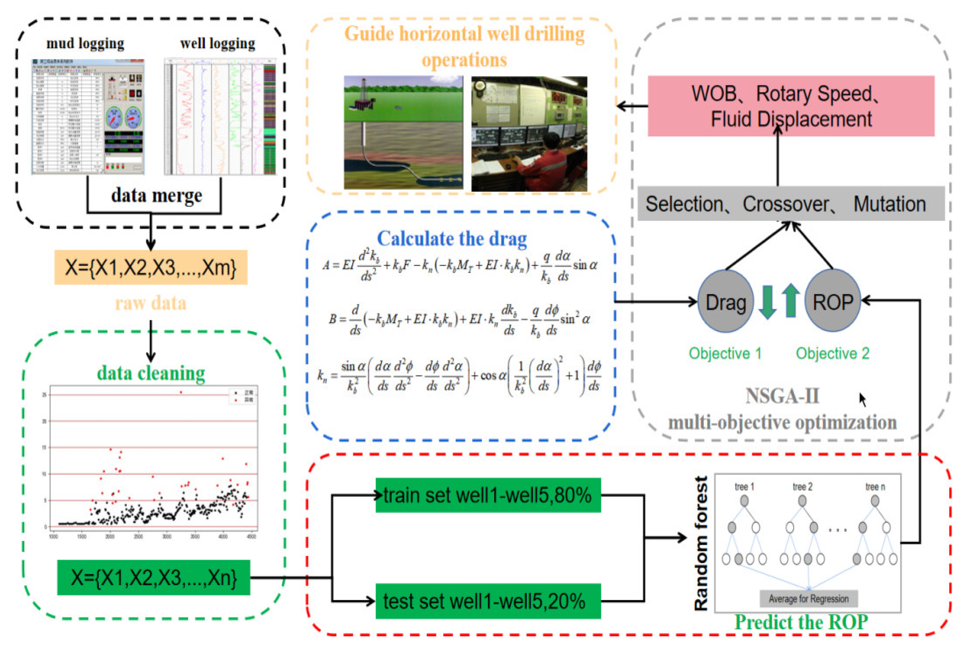
2. Data and Methods
2.1. Data
2.2. Data-Driven Algorithms
- (1)
- SVM algorithm
- (2)
- Random forest algorithm
- (3)
- Backpropagation (BP) neural network algorithm
2.3. The “Hard-String” Drag Calculation Method
2.4. Nondominant Sorting Genetic Algorithm-II
3. Results and Discussion
3.1. Abnormal Data Processing
3.2. Correlation Analysis between Drilling Parameters and ROP
3.3. Rate of Penetration Prediction Model
3.4. Drag Calculation Model
3.5. Multiobjective Collaborative Optimization Model
4. Conclusions
Author Contributions
Funding
Institutional Review Board Statement
Informed Consent Statement
Data Availability Statement
Acknowledgments
Conflicts of Interest
References
- Mo, H.; Shi, Z.; Hao, S.; Li, Q. Analysis and Application of Treatment Techniques in Horizontal Directional Drilling Borehole Accident. Procedia Earth Planet 2011, 3, 273–279. [Google Scholar] [CrossRef] [Green Version]
- Sha, L. Drilling Parameters Optimization Technology Status and Development Trend. China Pet. Mach. 2016, 44, 29–33. [Google Scholar] [CrossRef]
- Chen, X.; Gao, D.; Guo, B.; Feng, Y. Real-time optimization of drilling parameters based on mechanical specific energy for rotating drilling with positive displacement motor in the hard formation. J. Nat. Gas Sci. Eng. 2016, 35, 686–694. [Google Scholar] [CrossRef]
- Bahari, A.; Seyed, A.B. Drilling cost optimization in a hydrocarbon field by combination of comparative and mathematical methods. Pet. Sci. 2009, 6, 451–463. [Google Scholar] [CrossRef] [Green Version]
- Hankins, D.; Salehi, S.; Saleh, F.K. An integrated approach for drilling optimization using advanced drilling optimizer. J. Pet. Eng. 2015, 2015, 281276. [Google Scholar] [CrossRef] [Green Version]
- Hegde, C.; Daigle, H.; Gray, K.E. Performance comparison of algorithms for real-time rate-of-penetration optimization in drilling using data-driven models. SPE J. 2018, 23, 1706–1722. [Google Scholar] [CrossRef]
- Gray, K.E.; Hegde, C. Use of machine learning and data analytic to increase drilling efficiency for nearby wells. J. Nat. Gas Sci. Eng. 2017, 40, 327–335. [Google Scholar] [CrossRef]
- Momeni, M.; Hosseini, S.J.; Ridha, S.; Laruccia, M.B. An optimum drill bit selection technique using artificial neural networks and genetic algorithms to increase the rate of penetration. J. Eng. Sci. 2018, 13, 361–372. [Google Scholar]
- Abughaban, M.; Alshaarawi, A.; Meng, C. Optimization of drilling performance based on an intelligent drilling advisory system. In Proceedings of the International Petroleum Technology Conference, Beijing, China, 26–28 March 2019. [Google Scholar] [CrossRef]
- Payette, G.S.; Spivey, B.J.; Wang, L.; Bailey, J.R. Real-time well-site based surveillance and optimization platform fordrilling: Technology, basic workflows and field results. In Proceedings of the SPE/IADC Drilling Conference and Exhibition, The Hague, The Netherlands, 14–16 March 2017. [Google Scholar] [CrossRef]
- Gidh, Y.; Purwanto, A.; Bits, S. Artificial Neural Network Drilling Parameter Optimization System Improves ROP by Predicting/Managing Bit Wear. In Proceedings of the SPE Intelligent Energy International, Utrecht, The Netherlands, 27–29 March 2012. [Google Scholar] [CrossRef]
- Guria, C.; Goli, K.K.; Pathak, A.K. Multi-objective optimization of oil well drilling using elitist non-dominated sorting genetic algorithm. Pet. Sci. 2014, 11, 97–110. [Google Scholar] [CrossRef] [Green Version]
- Ammar, A.; Mahmoud, A.; Beshir, M. Hybrid data driven drilling and rate of penetration optimization. J. Pet. Sci. Eng. 2021, 200, 108075. [Google Scholar] [CrossRef]
- Omojuwa, E.; Osianya, S.; Ahmed, R. Influence of Dynamic Drilling Parameters on Axial Load and Torque Transfer in Extended-Reach Horizontal Wells. In Proceedings of the SPE Annual Technical Conference and Exhibition, Amsterdam, The Netherlands, 27–29 October 2014. [Google Scholar] [CrossRef]
- Wang, Z.; Wang, X.; Chen, L. Status and Prospect of Technologies to Reduce Cost and Increase Efficiency for Drilling in Bohai Oilfield. Xinjiang Oil Gas 2022, 18, 66–72. [Google Scholar]
- Bingham, M.G. A New Approach to Interpreting Rock Drillability; Petroleum Publishing Company: Tulsa, OK, USA, 1965. [Google Scholar]
- Bourgoyne, A.; Young, F.S. A multiple regression approach to optimal drilling and abnormal pressure detection. Soc. Pet. Eng. J. 1974, 14, 371–384. [Google Scholar] [CrossRef]
- Hareland, G.; Rampersad, P. Drag-bit model including wear. In Proceedings of the SPE Latin America/Caribbean Petroleum Engineering Conference, Buenos Aires, Argentina, 27–29 April 1994. [Google Scholar] [CrossRef]
- Al-abduljabbar, A. A robust rate of penetration model for carbonate formation. J. Energy Resour. Technol. 2019, 141, 042903. [Google Scholar] [CrossRef]
- Hegde, C.; Wallace, S.; Gray, K. Using trees, bagging, and random forests to predict rate of penetration. In Proceedings of the SPE Middle East Intelligent Oil and Gas Conference and Exhibition, Abu Dhabi, UAE, 15–16 September 2015. [Google Scholar] [CrossRef]
- Chiranth, H.; Hugh, D.; Harry, M. Analysis of rate of penetration (ROP) prediction in drilling using physics-based and data-driven models. J. Pet. Sci. Eng. 2017, 159, 295–306. [Google Scholar] [CrossRef]
- Su, X.; Sun, J.; Gao, X.; Wang, M. Prediction method of Drilling rate penetration based on GBDT algorithm. Comput. Appl. Softw. 2019, 36, 87–92. [Google Scholar]
- Ashrafi, S.B.; Anemangely, M.; Sabah, M.; Ameri, M.J. Application of hybrid artificial neural networks for predicting rate of penetration (ROP): A case study from Marun oil field. J. Petrol. Sci. Eng. 2019, 175, 604–623. [Google Scholar] [CrossRef]
- Soares, C.; Gray, K. Real-time predictive capabilities of analytical and machine learning rate of penetration (ROP) models. J. Pet. Sci. Eng. 2019, 172, 934–959. [Google Scholar] [CrossRef]
- Hassan, A.; Elkatatny, S.; Al-Majed, A. Coupling rate of penetration and mechanical specific energy to Improve the efficiency of drilling gas wells. J. Nat. Gas Sci. Eng. 2020, 83, 103558. [Google Scholar] [CrossRef]
- Song, X.; Pei, Z.; Wang, P.; Zhang, G. Intelligent Prediction for Rate of Penetration Based on Support Vector Machine Regression. Xinjiang Oil Gas 2022, 18, 14–20. [Google Scholar]
- Ahmed, O.S.; Adeniran, A.A.; Samsuri, A. Computational intelligence based prediction of drilling rate of penetration: A comparative study. J. Pet. Sci. Eng. 2019, 172, 1–12. [Google Scholar] [CrossRef]
- Breiman, L. Random Forests. Mach. Learn. 2001, 45, 5–32. [Google Scholar] [CrossRef] [Green Version]
- Zhu, S.; Song, X.; Li, G. Intelligent real-time drag and torque analysis and sticking trend prediction of drill string. Oil Drill. Prod. Technol. 2021, 43, 428–435. [Google Scholar] [CrossRef]
- Ho, H.-S. An Improved Modeling Program for Computing the Torque and Drag in Directional and Deep Wells. In Proceedings of the SPE Annual Technical Conference and Exhibition, Houston, TX, USA, 2–5 October 1988. [Google Scholar] [CrossRef]
- Deb, K.; Pratap, A.; Agarwal, S.; Meyarivan, T.A.M.T. A fast and elitist multi-objective genetic algorithm: NSGA-II. IEEE Trans. Evol. Comput. 2002, 6, 182–197. [Google Scholar] [CrossRef]
- Boslaugh, S. Statistics in a Nutshell: A Desktop Quick Reference; O’Reilly Media Inc.: Boston, MA, USA, 2012. [Google Scholar]


| Work | Obj. Function | Opt. Parameters |
|---|---|---|
| Abughaban et al. [9] | max ROP, min MSE | WOB, RPM |
| Payette et al. [10] | max ROP, min stick–slip risk | WOB, RPM, GPM |
| Gidh et al. [11] | max ROP, max bit life | WOB, RPM |
| Guria et al. [12] | max ROP, max bit life | WOB, RPM, PP |
| Ammar et al. [13] | max ROP, min nonproductive time (NPT) | WOB, RPM, GPM |
| Data Sources | Features |
|---|---|
| Mud logging | Depth, rate of penetration (ROP), weight on bit (WOB), handing load, revolutions per minute (RPM), torque(T), pumping flow per minute (GPM), equivalent density of drilling fluid |
| Well logging | Well deviation, azimuth, acoustic logging, density logging |
| Bit parameters | Diameter, cutting-tooth diameter, number of cutting tooth |
| Work | Equation | Coefficients |
|---|---|---|
| Bingham [16] | ||
| B and Y [17] | ||
| Hareland [18] | ||
| Al-abduljabbar [19] |
| Model | Hyperparameter Type | Value |
|---|---|---|
| RF | number of decision trees | 185 |
| maximum depth of decision tree | 130 | |
| minimum number of samples required to split decision tree nodes | 2 | |
| finding the optimal number of feature variables to consider for a node | 9 | |
| impurity evaluation function | MSE | |
| SVM | kernel function | rbf |
| penalty parameter | 100 | |
| gamma parameter | 0.01 | |
| BP | number of hidden layers | 3 |
| number of neurons | [64, 128, 32] | |
| optimizer | Adam | |
| learning rate | 0.001 | |
| loss function | MSE |
| Hyperparameters Type | Value |
|---|---|
| number of individuals in each population | 20 |
| number of population iterations | 25 |
| probability of individual crossover | 0.7 |
| probability of individual mutation | 0.2 |
| Depth (m) | Values | WOB (kN) | RPM (r/min) | GPM (l/min) | ROP (m/h) | Improve | Drag (kN) | Reduce |
|---|---|---|---|---|---|---|---|---|
| 1181 | Initial | 206.3 | 60.5 | 25.0 | 18.26 | 16.31% | 47.2 | 4.0% |
| Recommended | 188.2 | 66.8 | 27.0 | 21.24 | 45.3 | |||
| 1591 | Initial | 95.4 | 61.2 | 34.0 | 20.08 | 12.50% | 53.5 | 3.0% |
| Recommended | 89.5 | 68.0 | 37.0 | 22.59 | 51.9 | |||
| 2304 | Initial | 85.2 | 52.5 | 38.0 | 15.11 | 12.37% | 104.7 | 0.1% |
| Recommended | 80.0 | 59.2 | 42.0 | 16.98 | 103.6 | |||
| 3004 | Initial | 144.9 | 56.0 | 43.0 | 10.23 | 19.66% | 118.2 | 7.0% |
| Recommended | 133.2 | 63.0 | 46.0 | 12.22 | 109.9 | |||
| 3636 | Initial | 170.0 | 48.2 | 48.0 | 3.26 | 19.63% | 120.6 | 5.0% |
| Recommended | 163.0 | 56.8 | 52.0 | 3.9 | 114.6 |
Publisher’s Note: MDPI stays neutral with regard to jurisdictional claims in published maps and institutional affiliations. |
© 2022 by the authors. Licensee MDPI, Basel, Switzerland. This article is an open access article distributed under the terms and conditions of the Creative Commons Attribution (CC BY) license (https://creativecommons.org/licenses/by/4.0/).
Share and Cite
Zang, C.; Lu, Z.; Ye, S.; Xu, X.; Xi, C.; Song, X.; Guo, Y.; Pan, T. Drilling Parameters Optimization for Horizontal Wells Based on a Multiobjective Genetic Algorithm to Improve the Rate of Penetration and Reduce Drill String Drag. Appl. Sci. 2022, 12, 11704. https://doi.org/10.3390/app122211704
Zang C, Lu Z, Ye S, Xu X, Xi C, Song X, Guo Y, Pan T. Drilling Parameters Optimization for Horizontal Wells Based on a Multiobjective Genetic Algorithm to Improve the Rate of Penetration and Reduce Drill String Drag. Applied Sciences. 2022; 12(22):11704. https://doi.org/10.3390/app122211704
Chicago/Turabian StyleZang, Chuanzhen, Zongyu Lu, Shanlin Ye, Xinniu Xu, Chuanming Xi, Xianzhi Song, Yong Guo, and Tao Pan. 2022. "Drilling Parameters Optimization for Horizontal Wells Based on a Multiobjective Genetic Algorithm to Improve the Rate of Penetration and Reduce Drill String Drag" Applied Sciences 12, no. 22: 11704. https://doi.org/10.3390/app122211704