Investigation and Design of the Transonic Laminar Flow Characteristics in a Laminar Aircraft

Abstract

Reducing drag is critical to aircraft design. In recent years, laminar technology has become one of the most important feasible technologies for civil aircraft drag reduction design under many design constraints. However, various factors have a certain impact on the laminar flow characteristics in the state of transonic flight. Therefore, it is necessary to deeply understand the specific effects of various flight parameters on the characteristics of laminar flow. In this paper, a parameter sensitivity analysis for a central experimental wing in a special layout aircraft was carried out to investigate its transonic laminar characteristics. Then, the airfoil of the central experimental wing of the aircraft was designed for real flight. The RANS (Reynold-averaged Navier–Stokes) method combined with the $\gamma -{\mathrm{Re}}_{\theta }$ transition model based on local variables was used. The computational approach was validated by the wind tunnel tests and analyzed by the grid independence analysis. The sensitivity mainly focuses on the transition location and the length of the laminar flow zone of the central experiment under different boundary conditions. The transonic transition was affected by a variety of interacting factors that include FSTI (free stream turbulence intensity), pressure gradient, Re (Reynolds number), Ma (Mach number) and α (angle of attack, degree). The essence of the transition is the disruption of flow stability caused by the increase in flow entropy. Among these factors, FSTI directly affects global flow stability, and the pressure gradient affects local flow stability. Ma and α can indirectly affect the flow stability by changing the pressure gradient. Re can control the boundary layer properties to change the flow stability, whereas its effect is easily determined by the pressure gradient. Finally, the improved design of the airfoil with the central experimental wing was conducted. The design of weak shock wave and aerodynamic load on the rear part of the airfoil can improve the aerodynamic characteristics (C_L, lift coefficient, increases by 0.28) of the airfoil, which can reduce the load burden on the outboard wing without affecting the laminar flow characteristics of the airfoil. In the next step, cross-flow instability will be considered.

1. Introduction

With the increasing depletion of petroleum resources, environmental protection and emission reduction have attracted more and more attention. The International Air Transport Association has set new requirements for the aviation industry to reduce emissions and noise. For civil airliners, reducing engine power, which is mainly used to overcome the drag of aircraft flight, is an important way to reduce emissions [1]. In the zero-lift drag of the aircraft, the form drag and frictional drag generally each account for 50% [2]. When the aerodynamic layout of the aircraft is determined, the form drag may not be changed greatly, while the skin frictional drag may still be drastically reduced [3]. Since the frictional drag of the laminar boundary layer is much smaller than that of the turbulent boundary layer, expanding the zone of the laminar flow on the surface of the aircraft is one of the most effective methods to reduce the frictional drag, which is called Laminar drag reduction technology. By appropriate contour design or the use of some flow control techniques, a C_p (pressure coefficient) curve can be created that favors flow stabilization and delays or suppresses transitions.

Laminar drag reduction technology is one of the most important feasible technologies for civil aircraft drag reduction design under many design constraints [4]. It has become one of the major study objectives of aircraft designers. The surface finish of the wing was low due to the limited capacity of early aviation manufacturing in the past century. At the same time, the antifouling and deicing technologies on the wing surface are also not mature [5]. Therefore, the laminar flow characteristics of the aircraft were not obvious. At present, laminar flow design has gradually become possible with the advancement of design technology and the manufacturing process in the aviation industry. For civil aircraft, NLF (natural laminar flow) technology can maintain a laminar flow state with about 60% of the chord length on the airfoil at low speeds (around Mach Number 0.2) and with about 40% of the chord length on the airfoil at high speeds (around Mach Number 0.78). If NLF technology is adopted by the whole aircraft, the frictional drag can be reduced by about 30%, and the drag of the whole aircraft can be reduced by more than 15% [6,7,8]. This aerodynamic benefit is very obvious and more economical. Moreover, the reduction in fuel consumption greatly reduces carbon emissions, which is conducive to reducing air pollution.

NASA (National Aeronautics and Space Administration), DLR (Deutsches Zentrum für Luft- und Raumfahrt), and ONERA started research on NLF technology in the 1980s. They achieved a series of results that have been applied to Boeing757 and A320 [9,10,11]. The Japanese “Honda jet” adopted the NLF wing and NLF fuselage head design and achieved the expected goals and requirements on the first flight in 2003 [12,13]. Northwestern Polytechnical University developed an e^N transition prediction method based on the linear stability theory and studied the infinitely stretched wing and the hybrid laminar wing–body combination [14,15]. China Aerodynamics Research and Development Center carried out some calibration and application research based on the transition model $\gamma -{\mathrm{Re}}_{\theta }$ [16]. Beihang University applied Walters and Menter’s methods, respectively, to the transition prediction of hypersonic flow [17]. A comparison of the two methods for hypersonic boundary layer transition prediction was accomplished via sharp cone at different Re and HIFiRE-5shape. Results have proven that both the k-ω-γ transition model and the “laminar+transition criteria” model can predict correct transition onsets and lengths at different Reynolds numbers but fail to predict the heat overshoot observed in experimental results. In recent years, the research of NLF technology has been further developed. In 2017, NASA proposed the NLF design method that addressed transition due to attachment line contamination/transition, Gortler vortices, cross-flow and Tollmien-Schlichting modal instabilities [18]. NASA and Boeing also conducted natural laminar flow tests on wings and studied the effect of TS (Tollmien–Schlichting) and cross-flow waves on the transition at different Reynolds numbers based on the common research model in the National Transonic Facility and European Transonic Wind tunnel wind tunnels in the US in 2018 [19,20]. In 2019, Zhen-Ming Xu et al. proposed to explain the mechanism by CFPG (examining cross-flow pressure gradient). Their finding suggested that we should pay more attention to the control of CFPG when designing an NLF forward-swept wing towards suppression of cross-flow instability to maintain extensive NLF [21]. At the same time, the effects of the angle of attack and Reynolds number on the Common Research Model with Natural Laminar Flow extent were studied, and the dominant transition mechanism was evaluated at a variety of test conditions by NASA [22]. In 2020, Airbus et al. designed the BLADE (Breakthrough Laminar Demonstrator in Europe) aircraft. The aircraft basis for the experimental aircraft is an A340-300 Flight Test aircraft from which the outer wings were replaced with carefully designed NLF panels of a lower sweep. Additionally, the correlation of data from a range of different test instrumentation provides a comprehensive analysis of the sensitivities of NLF, demonstrating the effectiveness of the BLADE platform [23]. In 2022, experiments with laminar boundary layer suction in adverse pressure gradient were performed on a wing in a wind tunnel. It was proven that applying boundary layer suction can lead to a drag reduction of up to 30% when compared with the no suction condition [24]. In the same year, the wind tunnel and flight tests of a natural laminar flow wing glove were simulated and analyzed by the numerical simulation method considering transition judgment by Wang H et al. 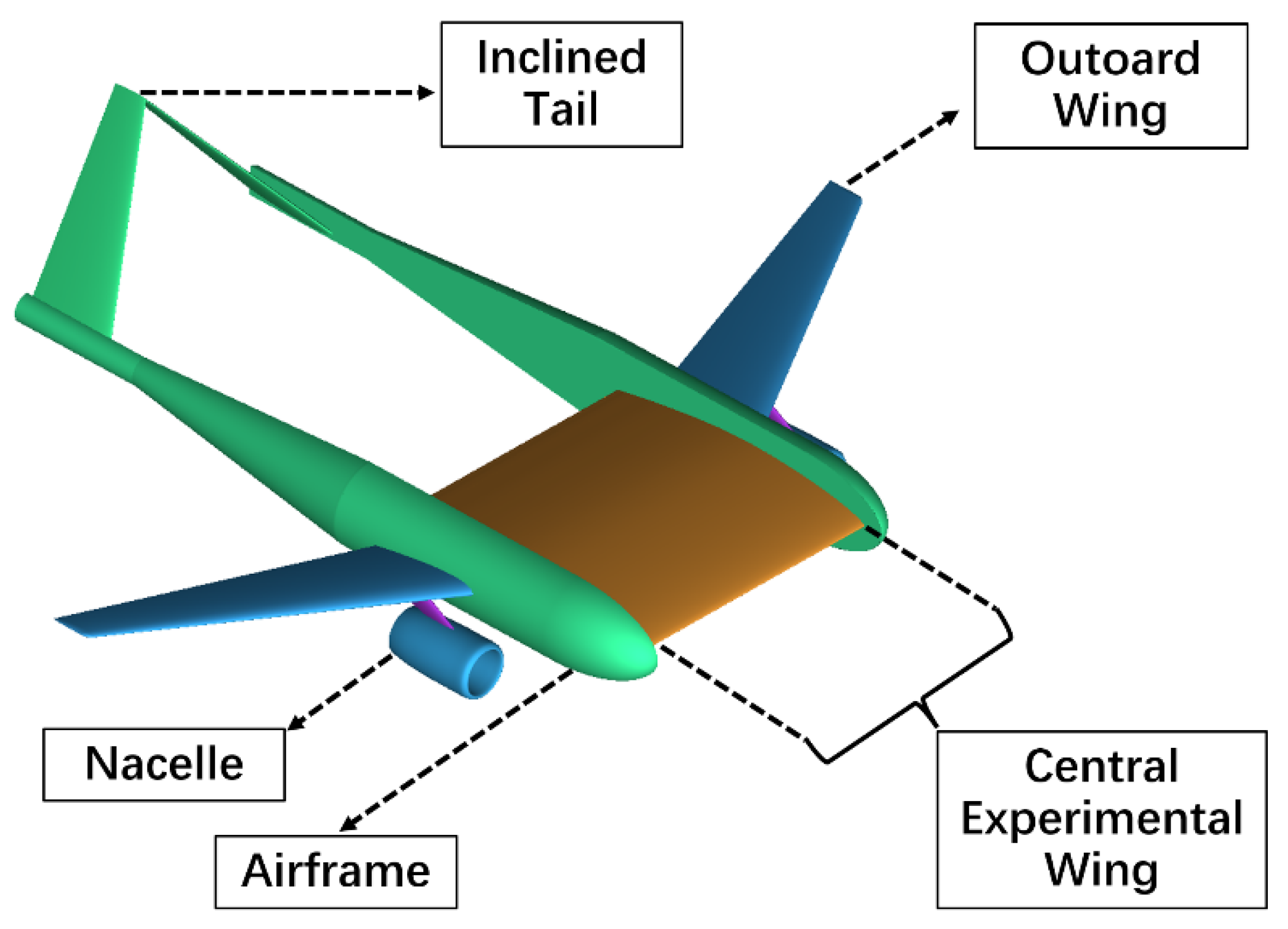[25]. It was found that the transition position obtained by numerical simulation in the design stage and the typical non-design state of the wing glove are in good agreement with the flight test results. Therefore, at present, NLF technology is mainly verified by numerical simulation computing and wind tunnel test. Some flight test verification of NLF technology has also been conducted. However, the NLF area of these flight tests is obtained by an NLF wing glove installed on the wing of the aircraft. There are the following shortcomings in this test flight mode. Firstly, the design of the NLF wing glove is subject to the limitations and constraints of the wing itself. The design space is reduced, which affects the diversity of NLF tests. Secondly, traditional flight verification aircraft use manned aerial vehicles generally, so the higher risk of test flights is compared to unmanned aerial vehicles. Finally, the cost of a traditional test flight is high. There is an urgent practical need to use new specially designed aircraft for the flight verification of laminar flow technology. Therefore, a special layout aircraft shown in Figure 1 was designed by the first aircraft institute of the Aviation Industry Corporation of China. The aircraft adopts a modular design that the central experimental wing can be replaced according to the experimental requirements. Only the central experimental wing was used for the laminar flow experiment, and the outboard wing section and airframe did not participate in the experiment. The outboard wing section provides lift, and the central experimental wing is responsible for conducting a laminar flow test. It is a UAV (unmanned aerial vehicle) with a lower flight cost. Therefore, the flight test design is more flexible to further study the laminar flow mechanism, provide more efficient and low-cost flight verification data and shorten the period of laminar flow wing design.

This article mainly qualitatively studies the effects of various sensitive factors on laminar flow characteristics to provide a reliable reference for the design and test flight of the laminar flow verification aircraft. It also provides a source of data for future studies on the differences between flight tests and numerical simulations.

As is known, the key to laminar flow technology is to control the boundary layer transition. The boundary layer transition has a significant impact on the development of the boundary layer, frictional drag and flow separation position. The characteristics of the transonic boundary layer were studied in the 1960s. H. H. Pearcey et al. gave a review of NACA wind-tunnel measurements of the pressure fluctuations at the surfaces of aerofoils and in their wakes. These observations show that large fluctuations may occur under the conditions for which separation would be expected [26]. In 1980, A theoretical analysis was made to determine the real-gas effects on the simulation of transonic boundary layers in wind tunnels with cryogenic nitrogen as the test gas by Jerry B. Adock et al.. The results indicate that the adiabatic cryogenic–nitrogen boundary layers are not substantially different from ideal-gas boundary layers, with the maximum difference of the various boundary layer parameters being on the order of one percent [27]. Additionally, in 1985, Deepak Om et al. conducted a series of experiments to explore transonic shock-wave/turbulent boundary-layer interactions. They found that the interaction depends very strongly on the Mach number, but the effect of the Reynolds number on the interaction is small [28]. These studies mainly focus on qualitative analysis and interpretation of the characteristics of the transonic boundary layer because the ability to extract test data from the boundary layer is poor. Until recently, Boeing proposed BLDS (boundary layer data system) for commercial jet aircraft surface flow measurements in the transonic flight regime in 2016. Evaluations of boundary layer data quality and comparisons between the in-flight measured boundary layer velocity profile data and numerical simulation results are shown for the wing and vertical tail survey locations. The measurements and computations agree closely at lower Mach numbers. For the highest Mach numbers, there is general agreement for overall thickness, but some differences between predicted and measured profile shape details remain for the wing boundary layer. In general, it provides a better data extraction method for the in-depth study of transonic boundary layer characteristics [29]. In 2022, Ardhendu Chakraborty et al. investigated controlling transonic shock boundary layer interactions over a natural laminar flow airfoil by vortical and thermal excitation. The research on flow control by thermal and vortical excitations shows the relative advantage of the latter over the former [30]. Thus, the characteristics of the transonic boundary layer are still complex, especially the effects of various conditions on it, such as Ma and Re. The Re also has an important influence on the transition. Prediction of laminar flow and accurate assessment of drag requires consideration of turbulence models and transition effects [31,32]. In short, various factors have a certain impact on the laminar flow characteristics in the state of transonic flight. Therefore, it is necessary to deeply understand the specific effects of various flight parameters on the characteristics of laminar flow. However, wind tunnel experiments are difficult to accurately reflect the laminar flow characteristics in the real flight state because of the influence of wind tunnel wall interference and the Reynolds number effect in wind tunnels. Although the three-dimensional laminar flow sensitivity based on swept-back wings may have been analyzed by many, the interaction between the sensitivity factors has rarely been studied, which is one of the novelties of this paper.

In this paper, a preliminary study of the transonic laminar flow characteristics in real flight conditions was carried out based on this aircraft using CFD (computational fluid dynamics) methods. Additionally, the airfoil of the central experimental wing was designed to reduce the load burden on the outboard wing without affecting the experimental study of the central experimental wing. This will provide a reference for the subsequent laminar flow study. The detailed research process is as follows: Firstly, the RANS method combining the transition prediction model $\gamma -{\mathrm{Re}}_{\theta }$ based on local variables and the wind tunnel tests was used to analyze the transonic laminar flow parameter sensitivity for the aircraft. The RANS-based transition prediction method was validated and analyzed by the wind tunnel tests. Through the comparative analysis of numerical simulation results of the central experimental wing of the laminar flow aircraft and the corresponding test data, the calculation ability and accuracy of the transition prediction method were verified. The numerical simulation research in this paper focused on the laminar characteristics near the cruise state, the transition position of the central experimental wing and the length of the laminar flow zone of the central experimental wing under different flight states. Through the calculation, the influence of key flow parameters such as FSTI (free stream turbulence intensity), Re (Reynolds number), Ma (Mach number) and α (angle of attack, degree) on the transition position of the airfoil surface was summarized. Finally, to conduct high-speed laminar flight experiments, the aircraft design needs to consider the coordination of the aerodynamic characteristics between the outboard wing and the central experimental wing. There is a large area in the central experimental wing, so the reasonable design of the wing can reduce the load burden of the outboard wing without affecting the laminar flow experimental study. Therefore, based on the sensitive investigation, an improved design of the airfoil of the central experimental wing was carried out. In the future, the central experimental wing models based on forward-swept wings and backward-swept wings with different airfoils will be further studied to reveal more complex laminar flow mechanisms deeply.

2. Computational Approach

2.1. Numerical Methods

The governing equations in this paper are the RANS (Reynold-averaged Navier–Stokes) equations. The finite volume method was applied to solve the RANS equations. The second-order upwind Roe-FDS (flux differences splitting) scheme was applied to discretize the inviscid spatial term, and the second-order central difference scheme was applied to discretize the viscous spatial. The transition model used in this paper is the four-equations $\gamma -{\mathrm{Re}}_{\theta }$ transition model based on the $k-\omega$ SST (shear stress transport) model [33,34]. The model uses the parameter γ to modify the generation and destruction terms of the turbulent kinetic energy equation in the standard two-equations $k-\omega$ SST model to simulate the transition process. The time-stepping method was the AF (approximate factorization) implicit time-marching method. In this method, the momentum equations for the contravariant velocity components and the elliptic equation for the pressure are solved directly in the transformed space by applying the delta-form approximate-factorization scheme and the Tschebyscheff method, respectively [35]. In order to accelerate convergence, the multi-grid method was applied. The multi-grid method is a general numerical technique for solving continuous problems such as boundary value problems or functional integral equations. There are many separate aspects and extensions of the method, and the study of multi-grid is an active area of numerical analysis research [36].

2.2. Grid Independence Verification

The grid is generated by ANSYS ICEM. The specific grid generation process is as follows: Firstly, the 3D grid block of the aircraft wall was cut out, as shown in Figure 2a. Then the external O-BLOCK function was used to generate the boundary layer mesh of the aircraft. In the boundary layer, the two adjacent grid nodes’ size growth rate was 1.15. The grid structure of the aircraft is shown in Figure 2b. Finally, the surface and volume grids, as shown in Figure 2c, were generated. A characteristic inflow and outflow boundary condition was applied. All solid surfaces were set as the no-slip adiabatic wall. The symmetry boundary condition was used to generate only a half-model grid. All calculation domains are calculated by RANS equations. A grid convergence study was applied to ensure the reliability of the numerical solution. Since the aircraft model is symmetric, the calculation was performed by half-mode to improve the computational efficiency.

The experimental aircraft with a laminar flow wing was calculated using six levels of the meshes shown in Figure 3 with the boundary condition in

Table 1. Boundary conditions of grid independence verification.

Computational Model	Ma	α (°)	Re	FSTI (%)
$\gamma -{\mathrm{Re}}_{\theta }$	0.70	2	1.1 × 107	0.2%

. It can be seen from Figure 3b that the main 2D grid size of the central experimental wing surface is 0.032 m × 0.028 m. $\gamma -{\mathrm{Re}}_{\theta }$ represents the transition model. Ma represents the Mach Number. α represents the angle of attack. Re represents the Reynolds Number. FSTI represents the free stream turbulence intensity. The first cell height condition is shown in

Table 2. First cell height condition.

Mesh Number	1	2	3	4	5	6
First cell height (meter)	20 × 10−6	10 × 10−6	5 × 10−6	2.5 × 10−6	1.25 × 10−6	0.625 × 10−6

. The growth ratio near the boundary layer, such as the ratio between Mesh 1 and Mesh 2, was 2, from 3.1 million volume grids to 120 million volume grids. The aerodynamic forces coefficient results are shown in Figure 4, in which the mesh number represents the mesh number. Mesh 6 is the finest grid, Mesh 1 is the coarsest grid, C_L represents the lift coefficient, C_D represents the drag coefficient and C_M represents the pitch moment coefficient. The results indicated that the aerodynamic characteristics of the six grids have little difference, so the grid independence is verified. When the number of volume cells was approximately 13.0 million (Mesh 3), the y+ is closest to 1, shown in Figure 5b. Y⁺ is a non-dimensional number similar to the local Reynolds number, determining whether the influences in the wall-adjacent cells are laminar or turbulent [37]. It is well known that Y⁺ ≈ 1 should be guaranteed when studying the boundary layer flow. Thus we chose Mesh 3 for subsequent calculation.

2.3. Comparison of CFD Results with Wind Tunnel Data

The experiment was carried out by the FL-2 wind tunnel in AVIC (Aerodynaiviics Research Institute of China). The FL-2 wind tunnel is a high-speed wind tunnel for a laminar experiment. The experiment adopted a 1:9.8 scale model, Ma = 0.7, Re = 8 × 10⁶, sideslip angle = 0°, FSTI = 0.6%. The FSTI specified at an inlet can decay quit rapidly depending on the inlet viscosity ratio (and hence turbulence eddy frequency). As a result, the local FSTI downstream of the inlet can be much smaller than the inlet value. Typically, the larger the inlet viscosity ratio, the smaller the turbulent decay rate. However, if too large a viscosity ratio is specified (i.e., >100), the skin friction can deviate significantly from the laminar value. There is experimental evidence that suggests that this effect occurs physically; however, at this point, it is not clear how accurately the transition model reproduces this behavior. For this reason, if possible, it is desirable to have a relatively low (i.e., =10) inlet viscosity ratio and to estimate the inlet value of FSTI such that at the leading edge of the wall of the airfoil the FSTI has decayed to the desired value. The grid calculated in Section 2.2 was used to complete the comparison. Figure 6 shows the transition comparison between the experimental results of the wind tunnel and the calculated results when α = 0°and α = 1°. The left side of (a) and (b) are the calculated results of the skin friction coefficient of the central experimental wing, while the right side is the experimental thermographic image. It can be seen from the experimental thermographic image that the transition zone of the central experimental wing presents a zigzag feature, which is different from the smooth transition zone presented by the calculation result. It is because the surface of the experimental model has a certain degree of roughness, which leads to the advance of the local transition. Thus, the experimental transition position is taken as the maximum chordwise distance that can be achieved in the laminar flow zone. It can be seen that at α = 0°and α = 1°, the transition positions of the calculated results (x/c = 56.2% at α = 0°and x/c = 54.8% at α = 1°) are consistent with the experimental results. The positions of the transition in the calculated results and the experimental results advance as the angle of attack increases. Figure 7a shows the C_p curve measured by PSP (pressure-sensitive pain) on the upper airfoil of the original laminar airfoil at the airfoil section Y/Span = 5%. C_p represents the pressure coefficient, EXP. represents the experimental result and CAL. represents the calculated result. It can be seen from Figure 7a that the experimental C_p is slightly higher near the leading edge, while the C_p of other positions is slightly lower than the calculated value. This is because there is a certain difference between the thickness of the airfoil processed in the experiment and that of the calculated model. The coating on the surface may also have a certain influence. However, the experimental curve and the calculated curve show the same trend, which is enough that laminar flow characteristics require a favorable pressure gradient (negative pressure increases with chordwise distance). Figure 7b shows the C_L between the experimental results of the wind tunnel and the calculated results when α from 0° to 3°. It can be seen that the C_L curve of the calculated results is in good agreement with the experimental results. Through the above analysis, the CFD method used in this paper is reliable.

As shown in Figure 8, the transition mode in the case of the Re (around 10⁷) and β = 0° at the central experimental wing was mainly dominated by TS instability. There was no transition of cross-flow instability in the zone. The experimental wind tunnel was a low-turbulence degree wind tunnel, so the cross-flow traveling wave instability was not considered. For the instability dominated by cross-flow standing waves, the disturbance source was mainly the wall roughness. However, the experimental model in the laminar flow wind tunnel had a higher smoothness than the model in the wind tunnel for the measurement of aerodynamic coefficients. As a result, the laminar flow experimental model had a relatively high critical Re for cross-flow standing wave instability. This type of transition is not easy to occur. Therefore, the transition of cross-flow was not considered. In summary, the calculation method mentioned in the section is sufficient to simulate the laminar flow state studied in this paper.

3. Results and Discussion of Sensitivity Analysis

3.1. Sensitivity Analysis of FSTI

The calculated states of this section are shown in

Table 3. Calculated states and method for different FSTI.

Computational Model	Ma	α(°)	Re/×107	FSTI (%)
$\gamma -{\mathrm{Re}}_{\theta }$	0.70	2	1.1	0.2, 0.6, 1.0

. Y/Span represents the spanwise C_p curve section. The spanwise Cp curve sections are mainly 5%, 15% and 25% in Figure 9a. From the C_p calculation results in Figure 9, it can be seen that the variation in the FSTI has basically no effect on the C_p characteristics of the central experimental wing. On the contrary, from the calculation results of Figure 10 and Figure 11, the length of the laminar flow zone is influenced strongly by the FSTI. When FSTI is 0.2%, the transition position shown in Figure 10a (about 50% of the chord length from the leading edge of the central experiment wing) is near the starting point of the adverse pressure gradient shown in Figure 9a. When FSTI is 0.6%, the transition in Figure 10b (about 30% of the chord length from the leading edge of the central experiment wing) occurs in the weak favorable pressure gradient segment shown in Figure 9b. When FSTI is 1.0%, the transition position in Figure 10c (about 18% of the chord length from the leading edge of the central experiment wing) is near the strong stop point of the favorable pressure gradient shown in Figure 9c. The evidence from the above phenomenon suggests that the transition position varies mainly with the FSTI. At this time, the main factor affecting the transition is FSTI, and the existence of a laminar flow zone cannot be guaranteed by the weak favorable pressure gradient. The transition mode under different FSTI is the natural transition formed by the sudden Tollmien–Schlichting instability. Therefore, the favorable pressure gradient is not a sufficient condition for the maintenance of laminar flow. The increase in FSTI leads to a significant advance in the transition position at each station in the spreading direction. The transition positions at each Y/Span are significantly advanced due to the increase in the FSTI. The most obvious finding to emerge from this section is that FSTI has a strong destructive effect on the maintenance of the laminar zone of the wing, and the greater FSTI, the more likely TS instability occurs.

3.2. Sensitivity Analysis of Re

The calculated states of this section can be seen in

Table 4. Calculated states and method for different Re.

Computational Model	Ma	α (°)	Re/×107	FSTI (%)
$\gamma -{\mathrm{Re}}_{\theta }$	0.70	2	0.550, 0.825, 1.100, 1.350, 1.650, 2.000	0.2

. Figure 12 shows that the C_p of different Re is basically the same. The C_p characteristics show a slight difference at 60% chord length only at Re 5.5 × 10⁶. Therefore, when the magnitude of Re is about 10⁷, Re has little effect on the C_p curve. For general attachment flow, the magnitude of the Re affects the thickness of the boundary layer on the aircraft surface, as shown in Figure 13, the skin friction coefficient reflected in Figure 14, the transition location of the boundary layer displayed in Figure 15, and the flow separation related to the viscosity. The boundary layer thickness was obtained by extracting the velocity of the flow field grid nodes. Boundary layer thickness refers to the height perpendicular to the wall from the boundary layer wall to the position where the tangential flow velocity along the wall reaches 99% of the free flow velocity. In Figure 14 and Figure 15, the effect of the variation in Re on the transition position has an obvious nonlinear characteristic. The increase in Re leads to a regular advancement of the transition position during the range of Re between 5.50 × 10⁶ and 1.35 × 10⁷. The advanced degree of the transition position also increases with the Re increase, and the transition occurs at the starting point of the adverse pressure gradient and in the weak favorable pressure gradient segment. This is because the boundary layer becomes thinner with the increase in Re, which leads to a decrease in flow stability. The flow that encounters disturbance near the airfoil surface is more likely to become turbulent from laminar flow. Eventually, the transitional position gradually approaches the strong stop point of favorable pressure gradient with rapid TS instability. However, when the Re is greater than 1.35 × 10⁷, the increase in the Re has little effect on the advance of the transition position. This is mainly because the transition position has gradually approached the strong stop point of the favorable pressure gradient of the central experimental wing. The flow of the boundary layer has obtained enough energy to maintain the stability of laminar flow under the influence of a strong forward pressure gradient, even though the boundary layer has become thinner due to the increase in the Re. The transition position advance degree reaches the limit as the degree of entropy increase is restricted by the strong forward pressure gradient. As a result, the dominant transition factor is changed from the increase in Re to a strong forward pressure gradient. The transition is not easy to advance further. In short, the effect of Re on the transition position is easily overridden by the strongly favorable pressure gradient of the C_p distribution, and the sensitivity priority of Re is low.

3.3. Sensitivity Analysis of Ma

The calculated states of this section are listed in

Table 5. Calculated states and methods for different Ma.

Computational Model	Ma	α (°)	Re/×107	FSTI (%)
$\gamma -{\mathrm{Re}}_{\theta }$	0.61, 0.64, 0.67, 0.70, 0.73, 0.76, 0.79	2	1.1	0.2

. As shown in Figure 16, the variation in Ma has a very obvious effect on the C_p characteristics of the central experiment wing. As the Ma increases, the C_p shifts upward around 50% chard shifts upward and forms a shock wave finally. However, the variation in the transition position with the Ma increase is different with C_p. In Figure 17 and Figure 18, the effect of Ma on the laminar flow zone has an obvious nonlinear character. The airfoil surface laminar zone length is the longest when the Ma is 0.70. The transition occurs in the segment of transformation from the favorable pressure gradient to the adverse pressure gradient. The transition mode is the natural transition by the gradual instability of the TS. When the Ma decreases from 0.7 to 0.61, the airfoil transition position is advanced. The transition mode is sudden TS instability. As the Ma increases from 0.70 to 0.79, the negative pressure peak on the central experiment wing gradually increases with the appearance of a shock wave. The C_p curves become irregular in the 30% to 70% chord with alternating adverse pressure gradient and favorable pressure gradient. Hence, because a stable weak shock wave is caused by the increase in Ma, the changes in the transition position are relatively small within a small range and show a high degree of nonlinearity. The transition occurs in the weak favorable pressure gradient segment, not in the strong adverse pressure gradient segment after the shock wave. The transition mode is the natural transition. In short, the increased favorable pressure gradient due to the increase in Ma is beneficial to the extension of laminar flow length. However, when the shock wave has been formed, the pressure gradient is stable. The tendency of laminar zone extension disappears with the increase in Ma. It is worth noting that the design of the laminar flow wing is great. Because the design of cruise Ma is 0.7, the laminar flow zone in the central experimental wing will be stable when the Ma is greater than or equal to the design of cruise Ma.

3.4. Sensitivity Analysis of α

The calculated states of this section are listed in

Table 6. Calculated states and method for different α.

Computational Model	Ma	α (°)	Re/×107	FSTI (%)
$\gamma -{\mathrm{Re}}_{\theta }$	0.70	0, 2, 4	1.1	0.2

. From the results in Figure 19, Figure 20 and Figure 21, it is found that all the effects of increasing α on the characteristics of the C_p curves and the transition position have a strong regularity. The positive direction of α is shown in the coordinate system in Figure 20. As α increases, the favorable pressure gradient on the upper surface becomes small, gradually shown in Figure 19, and the transition position is gradually advanced, reflected in Figure 20 and Figure 21. When the α increases from 0°to 4°, the transition position is advanced from approximately 57% to 30% of the chord of the central experimental wing. The change in α affects the laminar flow characteristics by affecting the shape of the favorable pressure gradient at the front of the C_p curves (the segment from 0% to 30% of the chord). From Figure 19a,b, it can be observed that the two adverse pressure gradient zones form as the α increases to 4°, while the transition occurs near the start point of the first adverse pressure gradient. This indicates that the laminar flow zone is very sensitive to the adverse pressure gradient. A small local adverse pressure gradient is possible to cause TS instability. In short, decreasing α has a beneficial effect on expanding the length of the laminar flow zone but decreases the lift of aircraft. The trade-off between lift and laminar flow needs to be decided by the aircraft designer. Expanding the length of the laminar flow zone on the wing surface to reduce drag as much as possible while lift requirements are still met.

Finally, the process and interrelationship of each sensitivity factor are shown in Figure 22. The direction of the arrow represents the affected object, and the width of the arrow line represents the influence weight.

The transonic transition is affected by a variety of interacting factors that include pressure gradient, FSTI, Re, Ma, α, etc. FSTI affects global flow stability, and its effect is not easily overridden by other factors. The transition position advances with increasing FSTI. The pressure gradient affects local flow stability. Especially the favorable pressure gradient is a landmark factor of local transition but not necessarily a decisive factor in maintaining the local laminar flow zone under transonic conditions. In most cases, a larger favorable pressure gradient zone implies a larger laminar flow zone. However, once the values of FSTI and Re are too extreme, the relationship between the length of the favorable pressure gradient and the laminar zone length is not clear. Re affects the flow stability indirectly by changing the characteristics of the boundary layer. Its increase leads to an earlier transition, but its effect is easily covered by the strongly favorable pressure gradient. The effect of Ma on the transition is highly nonlinear and affects the transition mainly by changing the pressure gradient. Its effect on the transition is divided into two phases. The first phase has no shock wave. In this process, as the Ma increases, the favorable pressure gradient zone gradually extends with the delaying of the transition and the appearance of the tendency to form a shock wave. In the second phase, the shock wave has been formed. The pressure gradient is more stable than the first phase. Therefore, it is difficult for the Ma increase to affect the transition position. α affects the transition location by changing the pressure gradient. Increasing α causes the transition to advance. In short, the essence of the transition is the disruption of flow stability caused by the increase in flow entropy. FSTI affects global flow stability, while pressure gradient affects local flow stability. Re, Ma and α indirectly affect the flow stability, and among them, Re is easily determined by the pressure gradient.

4. Results and Discussion of Airfoil Design

4.1. The Design of Airfoil

The purpose of the design is to improve the aerodynamic characteristics of the central experimental wing without affecting the laminar flow characteristics. OLD represents the original laminar flow airfoil, while NEW represents the design airfoil based on OLD.

On the one hand, Ma and α are the two most likely factors to change in a specific aircraft’s high-speed flight condition. Through the sensitivity analysis in Section 3, it is known that the Ma and the α directly affect the pressure gradient and the original airfoil of the central experimental wing adopts a no-shock wave design. The advantage of this design, shown in Figure 23, is that the aerodynamic characteristics at the design point are excellent. However, once the boundary conditions deviate from the design point, the aerodynamic characteristics deteriorate rapidly. In contrast, the weak shock wave design is more commonly used in aerodynamic designs, whose overall robustness displayed in Figure 23 is better than the other one. Additionally, better aerodynamic characteristics can be maintained in a wide range. This is beneficial for investigating the laminar flow characteristics under a relatively wide range of boundary conditions. If the C_p curve is less robust, the stability of the pressure gradient will be poor. The pressure gradient with poor stability results in highly nonlinear laminar flow characteristics, which will make it difficult to summarize the experimental law. Therefore, the weak shock wave design is more suitable for the C_p curve design of the airfoil in the central experimental wing. On the other hand, to increase the C_L/C_D characteristic in cruise, the airfoil trailing edge curvature is increased to increase the local rear loading of C_L, which can improve the C_L aircraft and the C_L/C_D under the same C_L without affecting the laminar flow characteristic. (The C_L of the whole aircraft increases, resulting in a reduction in the cruising α. The decrease in cruise α leads to a decrease in C_D, so the C_L/C_D increases.) Based on the above design analysis, the following three design improvements were made to the original laminar flow airfoil shown in Figure 24:

• The airfoil curve from 50% chord length to 70% chord length on the upper surface of the airfoil is adjusted to slightly reduce the local airfoil thickness to promote the formation of weak shock waves;
• The maximum thickness position of the lower surface of the airfoil is shifted forward by 10% to increase the region of aerodynamic load on the rear part of the airfoil;
• The curvature of the trailing edge of the lower surface of the airfoil is reversed and increased to promote the formation of aerodynamic load on the rear part of the airfoil. This increases the nose-down pitching moment. Thus, this should be limited for structural and trim.

Figure 23. Comparison with and without weak shock wave.

Figure 23. Comparison with and without weak shock wave.

Figure 24. Result of airfoil design.

Figure 24. Result of airfoil design.

4.2. Design Results

The calculated states used by OLD and NEW are listed in

Table 7. Boundary conditions of the airfoil design.

Computational Model	Ma	α (°)	Re	FSTI (%)
$\gamma -{\mathrm{Re}}_{\theta }$	0.70	0, 1, 2	1.1 × 107	0.2%

. The results of the C_p curve in the central experimental wing are displayed in Figure 25. These results show that a weak shock wave appears at 50% chord length of the NEW airfoil at α = 2°. The C_p shape in front of the shock wave of the NEW does not change significantly compared with the C_p curve of OLD. However, the value of C_p decreases, which benefits the increase in the C_L. The position of the negative pressure peak is moved from 60% to 50% of the chord direction, which further increases the aerodynamic load on the rear part of the airfoil. The aerodynamic load after a 50% chordwise position on the lower surface of the NEW airfoil is obvious. Therefore, the whole area enclosed by the C_p curve is significantly increased. In short, the shape of the C_p curve matches well with the design intent. In addition, the favorable pressure gradient segment from the leading edge of the airfoil to 50% of the chord length on the OLD upper surface is well inherited by NEW. This determines the laminar flow characteristics of the NEW on the upper surface. It can be found in Figure 26 that the length of the laminar flow zone of NEW does not change significantly in comparison with the OLD. It is worth noting that there is no difference at all in the transition positions of the OLD and NEW airfoil types at α = 0°. When α is 1° or 2°, a slight delay in the transition position of NEW is produced in comparison with OLD. Because the weak shock wave design slightly extends the length of the favorable pressure gradient segment of the airfoil, increasing the flow stability in front of the shock wave. Therefore, the laminar flow characteristics are slightly improved when the shock wave appears.

Through the analysis above, the prerequisite of the design of this chapter inheriting the laminar flow characteristics is well achieved. The transition position is not advanced by airfoil design. From the C_L curve shown in Figure 27a, the C_L has a more obvious increase after the aerodynamic load on the rear part of the airfoil increases. The C_L increases by about 0.28 in the range of 0°to 3°of α, which greatly reduces the load burden on the outboard wing. This will provide a reference for laminar aircraft design. The C_D pole curve intuitively shows the improvement of the lift-drag characteristics near the cruise α = 1°after increasing the aerodynamic load on the rear part of the airfoil. Although the NEW has the larger nose-down pitch moment compared to the OLD, about 0.08, this increment has little effect on the flat tail trim of the aircraft.

5. Conclusions

In this paper, a parameter sensitivity analysis for a special layout laminar aircraft with a central experimental wing is carried out to investigate the transonic laminar characteristics. The airfoil of the central experimental wing of the aircraft is designed for the flight experiment. Based on the comparison and analysis of the results, several important conclusions are drawn as follows:

(1)

The transonic transition is affected by a pressure gradient, FSTI, Re, Ma, α, etc. The effect of FSTI is not easily overridden by other factors. The pressure gradient affects local flow stability. In most cases, a larger favorable pressure gradient zone implies a larger laminar flow zone. Once the values of FSTI and Re are too extreme, the relationship between the length of the favorable pressure gradient and the laminar zone length is not clear. Re affects the flow stability indirectly by changing the characteristics of the boundary layer. Its increase leads to an earlier transition, but its effect is easily covered by the strongly favorable pressure gradient. The effect of Ma on the transition is highly nonlinear and affects the transition mainly by changing the pressure gradient. Its effect on the transition is divided into two phases. The first phase has no shock wave. In this process, as the Ma increases, the favorable pressure gradient zone gradually extends with the delaying of the transition and the appearance of a tendency to form a shock wave. In the second phase, the shock wave has been formed. The pressure gradient is more stable than the first phase, so it is difficult for the Ma increase to affect the transition position. α affects the transition location by changing the pressure gradient. Increasing α will cause the transition to advance. In short, the essence of the transition is the disruption of flow stability caused by the increase in flow entropy. FSTI affects global flow stability, while pressure gradient affects local flow stability. Re, Ma and α indirectly affect the flow stability, and among them, Re is easily determined by the pressure gradient;

(2)

The design of weak shock waves and aerodynamic load on the rear part of the airfoil effectively improves the lift characteristics of the central experimental wing. C_L increases by 0.28, which reduces the load burden on the outboard wing without affecting the laminar flow characteristics of the central experimental wing. It should be noted that this design idea is not only for the OLD laminar flow airfoil, but this conclusion can also be used as a reference for designing the same type of laminar flow experimental aircraft. Because real flight conditions are much more complex than wind tunnel tests, the aircraft designer must do everything possible to optimize the performance of the aircraft.

These results can not only help designers obtain a better understanding of the relationship between laminar characteristics and these sensitivity factors but also improve the laminar flow design by referring to the above conclusions.

References

1. Yu, G.; Li, D.; Zhang, Z. Numerical simulation for the differences between FTN/WPN engine models aerodynamic influence on BWB300 airframe. Eng. Appl. Comput. Fluid Mech. 2020, 14, 566–579. [Google Scholar] [CrossRef] [Green Version]
2. General Editorial Board of Aircraft Design Manual. Air Craft Design Manual (Volume 6): Aerodynamic Design; National Defense Industry Press: Beijing, China, 2002; pp. 252–322. [Google Scholar]
3. Lee, J.D.; Jameson, A. NLF airfoil and wing design by adjoint method and automatic transition prediction. In Proceedings of the 27th AIAA Applied Aerodynamics Conference, Reston, Virginia: AIAA, San Antonio, TX, USA, 22–25 June 2009; p. 3514. [Google Scholar]
4. Cameron, L.; Early, J.; Mcroberts, R. Metamodel assisted multi-objective global optimisation of natural laminar flow aerofoils. In Proceedings of the 29th AIAA Applied Aerodynamics Conference, Reston: AIAA, Honolulu, HI, USA, 27–30 June 2011; p. 3001. [Google Scholar]
5. Risse, K.; Schueltke, F.; Stumpf, E. Conceptual wing design methodology for aircraft with hybrid laminar flow control. In Proceedings of the 52nd Aerospace Sciences Meeting, National Harbor, MD, USA, 13–17 January 2014; p. 0023. [Google Scholar]
6. Lai, G.J.; Li, Z.D.; Zhang, Y.Z. Research on natural laminar airfoil wind tunnel test at high Reynolds number. Aeronaut. Sci. Technol. 2017, 28, 12–15. [Google Scholar]
7. Streit, T.; Horstmann, K.; Schrauf, G. Complementary numerical and experimental data analysis of the ETW telfona pathfinder wing transition tests. In Proceedings of the 49th AIAA Aerospace Sciences Meeting including the New Horizons Forum and Aerospace Exposition, Reston, Virginia: AIAA, Orlando, FL, USA, 4–7 January 2011; p. 881. [Google Scholar]
8. Vermeersch, O.; Yoshida, K.; Ueda, Y. Natural laminar flow wing for supersonic conditions: Wind tunnel experiments, flight test and stability computations. Prog. Aerosp. Sci. 2015, 79, 64–91. [Google Scholar] [CrossRef]
9. Kruse, M.; Wunderlich, T.; Heinrich, L. A conceptual study of a transonic NLF transport aircraft with forward swept wings. In Proceedings of the 30th AIAA Applied Aerodynamics Conference, Reston: AIAA, New Orleans, LA, USA, 25–28 June 2012; p. 3208. [Google Scholar]
10. Eppink, J.; Wlezien, R. Data analysis for the NASA/boeing hybrid laminar flow control crossflow experiment. In Proceedings of the 41st AIAA Fluid Dynamics Conference and Exhibit, Reston: AIAA, Honolulu, HI, USA, 27 June–30 June 2011; p. 3879. [Google Scholar]
11. Fauci, R.; Nicoli, A.; Imperatore, B. Wind tunnel tests of a transonic natural laminar flow wing. In Proceedings of the 25th AIAA Aerodynamic Measurement Technology and Ground Testing Conference, Reston: AIAA, Atlanta, GA, USA, 5–8 June 2006; p. 3638. [Google Scholar]
12. Fujino, M.; Yoshizaki, Y.; Kawamura, Y. Natural-laminar-flow airfoil development for a lightweight business jet. J. Aircr. 2003, 40, 609–615. [Google Scholar] [CrossRef]
13. Fujino, M. Design and development of the HondaJe. J. Aircr. 2005, 42, 755–764. [Google Scholar] [CrossRef]
14. Zhang, K.; Song, W.P. Application of the full en transition method to the infinite swept-wing’s transition prediction. J. Northwestern Polytech. Univ. 2011, 29, 142–147. [Google Scholar]
15. Zhu, Z.; Song, W.P.; Han, Z.H. Automatic transition prediction for wing-body configurations using dual eN method. Acta Aeronaut. Astronaut. Sin. 2018, 39, 121707. [Google Scholar]
16. Mou, B.; Jiang, X.; Xiao, Z.Y. Implementation and caliberation of γ-Re-θ transition model. Acta Aerodyn. Sin. 2013, 31, 103–109. [Google Scholar]
17. Zhou, L.; Yan, C.; Hao, Z.H. Transition model and transition criteria for hypersonic boundary layer flow. Acta Aeronaut. Astronaut. Sin. 2016, 37, 1092–1102. [Google Scholar]
18. Lynde, M.N.; Campbell, R.L. Computational design and analysis of a transonic natural laminar flow wing for a wind tunnel model. In Proceedings of the 35th AIAA Applied Aerodynamics Conference, Denver, CO, USA, 5–9 June 2017; p. 3058. [Google Scholar]
19. Lynde, M.N.; Campbell, R.L.; Rivers, M.B. Preliminary results from an experimental assessment of a natural laminar flow design method. In Proceedings of the AIAA Scitech 2019 Forum, San Diego, CA, USA, 7–11 January 2019; p. 2298. [Google Scholar]
20. Rivers, M.B.; Lynde, M.N.; Campbell, R.L. Experimental investigation of the nasa common research model with a natural laminar flow wing in the nasa langley national transonic facility. In Proceedings of the AIAA Scitech 2019 Forum, San Diego, CA, USA, 7–11 January 2019; p. 2189. [Google Scholar]
21. Xu, Z.; Han, Z.; Zhu, Z. On the Flow Mechanism of Forward Swept Natural-Laminar-Flow Wing for Crossflow Instability Suppression. In Proceedings of the AIAA Aviation 2019 Forum, Dallas, TX, USA, 17–21 June 2019; p. 3291. [Google Scholar]
22. Lynde, M.N.; Campbell, R.L.; Viken, S.A. Additional findings from the common research model natural laminar flow wind tunnel test. In Proceedings of the AIAA Aviation 2019 Forum, Dallas, TX, USA, 17–21 June 2019; p. 3292. [Google Scholar]
23. Gibson, T.; Soucheleau, B.; Rogers, N. BLADE-Natural Laminar Flow Flight Testing. Available online: https://www.icas.org/ICAS_ARCHIVE/ICAS2020/data/papers/ICAS2020_0220_paper.pdf (accessed on 6 September 2021).
24. Corelli Grappadelli, M.; Sudhi, A.; Radespiel, R. Experimental study of a wing with hybrid laminar flow control application. In Proceedings of the AIAA AVIATION 2022 Forum, Chicago, IL, USA, 27 June–1 July 2022; p. 3770. [Google Scholar]
25. Pearcey, H.H.; Holder, D.W. Examples of the Effects of Shock-Induced Boundary-Layer Separation in Transonic Flight. 1954. Available online: https://reports.aerade.cranfield.ac.uk/handle/1826.2/4088 (accessed on 25 January 1954).
26. Adcock, J.B.; Johnson, C.B. A Theoretical Analysis of Simulated Transonic Boundary Layers in Cryogenic-Nitrogen Wind Tunnels. 1980. Available online: https://ntrs.nasa.gov/api/citations/19800010854/downloads/19800010854.pdf (accessed on 12 March 1980).
27. Om, D.; Viegas, J.R.; Childs, M.E. Transonic shock-wave/turbulent boundary-layer interactions in a circular duct. AIAA J. 1985, 23, 707–714. [Google Scholar] [CrossRef]
28. Mejia, K.M.; Ulk, C.; Antunes, A.P. Testing of an Autonomous Boundary Layer Data System Device in the Transonic Flight Regime. In Proceedings of the 2018 Aerodynamic Measurement Technology and Ground Testing Conference, Atlanta, GA, USA, 25–29 June 2018; p. 4196. [Google Scholar]
29. Chakraborty, A.; Roy, A.G.; Sundaram, P. Controlling transonic shock–boundary layer interactions over a natural laminar flow airfoil by vortical and thermal excitation. Phys. Fluids 2022, 34, 085124. [Google Scholar] [CrossRef]
30. Wang, H.; Zhong, M.; Hua, J. Analysis of simulation and experiment results of a natural laminar flow flight test wing glove. Acta Aeronaut. Astronaut. Sin. 2022, 43, 526785. (In Chinese) [Google Scholar]
31. Yan, C.; Qian, Y.J.; Lian, Q.X. Viscous Fluid Mechanics; Beijing University of Aeronautics & Astronautics Press: Beijing, China, 2005; pp. 45–66. [Google Scholar]
32. Schlichting, H. Boundary-Layer Theory; Xu, H.Y., Trans, Eds.; Science Press: Beijing, China, 1991; pp. 18–25. [Google Scholar]
33. Menter, F.R. Two-equation eddy viscosity turbulence models for engineering applications. AIAA J. 1994, 32, 1598–1605. [Google Scholar] [CrossRef] [Green Version]
34. Langtry, R.B.; Menter, F.R. Correlation-based transition modeling for unstructured parallelized computational fluid dynamics codes. AIAA J. 2009, 47, 2894–2906. [Google Scholar] [CrossRef]
35. Ikohagi, T.; Shin, B.R.; Daiguji, H. Application of an implicit time-marching scheme to a three-dimensional incompressible flow problem in curvilinear coordinate systems. Comput. Fluids 1992, 21, 163–175. [Google Scholar] [CrossRef]
36. Choptuik, M.; Unruh, W.G. An introduction to the multi-grid method for numerical relativists. Gen. Relativ. Gravit. 1986, 18, 813–843. [Google Scholar] [CrossRef]
37. Ariff, M.; Salim, S.M.; Cheah, S.C. Wall y+ approach for dealing with turbulent flow over a surface mounted cube: Part 1-Low Reynolds Number. In Proceedings of the Seventh International Conference on CFD in the Minerals and Process Industries, Australia, Melbourne, Australia, 7–9 December 2009; p. 1. [Google Scholar]
Figure 1. Aircraft model with a central experimental wing.
Applsci 12 11820 g001
Figure 2. Grid generation process.
Applsci 12 11820 g002
Figure 3. Meshes of grid independence verification.
Applsci 12 11820 g003
Figure 4. Aerodynamic coefficients of grid independence verification.
Applsci 12 11820 g004
Figure 5. Y+ of grid independence verification.
Applsci 12 11820 g005
Figure 6. Transition comparison of experiment and calculation results in the central experimental wings.
Applsci 12 11820 g006
Figure 7. Comparison of CL and Cp curve between the experiment and calculation results.
Applsci 12 11820 g007
Figure 8. Relationship between instability types and sweep angle of leading edge and Re.
Applsci 12 11820 g008
Figure 9. Comparison of Cp curves of the central experiment wing with different free stream turbulence intensity at various locations along the span.
Applsci 12 11820 g009
Figure 10. Skin friction coefficient contour of the whole aircraft with different free stream turbulence intensity.
Applsci 12 11820 g010
Figure 11. Comparison of the transition location of the central experiment wing with different free stream turbulence intensity.
Applsci 12 11820 g011
Figure 12. Comparison of Cp curves of the central experiment wing with different Re at various locations along the span.
Applsci 12 11820 g012
Figure 13. Comparison of boundary layer thickness with different Re.
Applsci 12 11820 g013
Figure 14. Skin friction coefficient contour of the whole aircraft with different Re.
Applsci 12 11820 g014
Figure 15. Comparison of the transition location of the central experiment wing with different Re.
Applsci 12 11820 g015
Figure 16. Comparison of Cp curves of the central experiment wing with different Ma at various locations along the span.
Applsci 12 11820 g016
Figure 17. Skin friction coefficient contour of the whole aircraft with different Ma.
Applsci 12 11820 g017
Figure 18. Comparison of the transition location of the central experiment wing with different Ma.
Applsci 12 11820 g018
Figure 19. Comparison of Cp curves of the central experiment wing with different α at various locations along the span.
Applsci 12 11820 g019
Figure 20. Skin friction coefficient contour of the whole aircraft with different α.
Applsci 12 11820 g020
Figure 21. Comparison of the transition location of the central experiment wing with different α.
Applsci 12 11820 g021
Figure 22. Process of the transition affected by the sensitivity factors and relationship between the sensitivity factors.
Applsci 12 11820 g022
Figure 25. Comparison of Cp curves of the central experiment wing.
Applsci 12 11820 g025
Figure 26. Comparison of the skin friction coefficient contour of the central experimental wing.
Applsci 12 11820 g026
Figure 27. Comparison of the aerodynamic coefficients of the central experimental wing.
Applsci 12 11820 g027