
Conjugate Heat Transfer Analysis and Heat Dissipation Design of Nucleic Acid Detector Instrument

Abstract
:1. Introduction
2. Geometry and Experimental Method
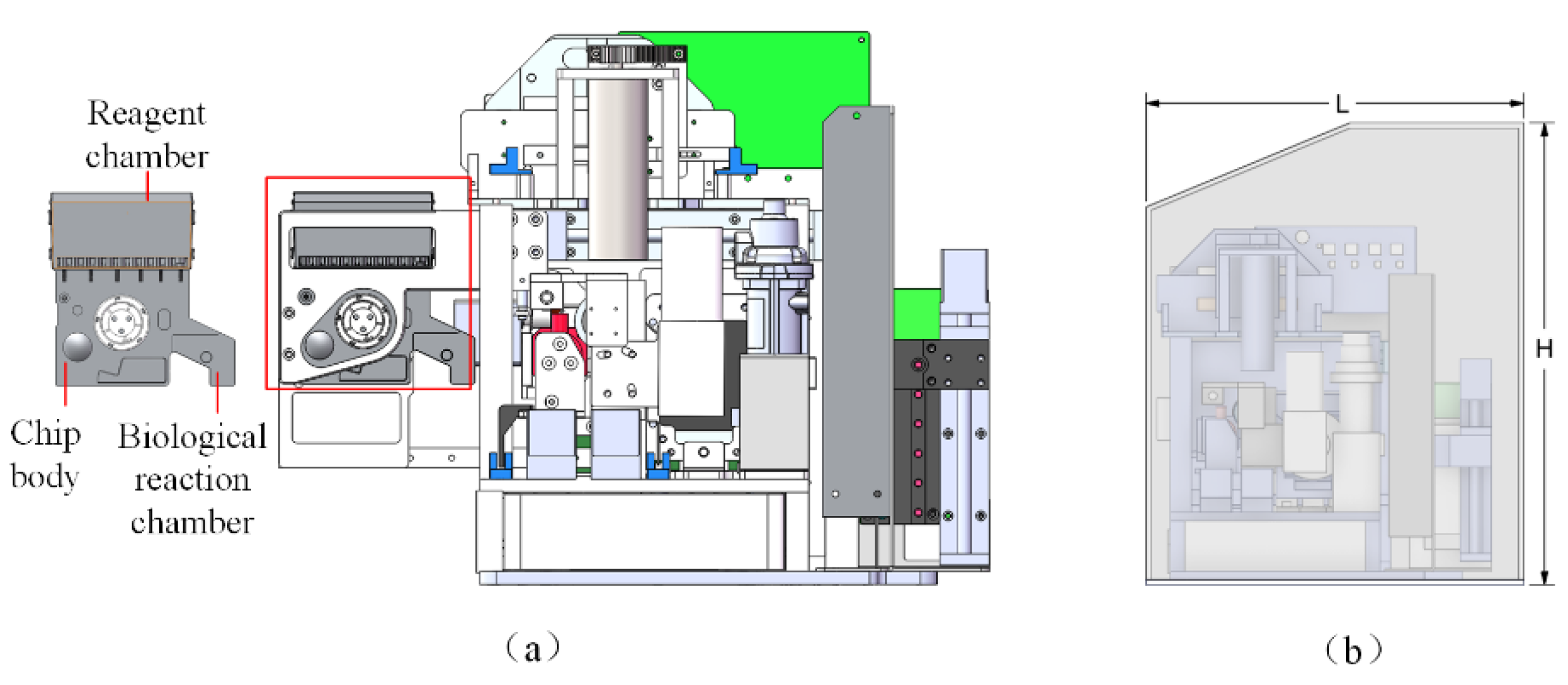
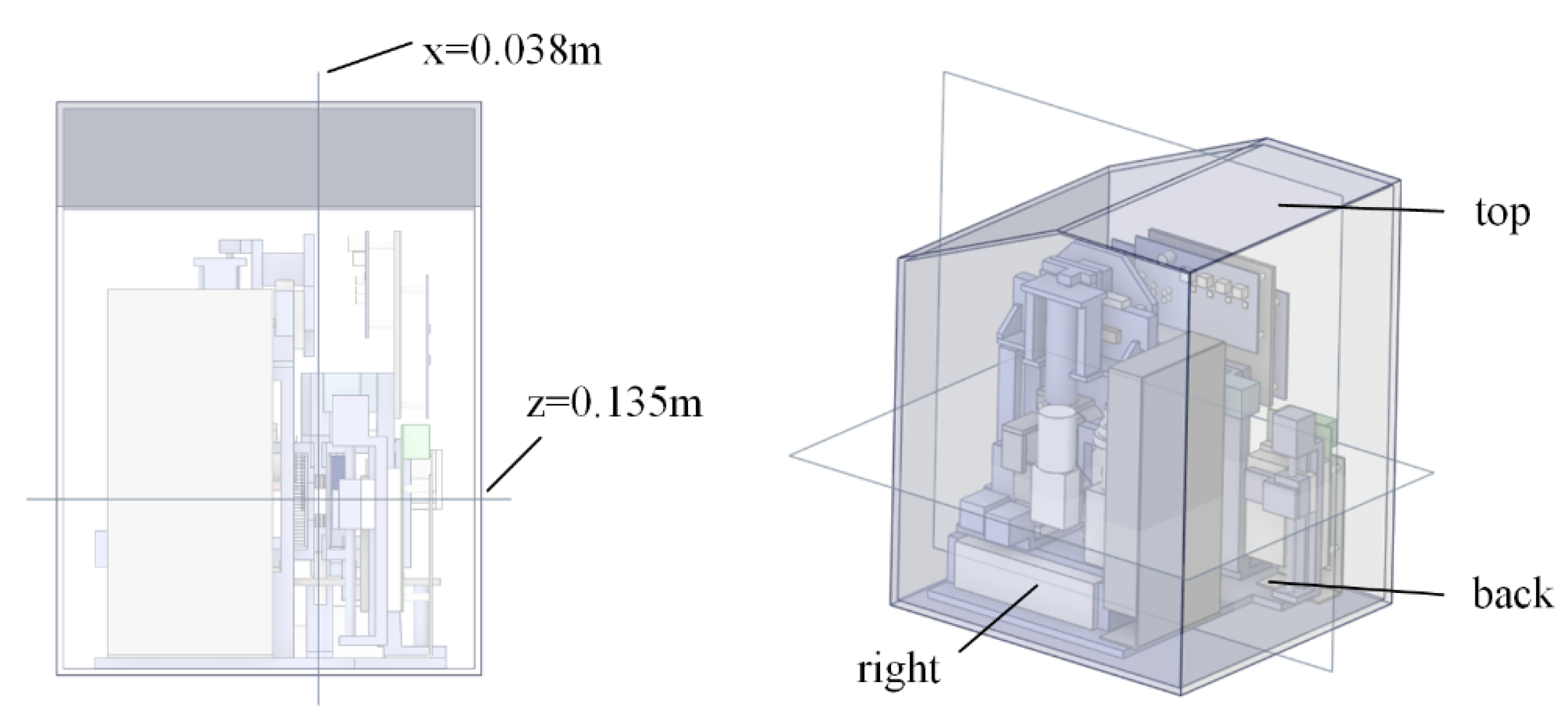
2.1. Geometry
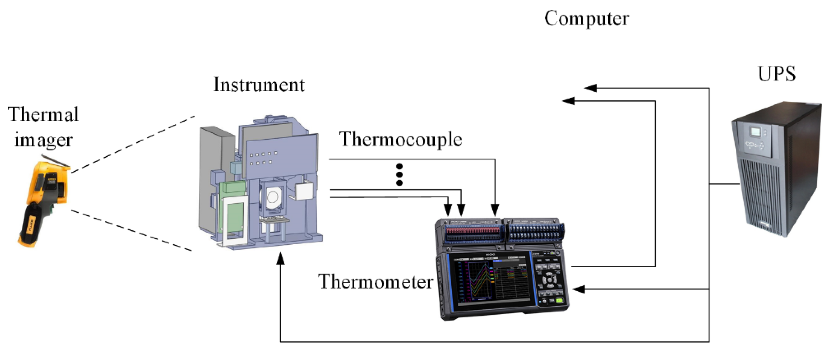
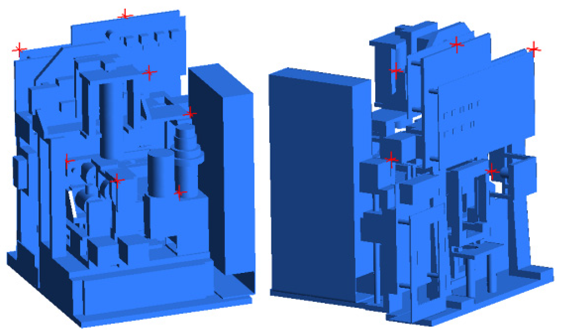
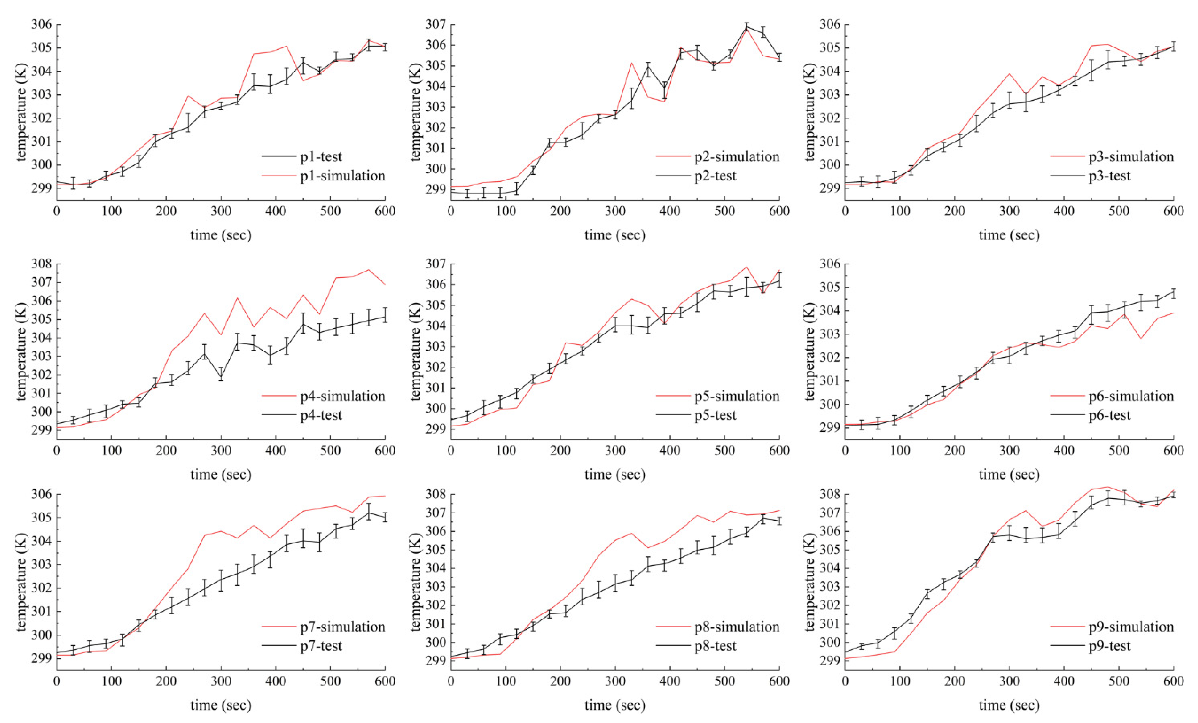
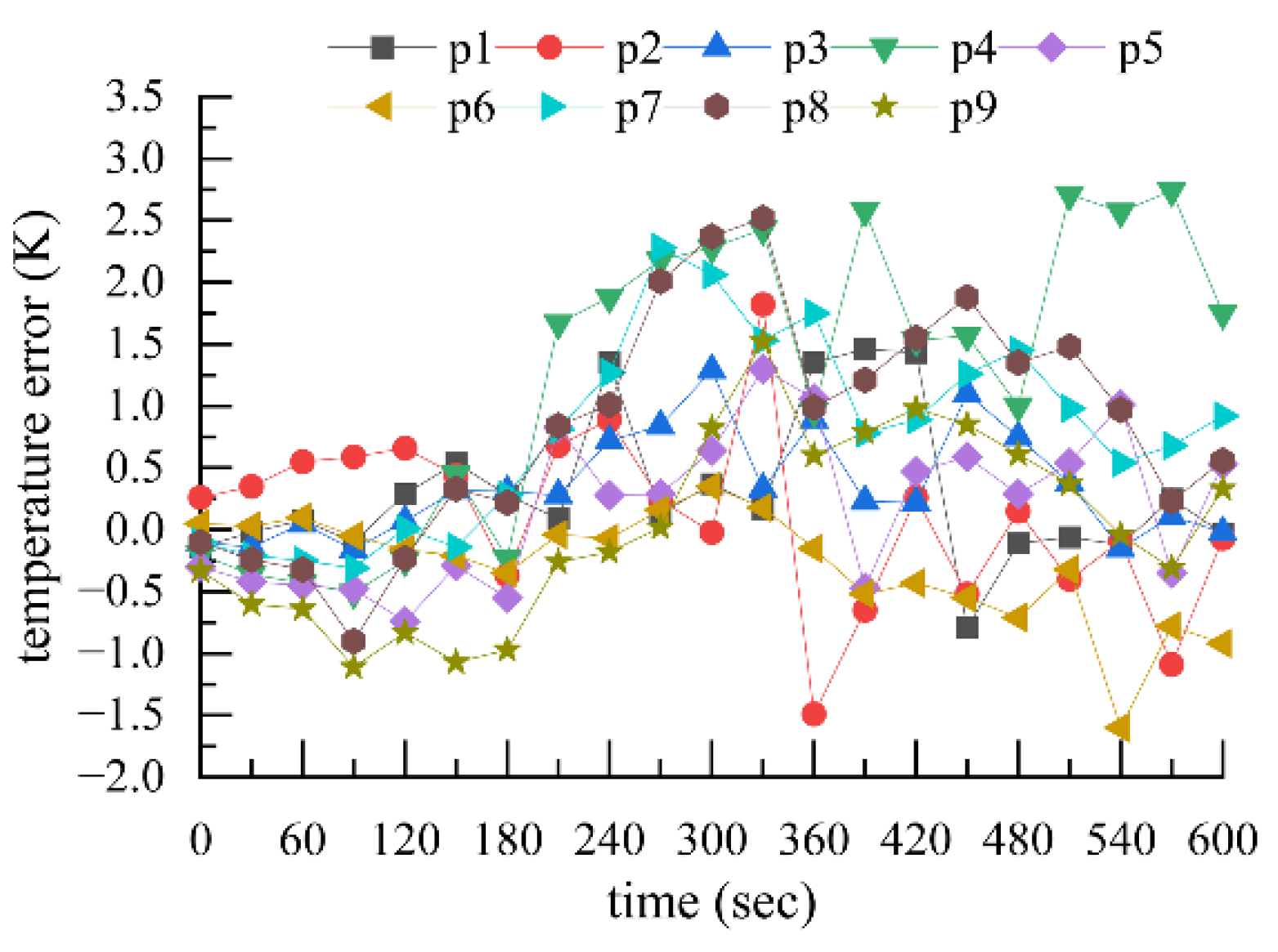
2.2. Experimental Method
3. Simulation Process
3.1. Material Parameters
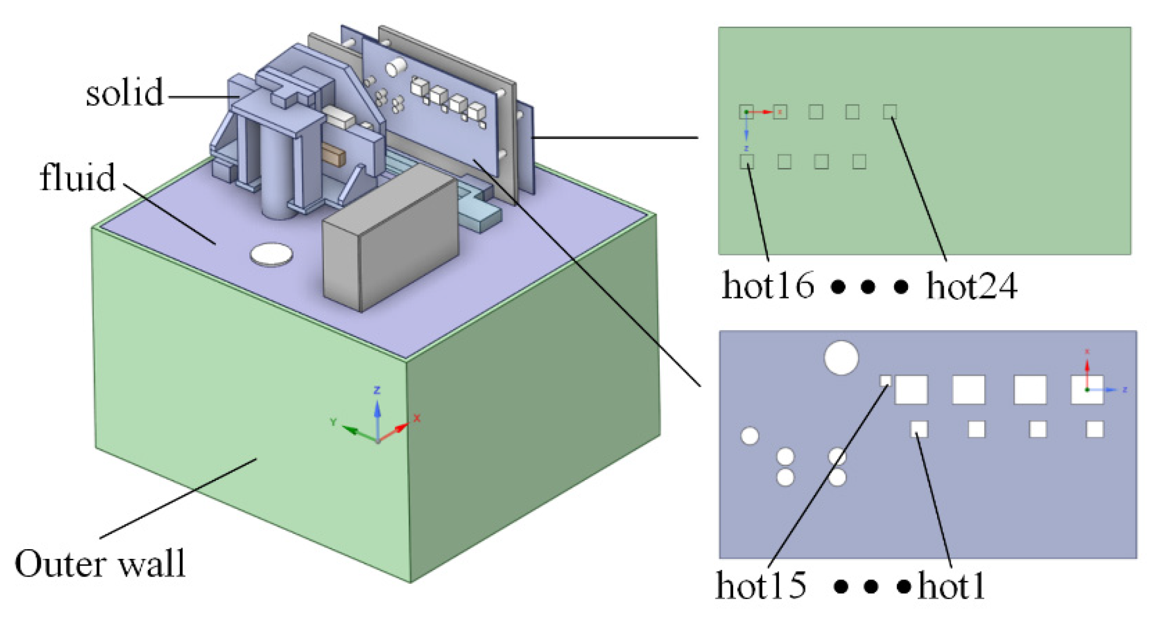
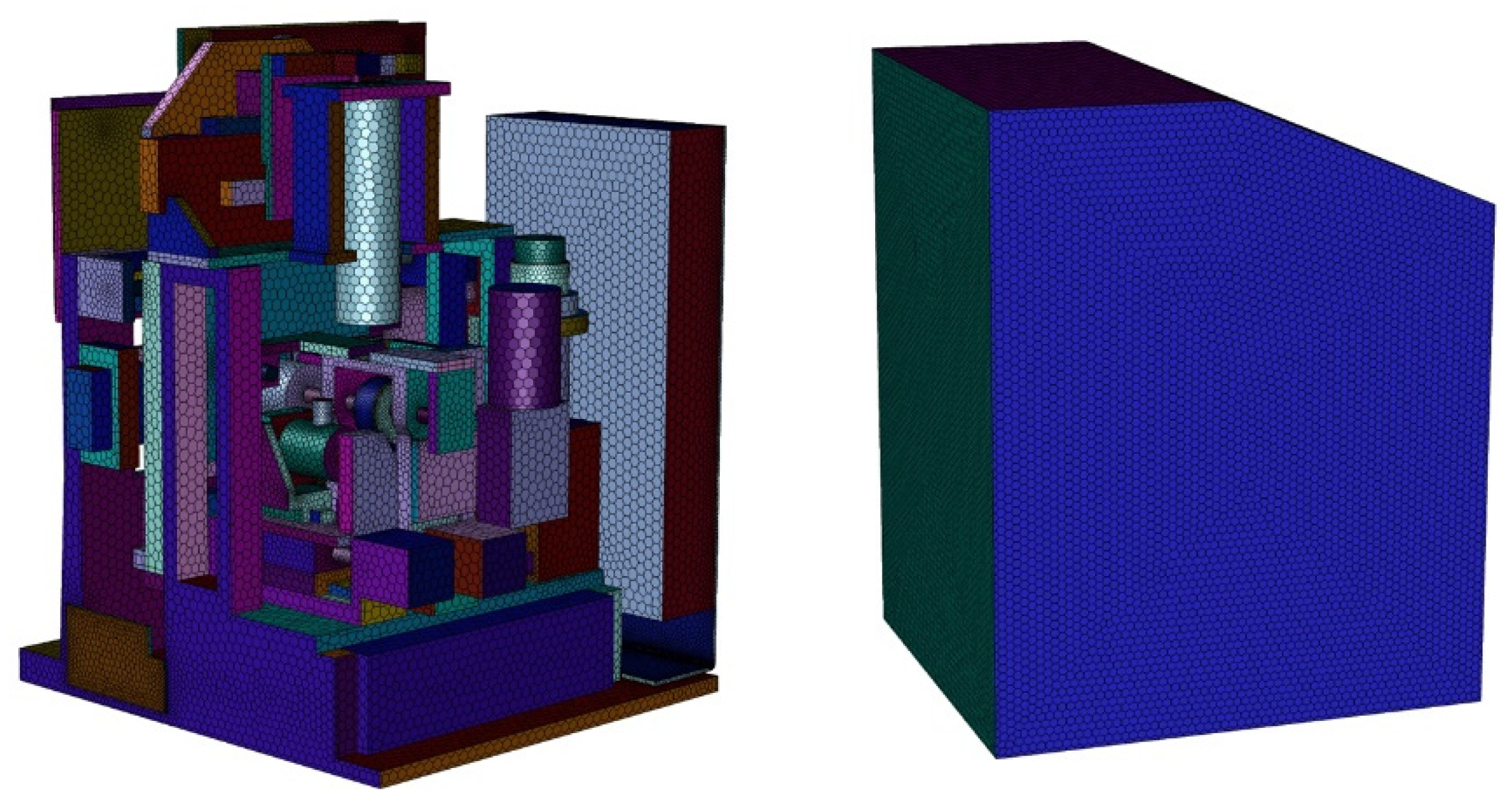
3.2. Computational Domain and Boundary Conditions
- The flow remains incompressible, ideal, and single phase.
- The initial (ambient) temperature remained constant.
- The heat lost from the enclosure to the surroundings was negligible.
- The connections between parts were considered seamless.
3.3. Grid Independence
4. Simulation Results and Discussion
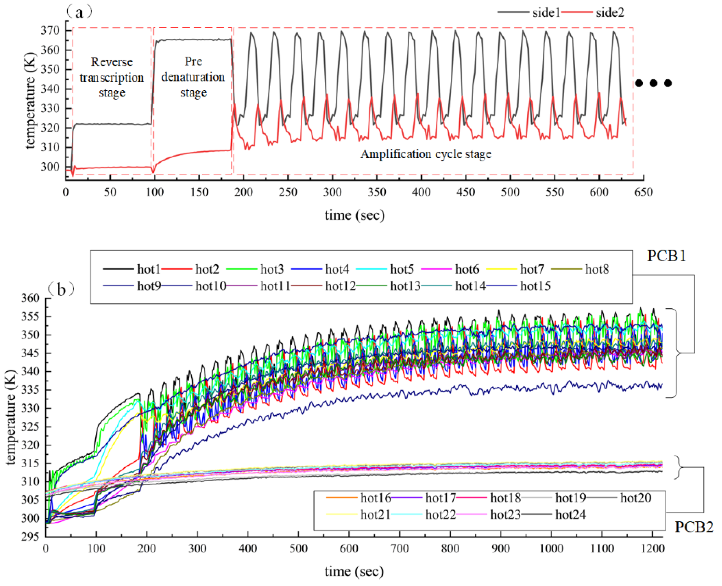
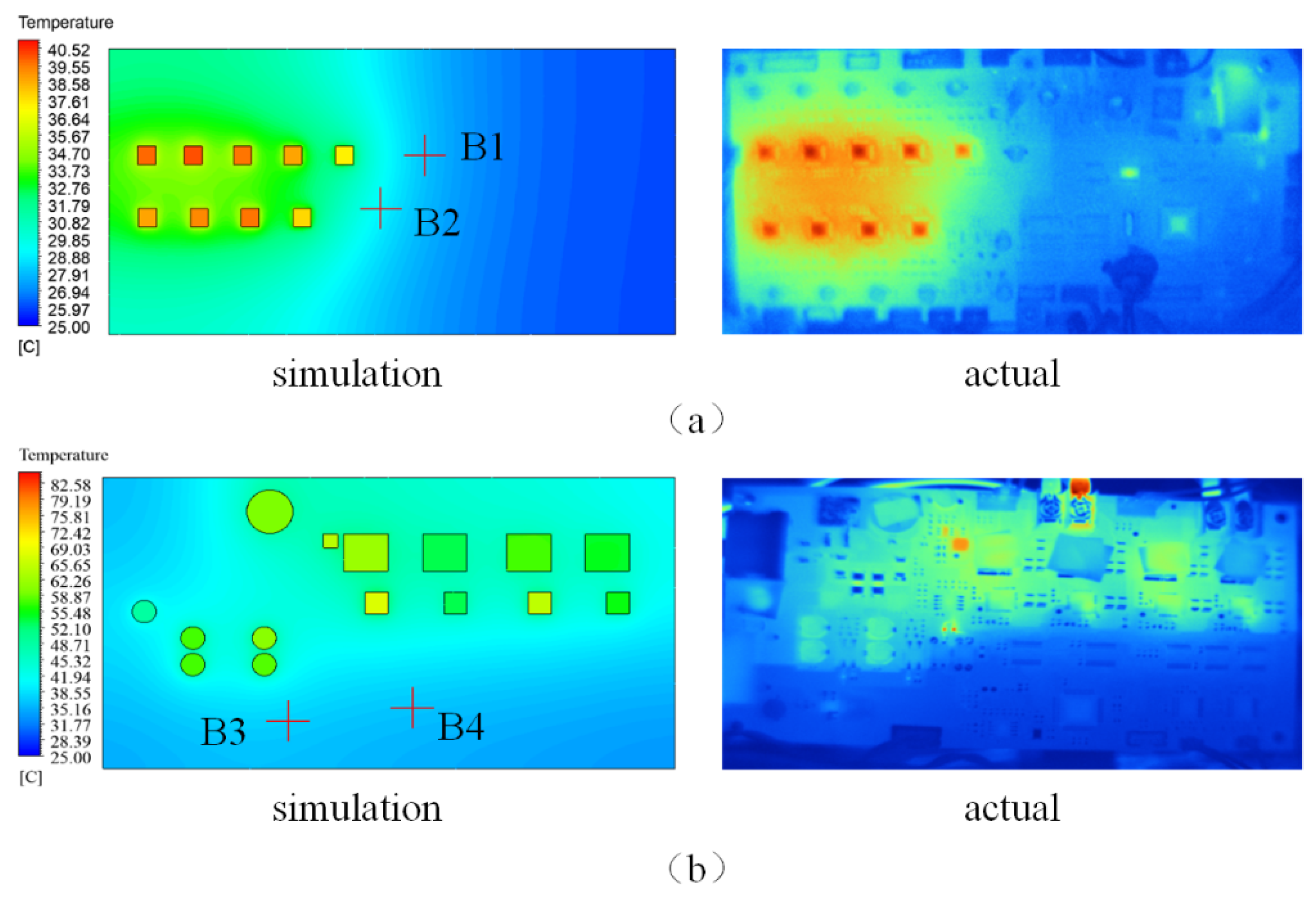
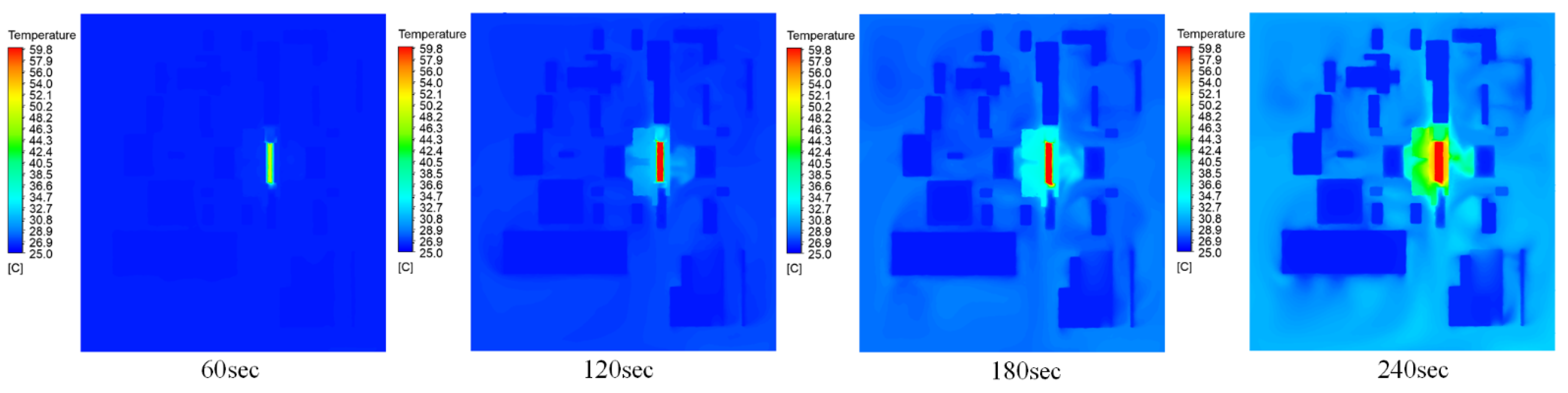
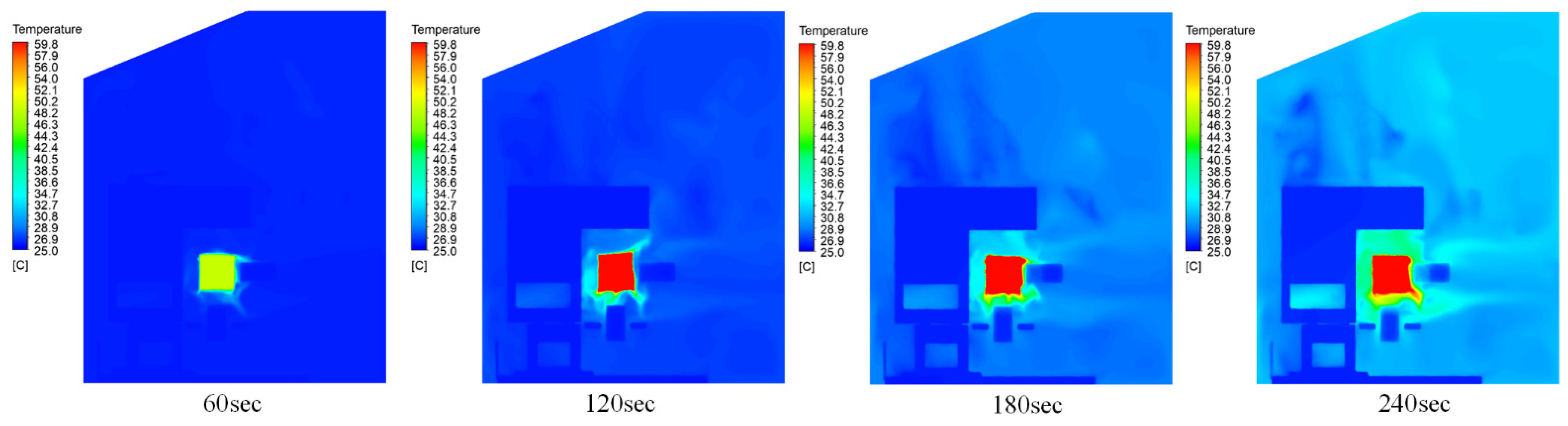
4.1. Amplification Module
4.2. PCB
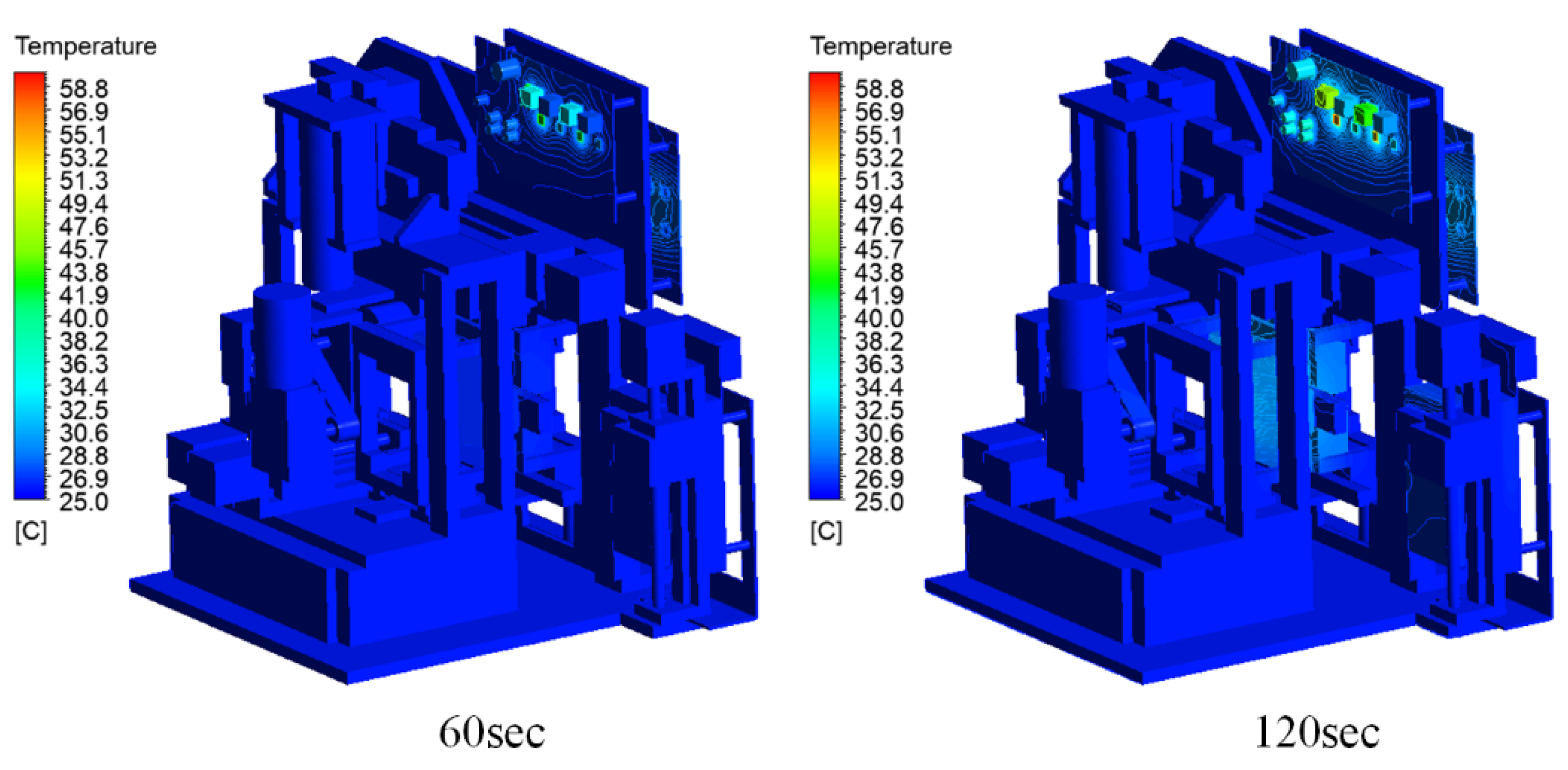
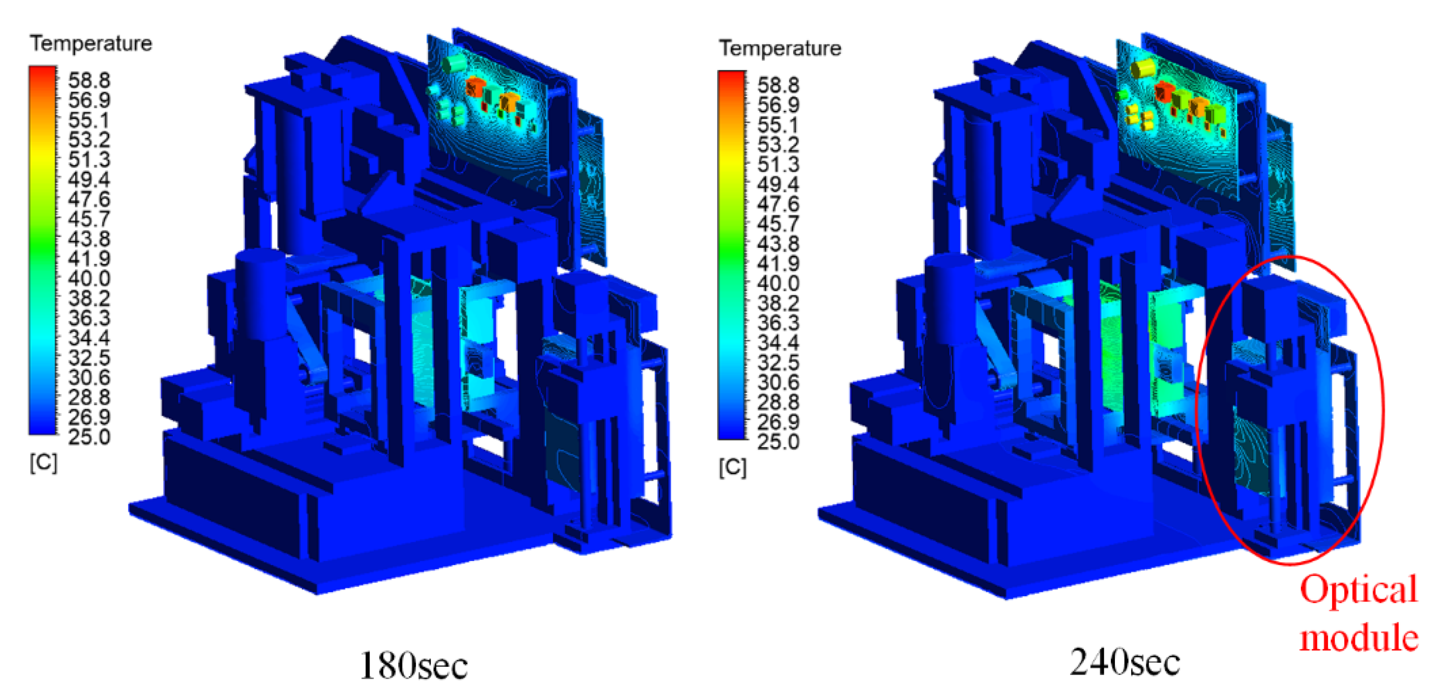
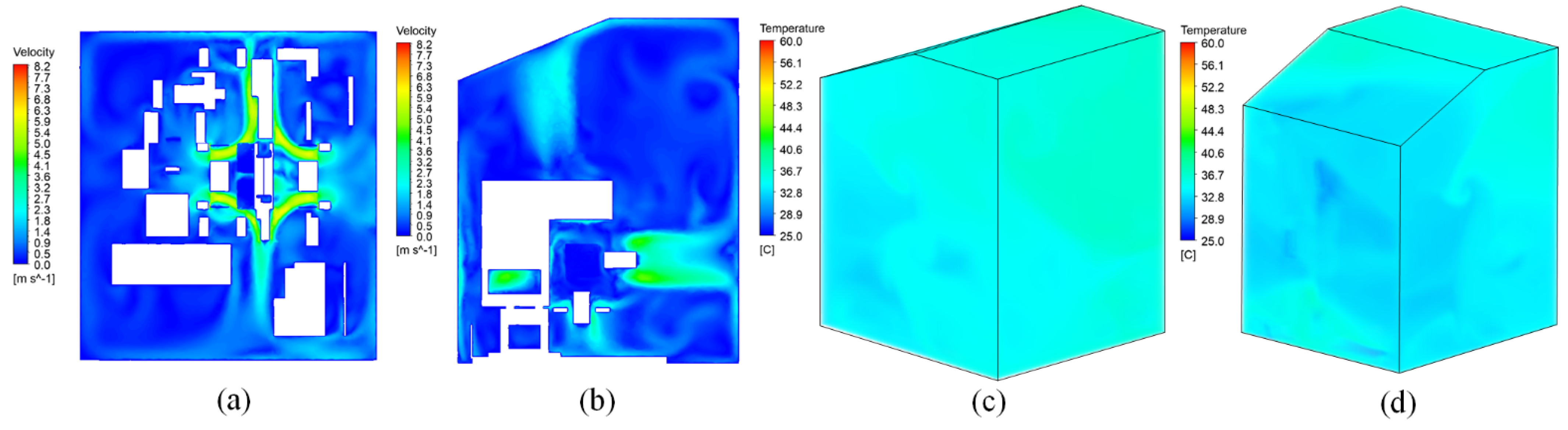
4.3. Overall Device
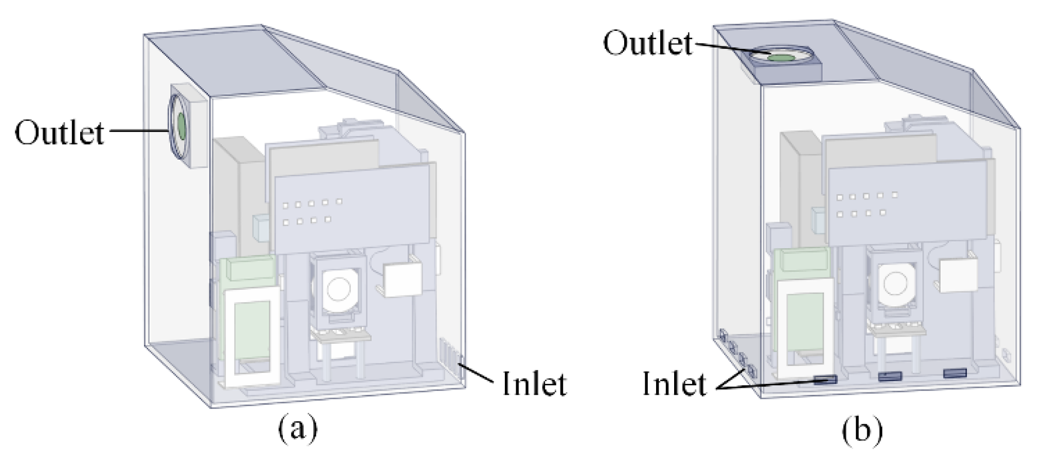
4.4. Heat-Dissipation Scheme
5. Conclusions
Author Contributions
Funding
Institutional Review Board Statement
Informed Consent Statement
Acknowledgments
Conflicts of Interest
References
- Wu, Y.; Peng, W.; Zhao, Q.; Piao, J.; Zhang, B.; Wu, X.; Wang, H.; Shi, Z.; Gong, X.; Chang, J. Immune fluorescence test strips based on quantum dots for rapid and quantitative detection of carcino-embryonic antigen. Chin. Chem. Lett. 2017, 28, 1881–1884. [Google Scholar] [CrossRef]
- Li, H.T.; Pan, J.Z.; Fang, Q. Development and Application of Digital PCR Technology. Prog. Chem. 2020, 32, 581–593. [Google Scholar]
- Mackay, I.M.; Arden, K.E.; Nitsche, A. Real-time PCR in virology. Nucleic Acids Res. 2002, 30, 1292–1305. [Google Scholar] [CrossRef] [PubMed] [Green Version]
- Valasek, M.A.; Repa, J.J. The power of real-time PCR. Adv. Physiol. Educ. 2005, 29, 151–159. [Google Scholar] [CrossRef]
- Klein, D. Quantification using real-time PCR technology: Applications and limitations. Trends Mol. Med. 2002, 8, 257–260. [Google Scholar] [CrossRef]
- Lall, P.; Pecht, M.; Hakim, E.B. Influence of Temperature on Microelectronics and System Reliability: A Physics of Failure Approach; Taylor & Francis Group: Florida, FL, USA, 1997. [Google Scholar]
- Cooper, M. Investigation of Arrhenius acceleration factor for integrated circuit early life failure region with several failure mechanisms. IEEE Trans. Compon. Packag. Technol. 2005, 28, 561–563. [Google Scholar] [CrossRef]
- Lall, P.; Pecht, M.; Hakim, E.B. Characterization of functional relationship between temperature and microelectronic reliability. Microelectron. Reliab. 1995, 35, 377–402. [Google Scholar] [CrossRef]
- Son, J.H.; Hong, S.G.; Haack, A.J.; Gustafson, L.; Song, M.S.; Hoxha, O.; Lee, L.P. Rapid Optical Cavity PCR. Adv. Healthc. Mater. 2016, 5, 167–174. [Google Scholar] [CrossRef]
- Li, J.; Liu, S.; Li, S.; Zhang, P.; Liu, H.; Shao, L. PCR Instrument Temperature Control System Based on Multimodal control. In Proceedings of the 2020 Chinese Control And Decision Conference (CCDC), Hefei, China, 22–24 August 2020; pp. 149–154. [Google Scholar] [CrossRef]
- Jalili, A.; Bagheri, M.; Shamloo, A.; Ashkezari, A.H.K. A plasmonic gold nanofilm-based microfluidic chip for rapid and inexpensive droplet-based photonic PCR. Sci. Rep. 2021, 11, 1–13. [Google Scholar] [CrossRef]
- Ramezani, A. CtNorm: Real time PCR cycle of threshold (Ct) normalization algorithm. J. Microbiol. Methods 2021, 187, 106267. [Google Scholar] [CrossRef]
- Nomada, H.; Morita, K.; Higuchi, H.; Yoshioka, H.; Oki, Y. Carbon–polydimethylsiloxane-based integratable optical technology for spectroscopic analysis. Talanta 2017, 166, 428–432. [Google Scholar] [CrossRef] [PubMed] [Green Version]
- Aziz, I.; Jamshaid, R.; Zaidiand, T.; Akhtar, I. Numerical simulation of heat transfer to optimize DNA amplification in Polymerase Chain Reaction. In Proceedings of the 2016 International Conference on Applied Mathematics, Simulation and Modelling, Beijing, China, 28–29 May 2016; pp. 456–462. [Google Scholar] [CrossRef]
- Naghdloo, A.; Ghazimirsaeed, E.; Shamloo, A. Numerical simulation of mixing and heat transfer in an integrated centrifugal microfluidic system for nested-PCR amplification and gene detection. Sens. Actuators B Chem. 2018, 283, 831–841. [Google Scholar] [CrossRef]
- Parng, S.-H.; Wu, P.-J.; Tsai, Y.-Y.; Hong, R.-S.; Lee, S.-J. A 3D tubular structure with droplet generation and temperature control for DNA amplification. Microfluid. Nanofluidics 2021, 25, 1–8. [Google Scholar] [CrossRef]
- Zhou, A.; Liu, B.; Xu, X.; Li, W. An Analysis of the Two-Dimensional Heat Transfer Model of the PCR Instrument Pedestal. In Proceedings of the An Analysis of the Two-Dimensional Heat Transfer Model of the PCR Instrument Pedestal, Shanghai, China, 28–29 May 2016. [Google Scholar] [CrossRef] [Green Version]
- Raza, M.; Malik, I.R.; Akhtar, I. Design and Thermal Analysis of Sample Block PCR for DNA Amplification. In Proceedings of the 2020 17th International Bhurban Conference on Applied Sciences and Technology, Islamabad, Pakistan, 14–18 January 2020; pp. 210–217. [Google Scholar]
- Hao, H.; Guan, X.; Chen, J.; Pan, Z. Internal cooling design of PCB based on thermal model. Electronic Compon. Mater. 2016, 35, 76–79. [Google Scholar]
- Mesforush, S.; Jahanshahi, A.; Zadeh, M.K. Finite element simulation of isothermal regions in serpentine shaped PCB electrodes of a micro-PCR device. In Proceedings of the 2019 27th Iranian Conference on Electrical Engineering, Yazd, Iran, 30 April 2019–2 May 2019; pp. 280–284. [Google Scholar] [CrossRef]
- Fedorov, A.G.; Viskanta, R. Three-dimensional conjugate heat transfer in the microchannel heat sink for electronic packaging. Int. J. Heat Mass Transf. 2000, 43, 399–415. [Google Scholar] [CrossRef]
- Shankaran, G.V.; Singh, R.K. Selection of Appopriate Thermal Model For Printed Circut Boards in CFD Analysis. In Proceedings of the thermal and Thermomechanical Proceedings 10th Intersociety Conference on Phenomena in Electronics Systems, San Diego, CA, USA, 30 May–2 June 2006; pp. 234–242. [Google Scholar]
- Jun, Y.; Dakui, F.; Hang, Z. Numerical simulation of pump jet propulsor and analysis of scale effect. Shipbuild. China 2020, 61, 91–99. [Google Scholar]
- Versteeg, H.K.; Malalasekera, W. An Introduction to Computational Fluid Dynamics: The Finite Volume Method; Pearson Education: New York, NY, USA, 2007. [Google Scholar]
- Behera, R.C.; Dutta, P.; Srinivasan, K. Numerical Study of Interrupted Impinging Jets for Cooling of Electronics. IEEE Trans. Compon. Packag. Technol. 2007, 30, 275–284. [Google Scholar] [CrossRef] [Green Version]
- Boulet, M.; Marcos, B.; Dostie, M.; Moresoli, C. CFD modeling of heat transfer and flow field in a bakery pilot oven. J. Food Eng. 2010, 97, 393–402. [Google Scholar] [CrossRef]
- Jo, J.C.; Kang, D.G. CFD analysis of thermally stratified flow and conjugate heat transfer in a PWR pressurizer surgeline. J. Press. Vessel. Technol. 2010, 132, 021301. [Google Scholar] [CrossRef]
- Widiawaty, C.D.; Siswantara, A.I.; Budiarso; Gunadi, G.G.R.; Pujowidodo, H.; Syafei, M.H.G. A CFD simulation and experimental study: Predicting heat transfer performance using SST k-ω turbulence model. IOP Conf. Ser. Mater. Sci. Eng. 2020, 909, 012004. [Google Scholar] [CrossRef]
- Han, J.W.; Zhao, C.J.; Yang, X.T.; Qian, J.P.; Fan, B.L. Computational modeling of airflow and heat transfer in a vented box during cooling: Optimal package design. Appl. Therm. Eng. 2015, 91, 883–893. [Google Scholar] [CrossRef]
- Menter, F.R. Two-equation eddy-viscosity turbulence models for engineering applications. AIAA J. 1994, 32, 1598–1605. [Google Scholar] [CrossRef] [Green Version]
- Menter, F.R.; Kuntz, M.; Langtry, R. Ten years of industrial experience with the SST turbulence model. Turbul. Heat Mass Transf. 2003, 4, 625–632. [Google Scholar]
- Wilcox, D.C. Turbulence Modeling for CFD; DCW industries: La Canada, CA, USA, 1998. [Google Scholar]
- Król, A.; Król, M. Study on numerical modeling of jet fans. Tunn. Undergr. Space Technol. 2018, 73, 222–235. [Google Scholar] [CrossRef]
- Fan, J.; Dong, H.; Xu, X.; Teng, D.; Yan, B.; Zhao, Y. Numerical Investigation on the Influence of Mechanical Draft Wet-Cooling Towers on the Cooling Performance of Air-Cooled Condenser with Complex Building Environment. Energies 2019, 12, 4560. [Google Scholar] [CrossRef] [Green Version]
- Paramanandam, K.; Venkatachalapathy, S.; Srinivasan, B. Heat transfer enhancement in microchannels using ribs and secondary flows. Int. J. Numer. Methods Heat Fluid Flow 2021, 32, 2299–2319. [Google Scholar] [CrossRef]
- Luo, H.; Lu, B.; Zhang, J.; Wu, H.; Wang, W. A grid-independent EMMS/bubbling drag model for bubbling and turbulent fluidization. Chem. Eng. J. 2017, 326, 47–57. [Google Scholar] [CrossRef] [Green Version]
- Zaidan, M.H.; Alkumait, A.A.; Ibrahim, T.K. Assessment of heat transfer and fluid flow characteristics within finned flat tube. Case Stud. Therm. Eng. 2018, 12, 557–562. [Google Scholar] [CrossRef]


| (m) | (m2) | (m2) | (m2) | (m2) | |
|---|---|---|---|---|---|
| PCB1 | 0.0016 | 0.012 | 0.012 | 0.012 | 0.01 |
| PCB2 | 0.0016 | 0.023 | 0.02 | 0.022 | 0.019 |
| (m) | (m) | (m2) | (W·m−1·K−1) | (W·m−1·K−1) | N | |
|---|---|---|---|---|---|---|
| PCB1 | 0.000035 | 0.0000487 | 0.013 | 388 | 0.35 | 4 |
| PCB2 | 0.000035 | 0.0000487 | 0.024 | 388 | 0.35 | 4 |
| Material | Density (kg·m−3) | Specific Heat (J·kg−1·K−1) | Thermal Conductivity (W·m−1·K−1) |
|---|---|---|---|
| 6061 aluminum alloy | 2750 | 896 | 155 |
| Stainless steel | 8055 | 480 | 13.8 |
| Packaging plastic | 2090 | 900 | 0.67 |
| FR4 | 1900 | 1369 | 0.3 |
| Pom | 1430 | 1.465 | 0.23 |
| Si | 2329 | 700 | 130 |
| Ceramics | 1345 | 710 | 150 |
| Acrylic | 1190 | 1464 | 0.18 |
| Red copper | 8960 | 385 | 401 |
| Wood | 700 | 2310 | 0.173 |
| Object | Type |
|---|---|
| Fluid and solid contact surfaces | couple wall |
| Fan boundary | polynomial |
| TEC side1 and side2 | temperature wall |
| Heat source on the PCB | values |
| Fluid | air, incompressible |
| Inlet and outlet | pressure inlet/outlet |
| Pressure–velocity couple | simple |
| The discretization of convection–diffusion | second-order upwind |
Publisher’s Note: MDPI stays neutral with regard to jurisdictional claims in published maps and institutional affiliations. |
© 2022 by the authors. Licensee MDPI, Basel, Switzerland. This article is an open access article distributed under the terms and conditions of the Creative Commons Attribution (CC BY) license (https://creativecommons.org/licenses/by/4.0/).
Share and Cite
Lin, X.; Cai, W.; Huang, S.; Zhu, S.; Zhang, D. Conjugate Heat Transfer Analysis and Heat Dissipation Design of Nucleic Acid Detector Instrument. Appl. Sci. 2022, 12, 11966. https://doi.org/10.3390/app122311966
Lin X, Cai W, Huang S, Zhu S, Zhang D. Conjugate Heat Transfer Analysis and Heat Dissipation Design of Nucleic Acid Detector Instrument. Applied Sciences. 2022; 12(23):11966. https://doi.org/10.3390/app122311966
Chicago/Turabian StyleLin, Xiaohui, Weihuang Cai, Shaolei Huang, Sijie Zhu, and Dongxu Zhang. 2022. "Conjugate Heat Transfer Analysis and Heat Dissipation Design of Nucleic Acid Detector Instrument" Applied Sciences 12, no. 23: 11966. https://doi.org/10.3390/app122311966
APA StyleLin, X., Cai, W., Huang, S., Zhu, S., & Zhang, D. (2022). Conjugate Heat Transfer Analysis and Heat Dissipation Design of Nucleic Acid Detector Instrument. Applied Sciences, 12(23), 11966. https://doi.org/10.3390/app122311966