
Comparative Analysis of Viscous Damping Model and Hysteretic Damping Model


Abstract
:1. Introduction
2. Comparative Analysis of Transient Responses Based on Different Damping Models
2.1. The Transient Response of Viscous Damped System
2.2. The Transient Response of Hysteretic Damped System
2.3. Comparative Analysis of the Transient Response
3. Comparative Analysis of Steady Responses Based on Different Damping Models
3.1. The Steady Response of Viscous Damped System
3.2. The Steady Response of Hysteretic Damped System
3.3. Comparative Analysis of the Steady Response
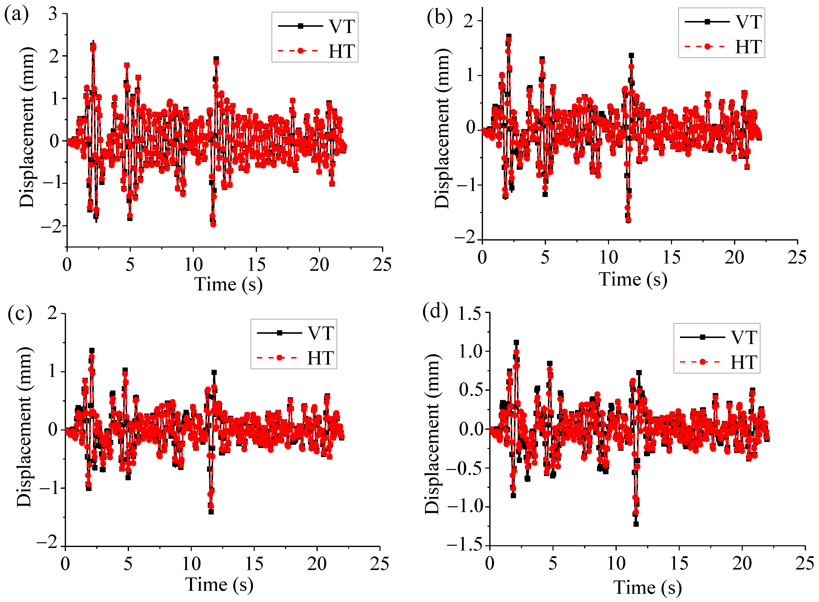
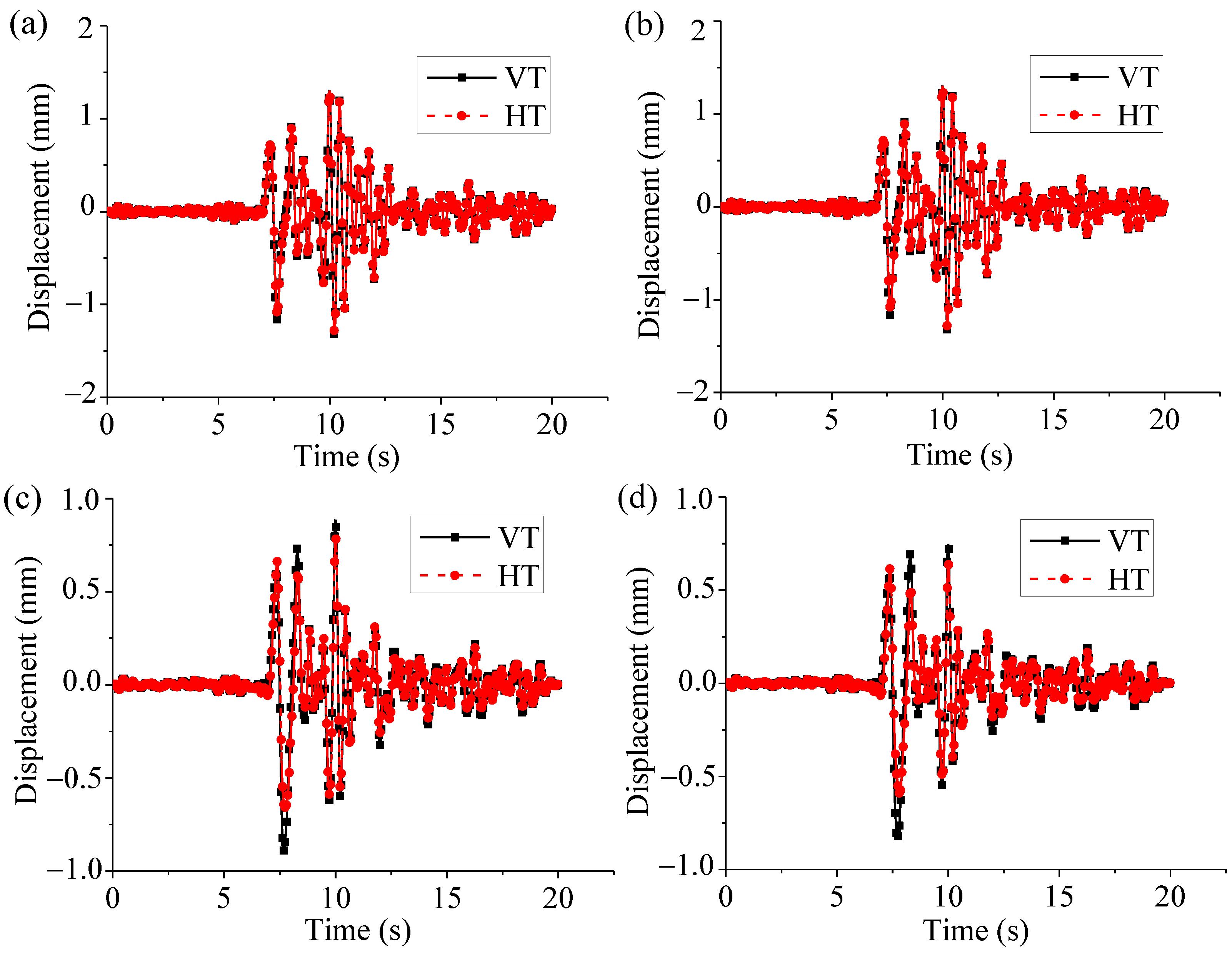
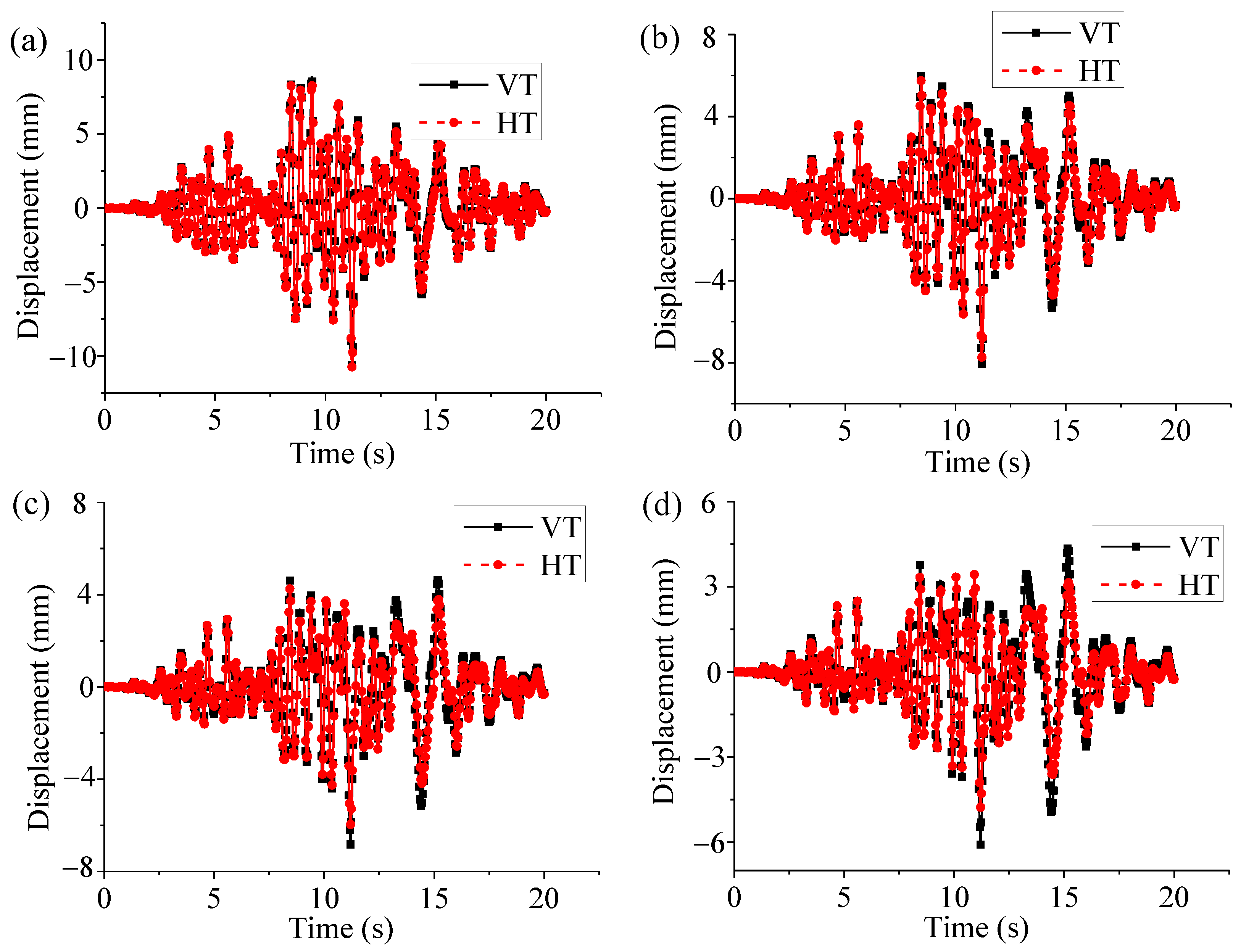
4. Numerical Examples
5. Conclusions
- (1)
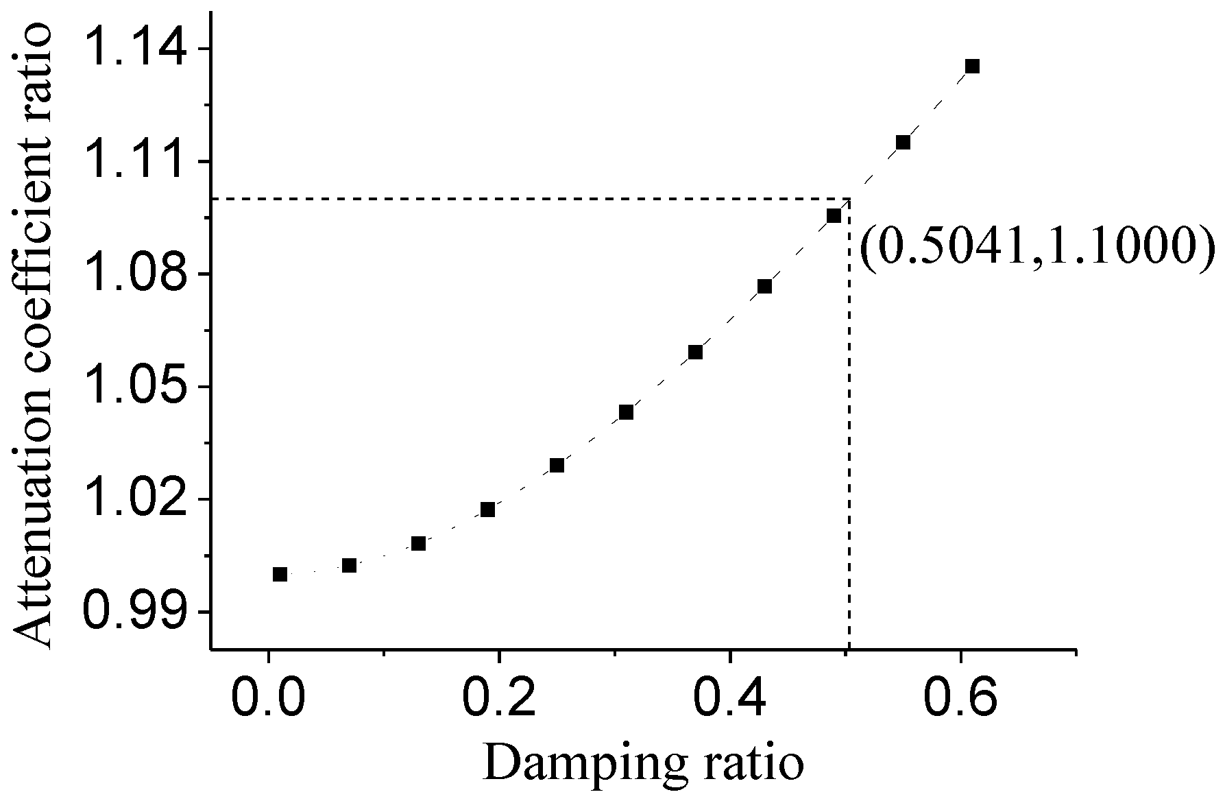
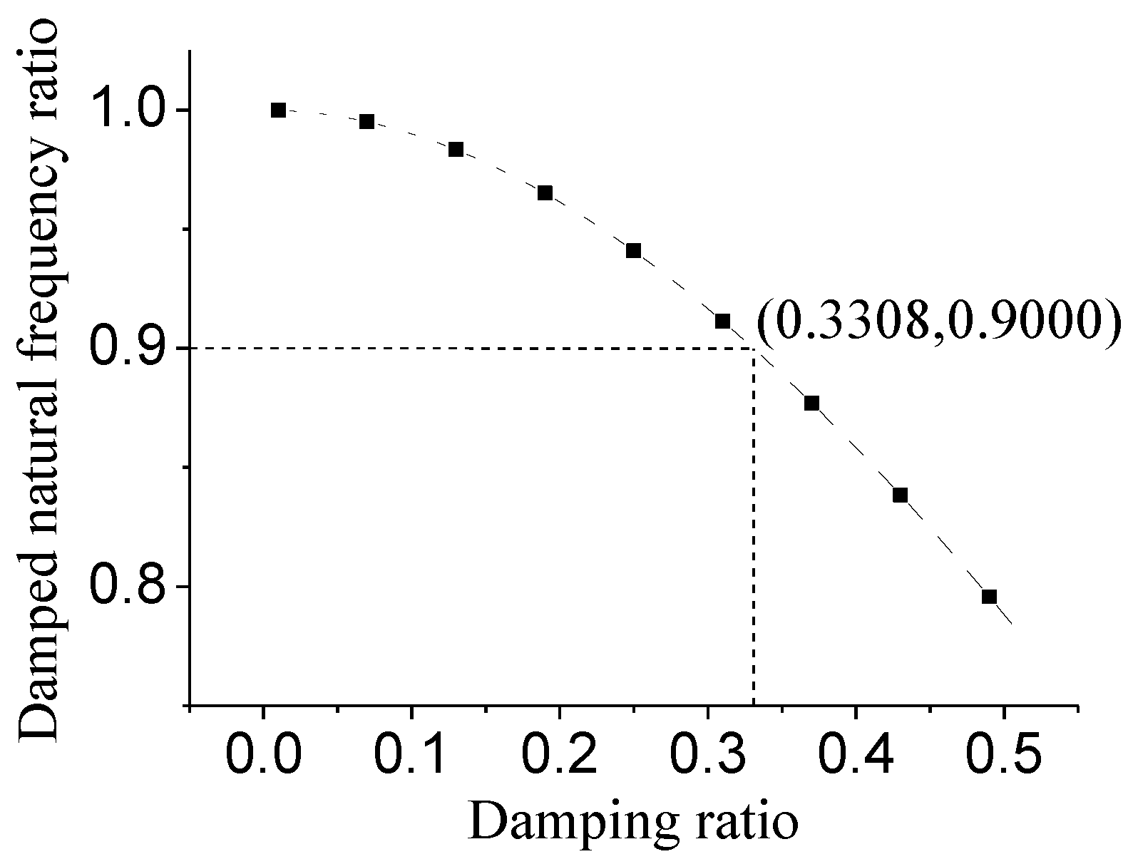
- The attenuation coefficient and damped natural frequency are important parameters of the transient response. When the relative error of the attenuation coefficients for the two damping models was less than 10%, the damping ratio was less than 0.5041. When the relative error of damped natural frequencies for the two damping models was less than 10%, the damping ratio is less than 0.3308.
- (2)
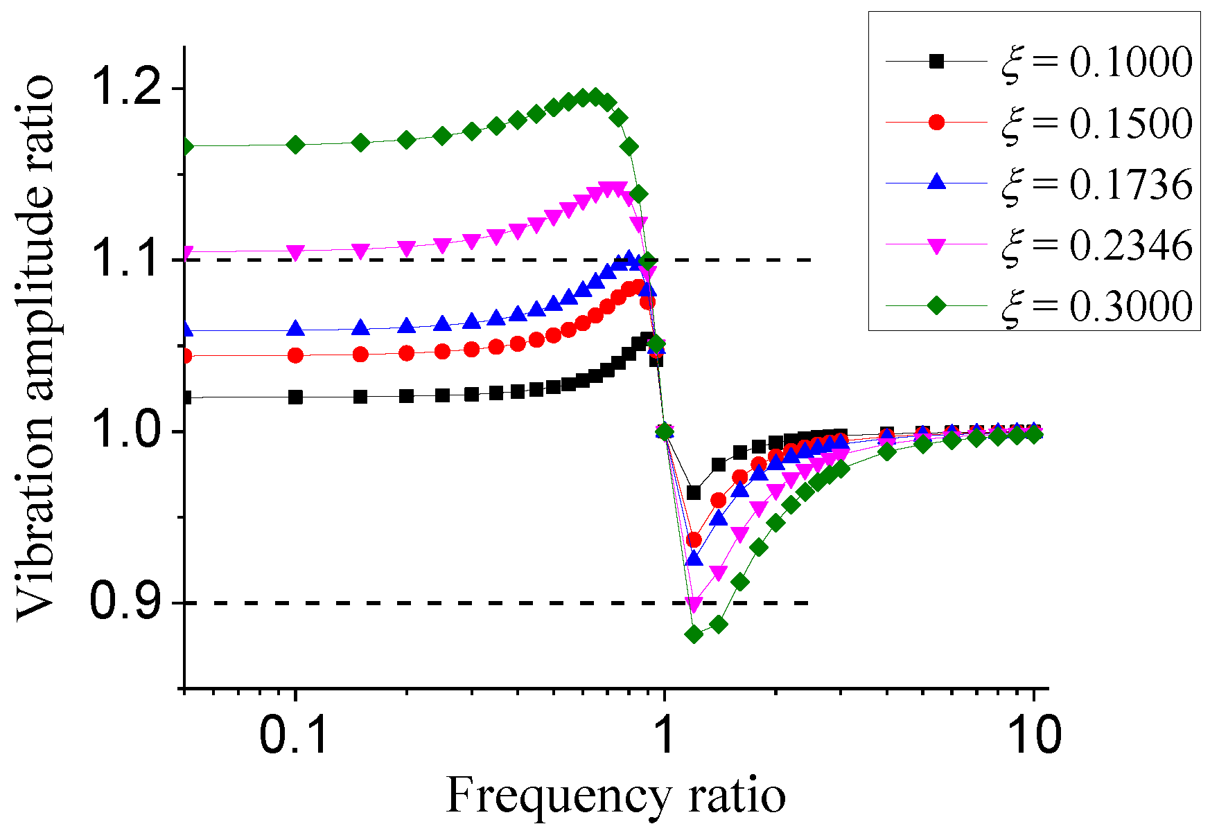
- Earthquake waves can be decomposed into a series of harmonic waves. The vibration amplitude of the steady response is an important parameter. When the relative error of the maximum and minimum values of the vibration amplitude ratio for the two damping models was less than 10%, the damping ratio was less than 0.1736.
- (3)
- The numerical examples show that with the increase in damping ratio, the difference between the dynamic responses calculated by the two damping models gradually increases. Based on the comparative analysis of the transient and steady responses, the threshold of the damping ratio was selected as 0.1736, conservatively. When the damping ratio was less than 0.1736, the dynamic responses of the two damping models were approximately equal.
Author Contributions
Funding
Institutional Review Board Statement
Informed Consent Statement
Data Availability Statement
Conflicts of Interest
References
- Dowell, E. Modal damping in a finite element model (L). J. Acoust. Soc. Am. 2016, 140, 2288–2289. [Google Scholar] [CrossRef]
- Sun, Q.; Zhang, K.; Ju, J. Parameter identification of general damping model based on structural dynamic response. J. Phys. Conf. Ser. 2021, 1885, 52051. [Google Scholar] [CrossRef]
- Cooley, C.G.; Tran, T.Q.; Chai, T. Comparison of viscous and structural damping models for piezoelectric vibration energy harvesters. Mech. Syst. Signal Process. 2018, 110, 130–138. [Google Scholar] [CrossRef]
- Clough, R.W.; Penzien, J. Dynamics of Structures; McGraw-Hill: New York, NY, USA, 1993. [Google Scholar]
- Roderic, L. Viscoelastic Materials; Cambridge University Press: Cambridge, UK, 2009. [Google Scholar]
- Zhao, C.; Wang, P.; Yi, Q.; Sheng, X.; Lu, J. A detailed experimental study of the validity and applicability of slotted stand-off layer rail dampers in reducing railway vibration and noise. J. Low Freq. Noise Vib. Act. Control 2018, 37, 896–910. [Google Scholar] [CrossRef] [Green Version]
- Zhou, Y.; Shi, F.; Ozbulut, O.E.; Xu, H.; Zi, D. Experimental characterization and analytical modeling of a large-capacity high-damping rubber damper. Struct. Control Health 2018, 25, e2183. [Google Scholar] [CrossRef]
- Adhikari, S.; Woodhouse, J. Identification of damping: Part 1, viscous damping. J. Sound Vib. 2001, 243, 43–61. [Google Scholar] [CrossRef] [Green Version]
- Orzechowski, G.; Escalona, J.L.; Dmitrochenko, O.; Mohammadi, N.; Mikkola, A.M. Modeling viscous damping for transverse oscillations in reeving systems using the Arbitrary Lagrangian-Eulerian Modal approach. J. Sound Vib. 2022, 534, 117009. [Google Scholar] [CrossRef]
- Feng, Z.; Gong, J. Effect of Viscous Damping Models on Displacement Ductility Demands for SDOF Systems. KSCE J. Civ. Eng. 2021, 25, 4698–4709. [Google Scholar] [CrossRef]
- Sun, P.; Yang, H.; Kang, L. Time-domain analysis for dynamic responses of non-classically damped composite structures. Compos. Struct. 2020, 251, 112554. [Google Scholar] [CrossRef]
- Papageorgiou, A.V.; Gantes, C.J. Equivalent uniform damping ratios for linear irregularly damped concrete/steel mixed structures. Soil Dyn. Earthq. Eng. 2011, 31, 418–430. [Google Scholar] [CrossRef]
- Pan, D.; Chen, G.; Wang, Z. Suboptimal Rayleigh damping coefficients in seismic analysis of viscously-damped structures. Earthq. Eng. Eng. Vib. 2014, 13, 653–670. [Google Scholar] [CrossRef]
- Yang, F.; Zhi, X.; Fan, F. Effect of complex damping on seismic responses of a reticulated dome and shaking table test validation. Thin-Walled Struct. 2019, 134, 407–418. [Google Scholar] [CrossRef]
- Reggio, A.; De Angelis, M. Modelling and identification of structures with rate-independent linear damping. Meccanica 2015, 50, 617–632. [Google Scholar] [CrossRef]
- Vaiana, N.; Sessa, S.; Marmo, F.; Rosati, L. A class of uniaxial phenomenological models for simulating hysteretic phenomena in rate-independent mechanical systems and materials. Nonlinear Dyn. 2018, 93, 1647–1669. [Google Scholar] [CrossRef]
- Vaiana, N.; Sessa, S.; Rosati, L. A generalized class of uniaxial rate-independent models for simulating asymmetric mechanical hysteresis phenomena. Mech. Syst. Signal Process. 2021, 146, 106984. [Google Scholar] [CrossRef]
- Bert, C.W. Material damping: An introductory review of mathematical models, measures and experimental techniques. J. Sound Vib. 1973, 29, 129–153. [Google Scholar] [CrossRef]
- Pan, D.; Fu, X.; Qi, W. The direct integration method with virtual initial conditions on the free and forced vibration of a system with hysteretic damping. Appl. Sci. 2019, 9, 3707. [Google Scholar] [CrossRef] [Green Version]
- Theodorsen, T.; Garrick, I.E. Mechanism of Flutter: A Theoretical and Experimental Investigation of the Flutter Problem; National Advisory Committee for Aeronautics: Washington, DC, USA, 1940. [Google Scholar]
- Inaudi, J.A.; Kelly, J. Linear hysteretic damping and the Hilbert transform. J. Eng. Mech. 1995, 121, 626–632. [Google Scholar] [CrossRef]
- Sun, P.; Yang, H.; Deng, Y. Complex mode superposition method of nonproportionally damped linear systems with hysteretic damping. J. Vib. Control 2021, 27, 1453–1465. [Google Scholar] [CrossRef]
- Nakamura, N. Practical causal hysteretic damping. Earthq. Eng. Struct. Dyn. 2007, 36, 597–617. [Google Scholar] [CrossRef]
- Parker, K.J. Real and causal hysteresis elements. J. Acoust. Soc. Am. 2014, 135, 3381–3389. [Google Scholar] [CrossRef] [PubMed] [Green Version]
- Tsai, H.; Kelly, J.M. Dynamic parameter identification for non-linear isolation systems in response spectrum analysis. Earthq. Eng. Struct. Dyn. 1989, 18, 1119–1132. [Google Scholar] [CrossRef]
- Chopra, A.K. Dynamics of Structures: Theory and Applications to Earthquake Engineering, 3rd ed.; Prentice-Hall: Englewood Cliffs, NJ, USA, 2007. [Google Scholar]
- Vaiana, N.; Rosati, L. Classification and unified phenomenological modeling of complex uniaxial rate-independent hysteretic responses. Mech. Syst. Signal Process. 2023, 182, 109539. [Google Scholar] [CrossRef]
- Lin, R.M.; Zhu, J. On the relationship between viscous and hysteretic damping models and the importance of correct interpretation for system identification. J. Sound Vib. 2009, 325, 14–33. [Google Scholar] [CrossRef]
- Bilbao, A.; Avilés, R.; Agirrebeitia, J.; Ajuria, G. Proportional damping approximation for structures with added viscoelastic dampers. Finite Elem. Anal. Des. 2006, 42, 492–502. [Google Scholar] [CrossRef]


| Earthquake Name | Time (s) | Peak Ground Acceleration (g) | Dominant Frequency (Rad/s) |
|---|---|---|---|
| El Centro | 22 | 0.0051 | 14.8796 |
| Tianjin | 20 | 0.0102 | 7.0563 |
| Chi-Chi | 20 | 0.0204 | 4.1417 |
| Category | El Centro Wave | Tianjin Wave | Chichi Wave | |||
|---|---|---|---|---|---|---|
| VT | HT | VT | HT | VT | HT | |
| Peek displacement (mm) | 2.3749 | 2.3368 | 1.3369 | 1.3124 | 10.6377 | 10.7779 |
| Relative error (%) | — | 1.60 | — | 1.83 | — | 1.32 |
| Peek velocity (mm/s) | 28.1130 | 27.3384 | 19.1281 | 19.1565 | 133.0985 | 133.3709 |
| Relative error (%) | — | 2.76 | — | 0.15 | — | 0.20 |
| Peek acceleration (mm/s2) | 457.7155 | 449.7389 | 261.4425 | 261.8755 | 2197.0835 | 2144.0104 |
| Relative error (%) | — | 1.74 | — | 0.17 | — | 2.42 |
| Category | El Centro Wave | Tianjin Wave | Chichi Wave | |||
|---|---|---|---|---|---|---|
| VT | HT | VT | HT | VT | HT | |
| Peek displacement (mm) | 1.7662 | 1.6725 | 1.0725 | 1.0148 | 8.0569 | 7.7329 |
| Relative error (%) | — | 5.31 | — | 5.38 | — | 4.02 |
| Peek velocity (mm/s) | 20.9349 | 19.9960 | 14.4211 | 13.9641 | 93.1646 | 94.2103 |
| Relative error (%) | — | 4.48 | — | 3.17 | — | 1.12 |
| Peek acceleration (mm/s2) | 313.6426 | 331.0309 | 184.3038 | 180.2010 | 1622.9458 | 1606.6127 |
| Relative error (%) | — | 5.54 | — | 2.23 | — | 1.01 |
| Category | El Centro Wave | Tianjin Wave | Chichi Wave | |||
|---|---|---|---|---|---|---|
| VT | HT | VT | HT | VT | HT | |
| Peek displacement (mm) | 1.4355 | 1.3101 | 0.8906 | 0.7958 | 6.8338 | 5.9648 |
| Relative error (%) | — | 8.74 | — | 10.64 | — | 12.72 |
| Peek velocity (mm/s) | 16.8375 | 15.6483 | 11.2117 | 10.6375 | 75.9327 | 72.7688 |
| Relative error (%) | — | 7.06 | — | 5.12 | — | 4.17 |
| Peek acceleration (mm/s2) | 246.3872 | 261.6063 | 143.7406 | 150.9666 | 1399.0967 | 1483.3127 |
| Relative error (%) | — | 6.17 | — | 5.03 | — | 6.02 |
| Category | El Centro wave | Tianjin wave | Chichi wave | |||
|---|---|---|---|---|---|---|
| VT | HT | VT | HT | VT | HT | |
| Peek displacement (mm) | 1.2325 | 1.0669 | 0.8261 | 0.6449 | 6.0843 | 4.7873 |
| Relative error (%) | — | 13.44 | — | 21.93 | — | 21.32 |
| Peek velocity (mm/s) | 13.9592 | 12.8003 | 8.9614 | 7.6885 | 64.2697 | 61.1640 |
| Relative error (%) | — | 8.30 | — | 14.20 | — | 4.83 |
| Peek acceleration (mm/s2) | 206.7430 | 220.9314 | 120.8636 | 131.8000 | 1292.1100 | 1425.8649 |
| Relative error (%) | — | 6.86 | — | 9.05 | — | 10.35 |
Publisher’s Note: MDPI stays neutral with regard to jurisdictional claims in published maps and institutional affiliations. |
© 2022 by the authors. Licensee MDPI, Basel, Switzerland. This article is an open access article distributed under the terms and conditions of the Creative Commons Attribution (CC BY) license (https://creativecommons.org/licenses/by/4.0/).
Share and Cite
Liu, Q.; Wang, Y.; Sun, P.; Wang, D. Comparative Analysis of Viscous Damping Model and Hysteretic Damping Model. Appl. Sci. 2022, 12, 12107. https://doi.org/10.3390/app122312107
Liu Q, Wang Y, Sun P, Wang D. Comparative Analysis of Viscous Damping Model and Hysteretic Damping Model. Applied Sciences. 2022; 12(23):12107. https://doi.org/10.3390/app122312107
Chicago/Turabian StyleLiu, Qinglin, Yali Wang, Panxu Sun, and Dongwei Wang. 2022. "Comparative Analysis of Viscous Damping Model and Hysteretic Damping Model" Applied Sciences 12, no. 23: 12107. https://doi.org/10.3390/app122312107
APA StyleLiu, Q., Wang, Y., Sun, P., & Wang, D. (2022). Comparative Analysis of Viscous Damping Model and Hysteretic Damping Model. Applied Sciences, 12(23), 12107. https://doi.org/10.3390/app122312107