1. Introduction
In the Chinese coastal areas, the economy is developed and more and more highways need to be built. However, in these areas, there are large areas of soft soil which has the characteristics of large porosity ratio, high water content, high compressibility, and low strength. When the highways are constructed on soft soil, the subgrade’s large settlement or uneven settlement will occur [
1,
2]. This is very harmful to subgrade stability. Therefore, the soft soil base should be treated to improve the highway subgrade stability.
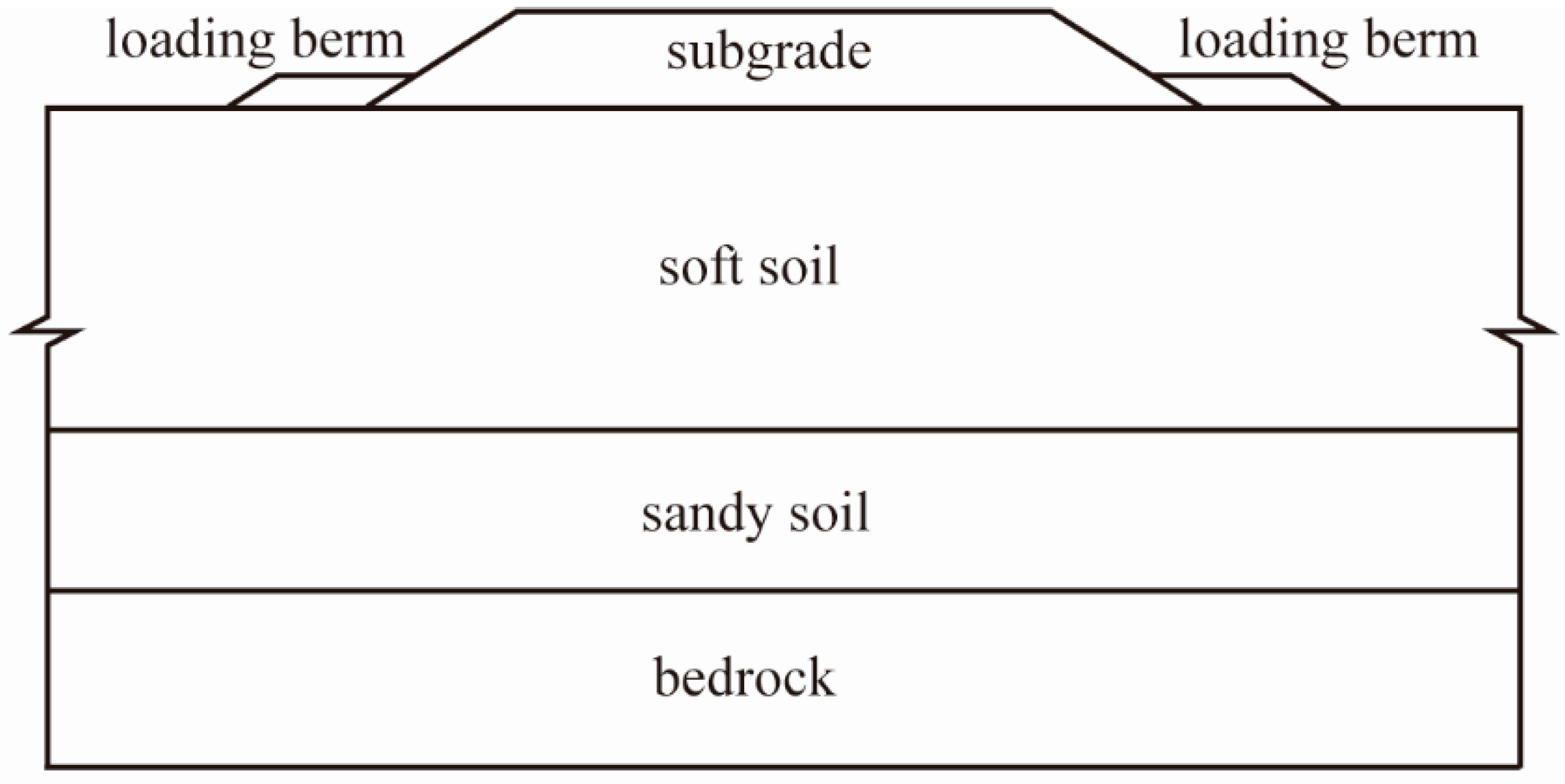
The loading berm is a treating measure of the soft soil base. The implementation method is as follows. As shown in
Figure 1, on both sides of the subgrade, the compacted soil is put on the soft soil base and then the loading berm is formed. The loading berm can inhibit the lateral uplift trend of the soft soil and improve the subgrade stability. Its effectiveness is larger than that of a cutting slope [
3]. Due to the good performance of the loading berm, it is widely used for highways in soft soil areas.
However, there are also some new cases in the loading berm application. For example, due to the large area of the loading berm, there is not enough construction space in some sections [
4]. So, the loading berm cannot be used in these sections. To address this problem, an embedded loading berm (ELB) is proposed in this paper. As shown in
Figure 2, the compacted soil is embedded into the soft soil to form the ELB. Compared to the loading berm, the ELB width is smaller. The ELB height can be increased to meet the subgrade stability requirement. The ELB can also inhibit the lateral uplift trend of the soft soil and improve the subgrade stability. Furthermore, the ELB can save construction space and reduce the disturbance effect on the surrounding environment.
To date, lots of research has been carried out on the failure modes and stability factors of subgrade in soft soil areas. These studies mainly focused on the influences of loading berm height and width on the subgrade stability factors. Zhang et al. [
4] established a stability calculation model of the highway subgrade base on the Mombasa–Nairobi Standard Gauge Railway. They concluded that the loading berm is more advantageous than the gravel pile during the construction period. Corkum et al. [
5] found that the landslide displacement can be effectively controlled by setting a small loading berm at the slope foot. Through physical modeling and field monitoring, Zaytsev et al. [
6] found that subgrade settlement can be effectively diminished by increasing the height of the loading berm. Viswanadham et al. [
7] studied the stability of the railway subgrade constructed by fly ash. The study shows that when the subgrade height is 11 m, the loading berm height should not be less than 1.5 m. Chen and Song [
8] proposed the optimization design method of a single-step loading berm and the simplified calculation method of stability factor. They also verified the applicability of the method. Zhao et al. [
9] deduced the slipping surfaces equilibrium equation considering the cohesion and internal friction angle. Based on the equilibrium equation, a method was presented for determining the reasonable width and height of the loading berm. ISAMU [
10] brought out a method to determine the dimensions of loading berm using arc law.
Recently, lots of studies were conducted on the subgrade slope stability by the numerical calculation method [
11,
12,
13,
14,
15,
16]. In 1975, Zienkiewicz et al. [
17] first applied the strength reduction method to slope stability analysis. Ma et al. [
18] researched the stability of a typical three-dimensional slope by the local strength reduction method (LSRM) and explored the feasibility of the local strength reduction method. The results show the local strength reduction method is feasible. Using the strength reduction method, Zhang et al. [
19] analyzed the stability of the subgrade with loading berm under different working conditions. The stability was compared with those calculated by the limit equilibrium method. The results show the stability calculated through the strength reduction method was closer to the actual engineering situation [
20,
21,
22].
To sum up, many scholars have carried out lots of studies on the subgrade with loading berm in soft soil areas. However, there are few studies on the stability of the highway subgrade with the ELB.
In this study, the stability of highway subgrade with the ELB was researched using analytical and numerical simulation methods. Firstly, an analytical model was proposed to describe the relationship between the ELB dimensions and the subgrade stability factors. Then, numerical simulations were carried out to reveal the stability factor of an actual subgrade with different ELB widths and heights. Lastly, the sensitivity of ELB parameters to the ELB stability factors is discussed. The research provides references for ELB design and is significant for promoting the application of ELB in soft soil areas.
3. Analytical Model for the Highway Subgrade Stability
3.1. The Relationship between the Subgrade Stability Factors and the ELB Width
The ELB and subgrade were made from compacted soil. Their strength is much greater than that of the soft soil. When the ELB strength is not enough, the subgrade is prone to shear failure as shown in
Figure 3. To quantitatively analyze the subgrade stability factor, the following assumptions are made. The position of the sliding surface does not change with the increase in subgrade width and height. That is,
h1 remains unchanged.
When the ELB cannot provide adequate resistance, subgrade shear failure will occur and the ELB breaks along the sliding surface. The ELB can be divided into two parts by the sliding surface, as shown in
Figure 4. Part I is above the sliding surface while part II is below the sliding surface. The force on part I is demonstrated in
Figure 4. The passive earth pressure on part I is
Ep. The landslide pushing force on part I from the sliding body is
Fn. The force on part I from part II is
f. When part I is in a critical state, then
The landslide body can be divided into many separate blocks. The landslide pushing force
Fn can be calculated by the limiting equilibrium theory and the transfer coefficient method. The detailed calculation process is performed using the following equation.
where
Fn,
Fn−1 are the residual sliding force of block
n and block
n − 1;
Ψn is the transfer coefficient;
Fs is the stability factor;
Gn is the weight of the block
n;
φn is the internal friction angle of the block
n along the sliding surface;
cn is the cohesion of the block
n along the sliding surface;
βn,
βn−1 are the slope angle of the block
n, block
n − 1 at the bottom, respectively;
ln is the length of the block
n along the sliding surface.
The force
f is composed of two parts. One is the cohesion on the sliding surface, and the other one is the friction on the sliding surface. Then,
In the equation, ρ is the density of the ELB body; h1 is the height of part I; c is the cohesion of the ELB body, and φ is the internal friction angle of the ELB body; B is the width of the body.
The passive earth pressure
Ep can be calculated according to the following equation.
By substituting Equations (2)–(5) into Formula (1), we obtain Equation (6).
where
For a given subgrade and the site, the physical and mechanical parameters are determined. Then, W is a constant value. In Equation (6), only Fs and B are variables. From Equation (6), it can be seen that the stability factor Fs is positively correlated with the ELB width B. With the increase in the ELB width, the subgrade stability factor Fs increases accordingly.
3.2. The Relationship between the Subgrade Stability Factors and the ELB Height
Assuming that the strength of the ELB is great enough, ELB shear failure does not occur. The overturn failure will occur as shown in
Figure 5.
Ea is the active earth pressure;
Fn is the landslide pushing force; and
E′p is the passive earth pressure.
l is the distance from the
E′p application point to the ELB bottom.
m is the distance from the
Fn application point to the ELB bottom.
When the ELB is in a critical state, the torque on the ELB equals zero. Then,
The torque equilibrium equation is established as follows.
where
,
.
The passive earth pressure
E′p can be calculated as follows.
The active earth pressure
Ea can be calculated as follows.
Substituting Equations (2), (3), (9) and (10) into Equation (8), we obtain Equation (11). Since
H is much larger than
h1,
H-
h1/2 can be replaced by
H.
where
In Equation (11), γ is soil unit weight; Ka is the active earth pressure coefficient; Kp is the passive earth pressure coefficient; Fn and Fn−1 are the residual sliding force of the block n and block n − 1, respectively; Ψn is the transfer coefficient; Fs is the stability factor; Gn is the weight of the block n; φn is the internal friction angle of block n along the sliding surface; cn is the cohesion of block n along the sliding surface; βn is the bottom slope angle of block n; ln is the length of block n along the sliding surface; h1 is the height of the ELB above the sliding surface.
Equation (11) shows that the stability factor Fs is positively correlated with the square of ELB height H. The stability factor Fs increases with the increase in the ELB height H. In a word, the stability factor Fs increases when the ELB height H and width B increase. The above analytical model can be used to design the subgrade and evaluate the subgrade stability.
There are some assumptions for the above derivation process. For example, the soil pressure on the ELB is simplified as a horizontal force. In addition, from Equations (6) and (11), it is known that there are other parameters influencing the subgrade stability, such as ELM density, cohesion, and internal friction. Therefore, it is necessary to further study the influences of these parameters on the stability factors since experimental tests have high requirements for equipment and costs [
23] and it is difficult to explore the influences of these parameters on the stability factors using Equations (6) and (11). However, numerical simulation is an efficient method to further study the influences of these parameters on the ELB stability factors.
4. Numerical Simulation for the Highway Subgrade Stability
4.1. Numerical Model
To verify the theoretical results, a numerical simulation was carried out to study the subgrade stability in this paper. The numerical model was established using Flac
3D. As shown in
Figure 6, the numerical model consists of four parts. The upper part is the subgrade; the middle part is the soft soil; the lower part is the sandy soil. There are two ELBs at the foot of the subgrade. The width of the subgrade top is 33 m; the height of the subgrade is 6 m; the subgrade slope ratio is 1:1.5; the heights of soft soil and sandy soils are 20 m and 10 m, respectively; the length of soft soil and sandy soil is 91 m. The width of the model is 1 m.
In the model, the hexahedral mesh was used for establishing all layers. Mesh sizes are 1.00 m, 1.00 m, and 1.00 m, respectively, in the X, Y, and Z directions for the soft soil and sandy soil layer. There are 91 mesh elements in the X direction, 1 mesh element in the Y direction, and 30 mesh elements in the Z direction. There are a total of 2730 mesh elements for the soft soil and sandy soil layer. At the subgrade bottom, mesh sizes are also 1 m in the X and Y directions, respectively. At the subgrade top, the total number of mesh elements is 306, which is the same as at the subgrade bottom.
As shown in
Figure 6, the X direction displacement is fixed on the left and right boundaries. The Y direction displacement is fixed on the front and back boundaries. The X, Y, and Z direction displacements are fixed on the bottom boundary. The other boundaries of the model are free. The Mohr–Coulomb constitutive model was adopted for every layer.
The physical and mechanical parameters of the model can be found with a laboratory test. The parameters of the ELB are the same as those of the subgrade. The parameters for all layers are provided in
Table 1.
4.2. Scheme of Numerical Simulation
To reveal the influences of the ELB on the subgrade stability, a study was carried out on the stability of the subgrade with different ELB widths B and heights H. The values of the ELB width are 3 m, 4 m, 5 m, and 6 m, respectively. The values of the ELB length are 5 m, 7.5 m, and 10 m, respectively. The subgrade stability factors are calculated by the strength reduction method.
The stability factor of the subgrade without the ELB was calculated first. Then, the stability factors of the subgrade with different ELB widths B and heights H were calculated. Lastly, an orthogonal test method was carried out to explore ELB parameter sensitivity to the subgrade stability.
4.3. Numerical Results and Discussion
4.3.1. The Stability of the Subgrade without and with ELB
Figure 7 shows the shear strain increment contour of the model without ELB. It can be seen that the sliding surface runs through the subgrade and the soft soil layer. That is to say, the sliding failure occurs in the model. The stability factor of the subgrade is only 1.03. It can be concluded that the subgrade is in a critical state and prone to be unstable if it is not reinforced.
Figure 8 shows the shear strain increment contour of the model with ELB. The height and width of the ELB are 6 m and 10 m, respectively.
Figure 8 demonstrates that the sliding surface does not run through the subgrade and the sliding failure does not occur in the subgrade. The stability factor of the subgrade is 1.26. This tells us that the stability of the subgrade can be improved by the ELB.
4.3.2. Influences of ELB Width on the Subgrade Stability
According to the Chinese Technical Code of Building Slope Engineering (GB50330-2013), the safety factor of the subgrade is 1.25.
Figure 9 shows the relationship between the stability factors and the ELB width. It can be seen that the stability factors of the subgrade increase with the increase in ELB width. This is agreeable with the analysis results in
Section 3.1. It is found that the stability factors of the subgrade with the ELB are greater than those of the subgrade without the ELB (
FS = 1.03). The stability factors of the subgrade with width
B = 10 m and height
H = 6 m increase by 22.33% compared with those of the subgrade without the ELB.
A linear equation was utilized to fit the relationship between the stability factors and the ELB width. The fitting formula and correlation coefficient are shown in
Table 2. When ELB height
H = 3 m, the slope of the fitting formula is 0.014. When ELB height
H = 4 m, 5 m, and 6 m, the slopes of the fitting formula are all 0.016. The correlation coefficients are higher than or equal to 0.98 for every fitting formula. The correlation coefficient is very high. It suggests that the stability factors of the subgrade increase linearly with the ELB width increase. This relationship is consistent with the analytical results in
Section 3.1.
4.3.3. Influences of ELB Height on the Subgrade Stability
Figure 10 shows the relationship between the stability factors and the ELB height (
B = 5 m,
B = 7.5 m,
B = 10 m). The stability factors increase gradually with the ELB height increase. This is also agreeable with the analytical results in
Section 3.2. The relationship between the stability factors and the ELB height was fitted using a linear equation. The fitting formula and correlation coefficients are shown in
Table 3. The correlation coefficients are equal to or more than 0.97. This implies that the linear equation is good for fitting the relationship. From
Table 3, it is seen that the slope of the fitting formula is 0.01 for the ELB width
B = 5 m and
B = 7.5 m. The slope is 0.013 for the ELB width
B = 10 m. The slopes of the fitting formula increase with the ELB width increase.
In
Table 2, the minimum slope of the fitting formula is 0.014, while the maximum slope of the fitting formula in
Table 3 is 0.013. The slope of the fitting formula in
Table 2 is greater than that in
Table 3. This means that the increased ratio of stability factors with the width increase is greater than that with the height increase. It can be concluded that the influences of ELB width on the subgrade stability factor are greater than that of ELB height. This is consistent with Chen’s research conclusion [
8].
In summary, with the ELB width and height increase, the subgrade stability factors increase. The ELB width has a greater influence on the subgrade stability factors than the ELB height. For the ELB design, the scheme with bigger ELB width is recommended to ensure subgrade stability.
5. Parameter Sensitivity Analysis
As mentioned above, there are multiple ELB parameters influencing the subgrade stability. To explore the relative influences of every parameter on the subgrade stability, the sensitivity analysis of ELB parameters is necessary to be carried out. The sensitivity analysis can be conducted by the parameter tuning method, the alternating method, the parallel line method, and the bisection method. However, these methods are not suitable for the multiple factor sensitivity analysis. So, for the ELB parameters’ sensitivity to the subgrade stability, the multiple factor methods should be used.
The orthogonal test method is a multiple-factor sensitivity analysis method. In this paper, it is used to explore the ELB parameters’ sensitivity to subgrade stability. This method combines numerical simulation with probability and statistics theory, which can reduce the test number.
5.1. Parameter Selection
The width and height are all geometric parameters. As can be seen from the above analysis in
Section 4.3, the ELB width and height have a great influence on the subgrade stability. Therefore, these geometric parameters’ sensitivity should be explored. If the ELB strength is not enough, subgrade plastic deformation and failure will occur. Therefore, the sensitivity of the physical and mechanical parameters should also be explored. In a word, the parameters selected for the sensitivity analysis are width, height, density, cohesion, and internal friction angle. The values of every parameter were determined from the value of compacted soil parameters in the literature. In this paper, the values are divided into five levels for every parameter. The parameter values for every level are shown in
Table 4.
5.2. Sensitivity Analysis
The five-factor and five-level orthogonal test was selected. There are twenty-five cases for the orthogonal test. The stability factors were calculated using the FLAC
3D software for every case. The orthogonal test scheme and stability factors are shown in
Table 5.
Kij is the sum of all test results for each factor at the same level. Rj is the range of the factor j. It can be calculated as followed
Rj = max{K1j, K2j, K3j, K4j, K5j} − min{K1j, K2j, K3j, K4j, K5j}.
The range
Rj is a variable. If the
Rj value is larger, the influences of factor
j on the subgrade stability are greater. Therefore, a larger range
Rj value indicates that the subgrade stability is more sensitive to the factor
j. The range
Rj can be used to determine the sensitivity order of every factor. The range analysis results are shown in
Table 6.
Table 6 and
Figure 11 demonstrate that
RA is the biggest,
RB,
RC, and
RD are next, and
RE is the smallest. These suggest that the ELB width is the most sensitive parameter and the internal friction is the least sensitive parameter. The ELB width’s sensitivity to the stability factors is higher than that of ELB height. This is consistent with the simulation results in
Section 4.
The RB is higher than RC. This means the sensitivity of the geometric parameters (width, height) is higher than that of the physical and mechanical parameters. The RC is higher than RD, which shows the ELB density’s sensitivity to the stability factors is higher than that of ELB cohesion. The ELB parameter sensitivity order is as follows. Width > height > density > cohesion > internal friction.
In the ELB designing process, the width and height should be focused on and the density, cohesion, and internal friction can be ignored.


