Dynamic Analysis and Structure Parameter Research on a Hydraulic Anti-Swaying System for Container Cranes

Abstract

An anti-swaying or swaying-reduction effect for a container crane is key for improving the rapidity and safety of container handling operations. By analyzing the structure of a container crane hydraulic anti-swaying system, a dynamic system model was developed in the time domain, and the changing law of the load swaying angle was studied. In order to study the attenuation effect of the load swaying angle and the different working states of the anti-swaying system, the frequency domain equation of the load swaying angle was developed in the frequency domain. A time domain study on the dynamic model shows that the structure parameter is the key parameter that affects the load anti-swaying effect, and a larger structure parameter produces a better anti-swaying effect. A study regarding the load swaying angle in the frequency domain shows that the container crane hydraulic anti-swaying system works in a critical-damping state when the structure parameter load ratio is equal to twice the system frequency, and in this case, the hydraulic anti-swaying system has good load swaying-reduction effect and a small dependence on changes in the hoisting rope length. The longitudinal and transverse installation distances of the anti-swaying fixed pulleys jointly affect the structure parameter. In engineering applications, the longitudinal and transverse distances can be selected according to size near that of a standard container. To obtain a good swaying-reduction effect, data such as the hoisting load mass, the hoisting rope length, and the hoisting load swaying speed can be obtained in real-time and used to calculate the required pressure adjustments for the relief valve of the hydraulic anti-swaying system.

1. Introduction

Container cranes comprise the primary logistics transportation equipment at railway freight yards and ports for container loading and unloading [1,2,3]. With the continuously rising global standard container transport volume and the formation of many container transport networks, the demand for container cranes would significantly increase [4,5]. Additionally, higher requirements for production efficiency and safety during container crane handling operations have been proposed [6,7]. Generally, a flexible wire rope is used to connect the trolley and the container spreader of a container crane. This kind of flexible connection can cause the load (including the container spreader and the container) and the trolley to produce up or down relative motion to meet the spatial motion requirements of the spreader or container [8,9,10]. However, due to this flexible connection and coupling relationship, when the trolley or crane starts or brakes or when there is wind resistance, the spreader (and container) swings relative to the trolley [11,12,13,14,15]. This swaying inevitably affects the rapidity and safety of the container loading and unloading operations [16,17,18].

In general, trolley-load systems are primarily considered when studying the swaying of a load [19,20]. There are two primary methods of controlling crane load swaying. The first is to take active anti-swaying measures, that is, to actively control the speed of the trolley or the crane so that the load always swings with a small swaying angle during the process of moving from a stationary position to the target position [21,22,23]. The other method is to take passive measures to reduce the swaying angle; that is, when the swaying angle is large, the trolley or the crane is passively controlled to reduce the swaying angle; thus, it is within a smaller range in the shortest possible time [24,25].

Cranes are typical representatives of symmetry-underactuated systems [26]. There is much literature about active anti-swaying measures. A finite-time regulation controller was designed for an underactuated crane system in two-dimensional (2D) space with both constant cable length and varying cable length in [27]. The finite-time technique was used to achieve simultaneous motion regulation and load swing suppression and elimination within a finite time. A dynamic differential evolutionary algorithm-based sliding-mode controller (DDE-SMC) was designed for an under-actuated crane system [28]. A model-free adaptive controller (MFAC) using feedback linearization and an adaptive fuzzy sliding mode controller (AFSMC) using fuzzy approximation were designed and employed to control an underactuated overhead crane system [29]. A time-varying gain extended state observer (ESO)-based moving sliding mode control method was proposed for anti-sway and positioning control of two-dimensional underactuated overhead cranes [30]. An accurate model-free trajectory tracking controller subject to finite time convergence for overhead crane systems was proposed based on the suitably defined non-singular terminal sliding vector [31]. A control method based on linear active disturbance rejection control (LADRC) and differential flatness theory was proposed to realize accurate trolley positioning and effective load anti-swing for the under-actuated overhead cranes in [32]. L. Ramli et al. [33] proposed an improved input shaping for minimizing the payload swing of an overhead crane with payload hoisting and payload mass variations. M. J. Maghsoudi et al. [34] proposed an optimal performance control scheme for the control of a three-dimensional (3D) crane system, including a zero-vibration shaper that considers two control objectives concurrently. The control objectives were fast and accurate positioning of a trolley and mini-mum sway of a load. An enhanced coupling PD with a sliding mode control method was proposed for the double-pendulum overhead crane systems in [35].

To summarize, more advanced control theories and methods can be adopted for active anti-swaying measures for crane loads than for passive measures. These active anti-swaying methods must design the circuit using complicated control algorithms [36,37]. In addition, it is also necessary to install corresponding sensors to measure important information, such as the trolley’s position or speed, the load swaying angle or swing angle speed, and the hoisting rope length or hoisting height [38,39]. This information is provided to the computer after digital processing, then the computer conducts operations, makes decisions, and controls the output [40,41].

The hydraulic anti-swaying system designed during this study primarily adopts passive anti-swaying measures. This hydraulic anti-swaying system has a simple structure and no complex control algorithms. Good and expected anti-swaying or swaying-reduction effects can be achieved solely with a reasonable design of the hydraulic anti-swaying system, and the hydraulic anti-swaying system frequency can avoid the frequency of natural wind [42]. Therefore, a dynamic analysis of the hydraulic anti-swaying system was conducted during this study. A dynamic model was developed within the practical engineering scope, and the main factors and key parameters affecting the anti-swaying or swaying-reduction effects were identified by simulating actual working conditions [43,44]. The purpose of this paper is to provide the theoretical basis and guidance for the specific engineering design of the hydraulic anti-swaying system.

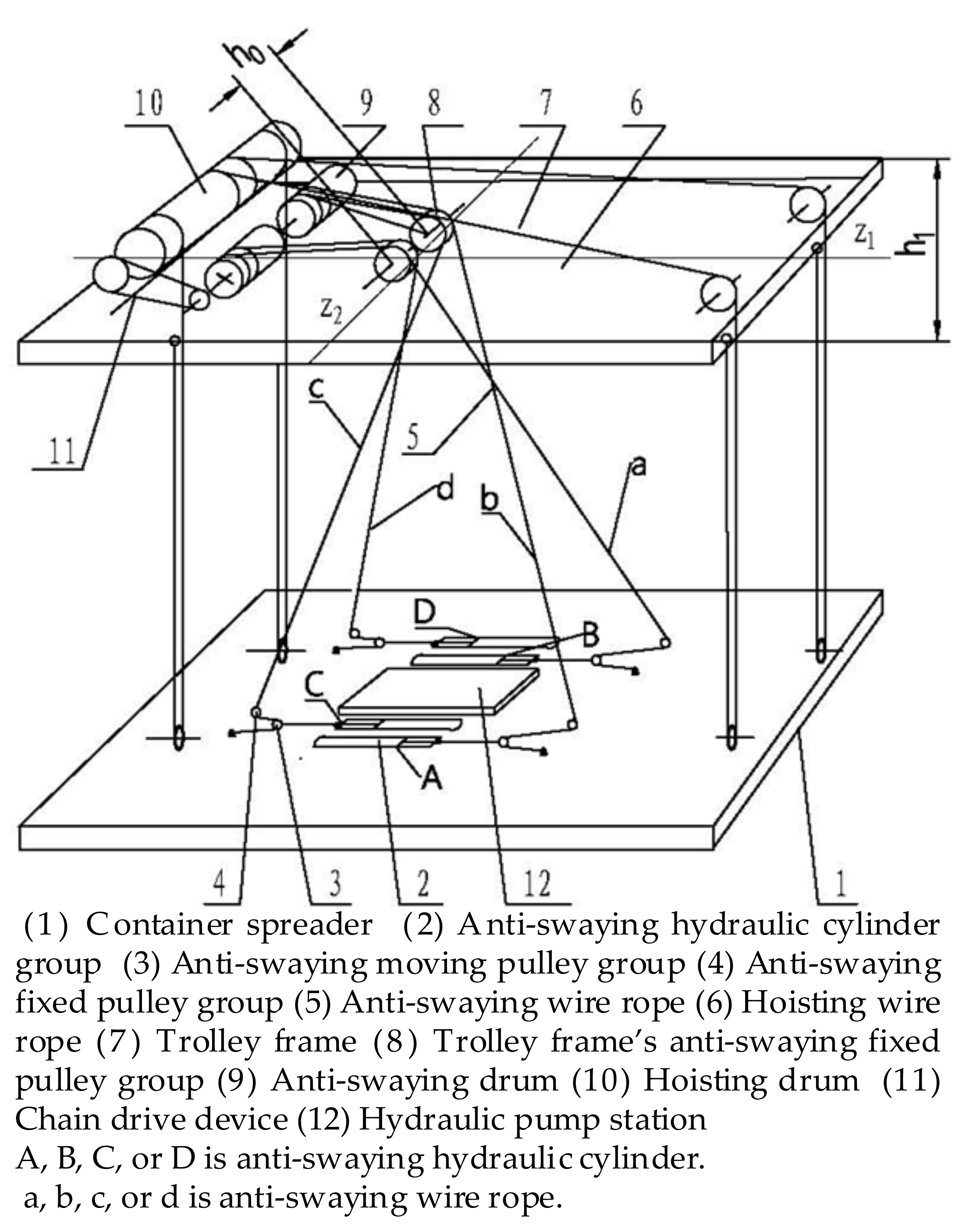
2. Mechanical Structure of the Hydraulic Anti-Swaying System

A schematic diagram of the mechanical structure of the hydraulic anti-swaying system is shown in Figure 1. Its primary components include (1) a container spreader (no container is shown below the spreader in Figure 1); (2) an anti-swaying hydraulic cylinder group (A, B, C, and D); (3) an anti-swaying moving pulley group; (4) an anti-swaying fixed pulley group mounted on the spreader; (5) an anti-swaying wire rope (a, b, c, and d); (6) a hoisting wire rope that accomplishes the hoisting function of the spreader; (7) a trolley frame rigidly connected to a running trolley (the trolley is not shown in Figure 1); (8) the trolley frame’s anti-swaying fixed pulley group installed on the trolley frame; (9) an anti-swaying drum connected to the hoisting drum by a chain drive device; (10) a hoisting drum that transfers hoisting power; (11) a chain drive device; (12) a hydraulic pump station that provides oil to the anti-swaying hydraulic cylinder group (2).

Four anti-swaying hydraulic cylinders, A, B, C, and D are symmetrically placed in the upper plane of the container spreader (1). Two of the trolley frame’s anti-swaying fixed pulleys (8) are symmetrically placed in the upper plane of the trolley frame, and their symmetry axes are z₁ and z₂ of the trolley frame (7). The installation distance, h₀, is far less than the transverse size, h₁, of the trolley frame, that is, h₀ << h₁. As shown in Figure 1, the running direction of the trolley is the longitudinal direction of the hydraulic anti-swaying system. The anti-swaying wire ropes (5) are cross-connected to the anti-swaying fixed pulley group (4) on the spreader (1) through the anti-swaying fixed pulleys (8). The anti-swaying drum (9) rotates synchronously with the hoisting drum (10) through the chain drive device (11). The rotation of the hoisting drum (10) drives the rotation of the anti-swaying drum (9) so that the hoisting rope (6) and the anti-swaying wire rope (5) extend or shorten synchronously, thereby causing the hoisting load (together with the container) to ascend or descend.

When the hoisting load does not swing, it is in a balanced position (as shown in Figure 1), the hoisting wire rope is in a vertical state, and the included angle between the hoisting wire rope and the vertical line is zero.

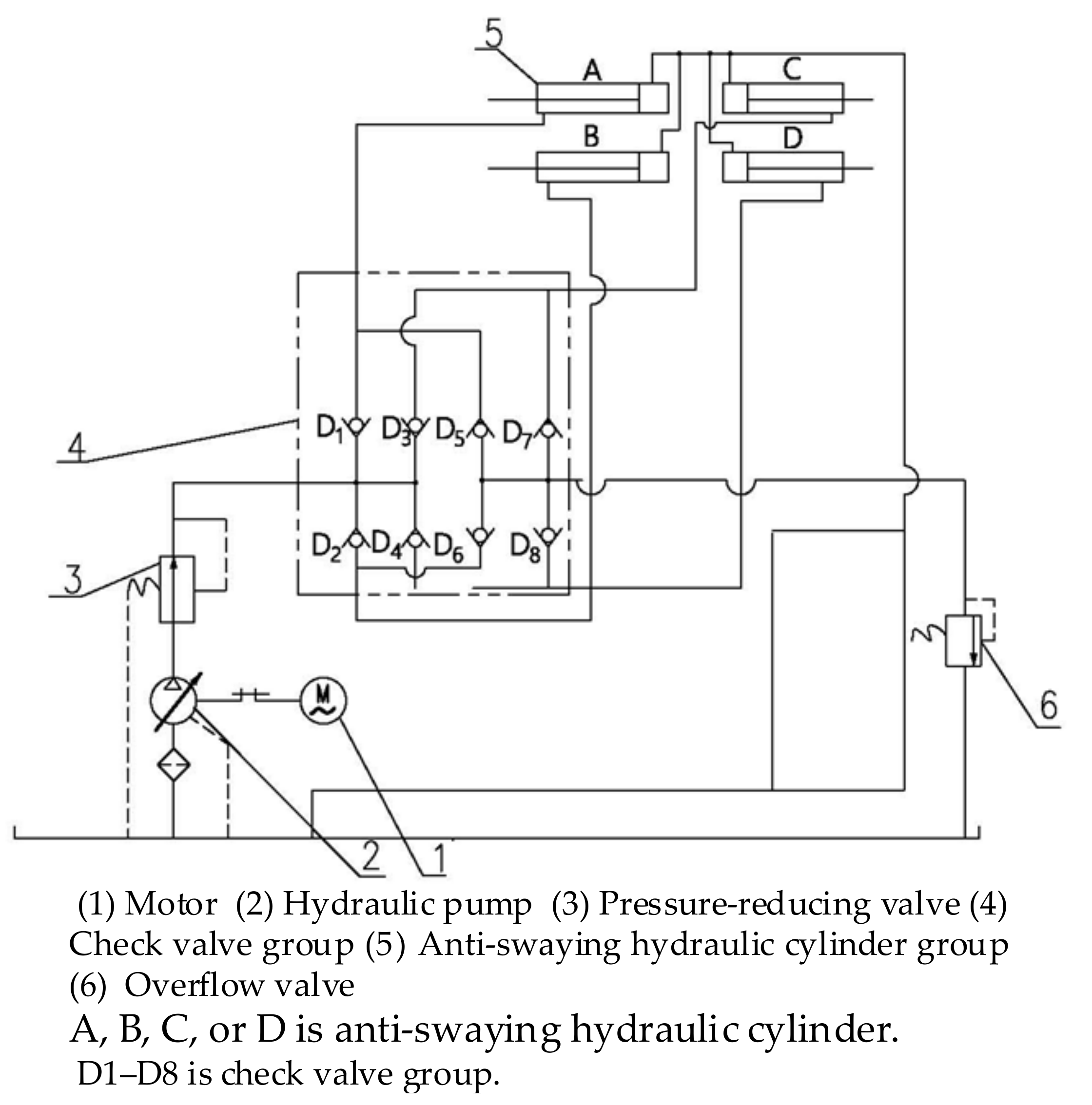
3. Principle of the Hydraulic Anti-Swaying System

A hydraulic principle diagram of the hydraulic anti-swaying system is shown in Figure 2. The hydraulic system mainly includes (1) a motor, (2) a hydraulic pump, (3) a pressure-reducing valve, (4) a check valve group (D1–D8), (5) an anti-swaying hydraulic cylinder group (A, B, C, and D), and (6) an overflow valve.

For the sake of illustration, it is assumed that the swaying of the spreader is only caused by the motion of the trolley and that the initial motion of the spreader is to the right. Once the motion begins, the tensions in the anti-swaying wire ropes a and b increase from their tensions at the initial position, so a and b are called tensioning side wire ropes. The tensions in the anti-swaying wire ropes c and d decrease from their tensions at the initial position, so c and d are called slack side wire ropes. The piston rods of cylinders A and B, which are connected to the tensioning side wire ropes a and b, extend to the side with the rod cavity under the increased tension in ropes a and b. The pressures of the rod cavity hydraulic oil in A and B increase. This pressure is greater than the outlet pressure of the pressure-reducing valve (3). Thus, check valves D1 and D2 are closed, and the oil pressures in cylinders A and B open check valves D5 and D6, respectively. When the oil pressure is greater than the set pressure of the overflow valve (6), the high-pressure oil flows back to the tank (7) through the overflow valve. At the same time, as the tensions in the slack side wire ropes c and d decrease and the oil from the pressure-reducing valve (3) opens check valves D3 and D4 and enters the rod cavities of cylinders C and D, the piston rods of cylinders C and D, which are connected to the slack side wire ropes c and d, retract toward their respective rodless cavities. Low-pressure oil flows directly back to the tank so that the slack side wire ropes c and d can remain tensioned while check valves D7 and D8 are closed. Similarly, when the hoisting load swings to the left, an analysis can be performed in accordance with the analysis method described above.

The repeated swaying of the load causes cylinders A, B, C, and D to produce the repeated motion process described above. Under the action of the check valve group (4), oil continuously spills out from the overflow valve (6), transforming the kinetic energy of the swaying load into the internal energy of the hydraulic oil buffer, thereby achieving the anti-swaying or swaying-reduction goal.

If the load swaying angle is large, the increases in the tension forces of the tensioning side wire ropes are large, and more oil would spill from the overflow valve (6). In addition, under the action of the check valve group (4), the whole hydraulic system essentially controls two hydraulic circuits with different pressures: a high-pressure circuit and a low-pressure circuit. When the load swings, as mentioned above, the high-pressure and low-pressure hydraulic circuits operate simultaneously. The oil cylinder connected to the tensioning side wire ropes causes the high-pressure circuit to be generated and the high-pressure oil to flow back to the tank through the overflow valve (6), and the oil cylinder connected to the slack side wire ropes causes the low-pressure circuit (whose pressure is determined by the pressure at the outlet of the pressure reducing valve (3) to be generated and the low-pressure oil to flow directly back to the tank. The high-pressure oil circuit in the hydraulic system is involved in the work because of the swaying of the load. If the load does not sway, when the load rises, the anti-swaying wire ropes a, b, c, and d are all in a tensioned state. When the load descends, the anti-swaying wire ropes a, b, c, and d are all in a relaxed state, the outlet oil of the pressure-reducing valve (3) simultaneously opens check valves D1, D2, D3, and D4, and then flows into the rod cavity of cylinders A, B, C, and D. At this time, since the oil pressure cannot reach the set pressure of the overflow valve (6), it cannot open the overflow valve (6), and the oil in the four cylinders’ rodless cavities can only flow directly into the tank. The oil rapidly pushes the pistons toward the rodless cavities of the respective cylinders so that the low-pressure circuit ensures that the anti-swaying wire ropes ascend and descend synchronously with the hoisting rope, with little resistance and rapid tensioning of the four anti-swaying wire ropes.

When the load sways to its highest position, the swaying angle is the largest, and the swaying angle velocity and swaying speed of the load are zero. At this time, the resistance in the high-pressure circuit of the hydraulic system must be as small as possible so that the load can quickly return to its balanced position, namely its lowest point. Furthermore, when the load sways to its lowest position, the swaying angle is zero, and the swaying angle velocity and swaying speed of the load may both be at a maximum. At this time, the high-pressure circuit of the hydraulic system must provide maximum pressure so that the kinetic energy of the swaying of the load can be converted into internal energy of the hydraulic oil buffer. Therefore, the basic requirement for the hydraulic system is that the oil pressure in the high-pressure circuit must change with changes in the swaying angle velocity or the swaying speed of the load.

4. Time Domain Dynamic Equations for the Anti-Swaying System

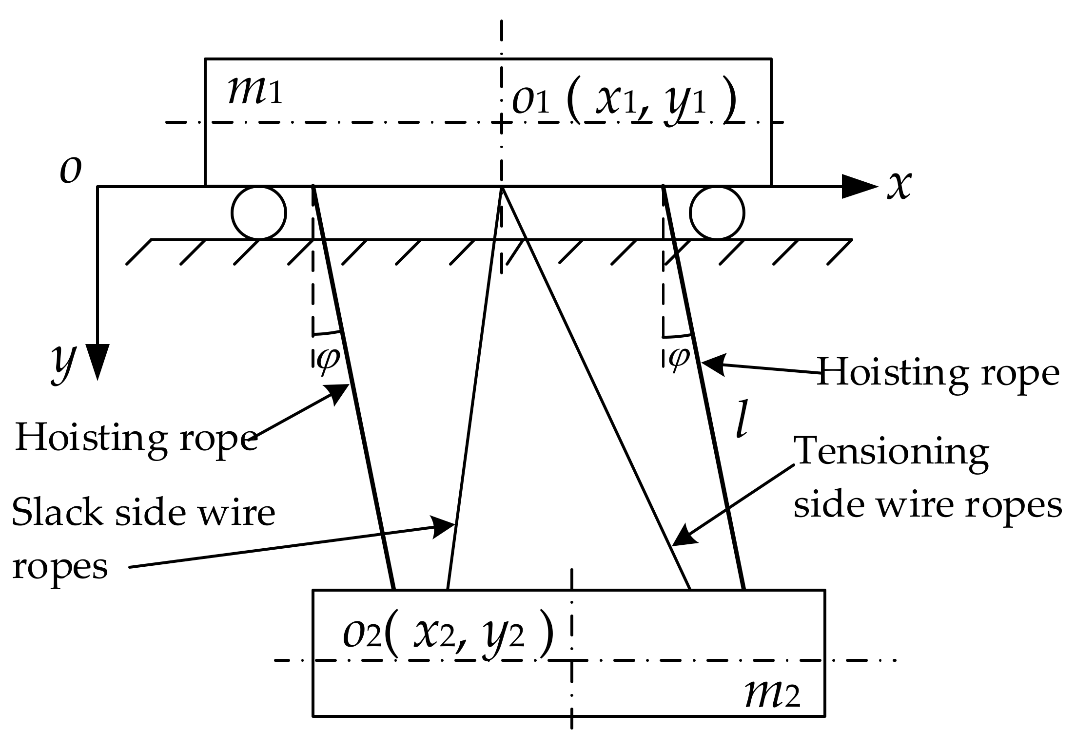
4.1. Dynamic Analysis of the Anti-Swaying System

In general, when there is no wind load, the influences of the trolley and the crane on the load swaying are the same. Therefore, for the sake of convenience, only the trolley–crane coupling structure was considered in this study. As mentioned previously, the installation distance, h₀, of the two-trolley frame anti-swaying fixed pulleys (8) is much smaller than the transverse size, h₁, of the trolley frame, that is, h₀ << h₁. Therefore, it can be assumed that the four anti-swaying ropes, a, b, c, and d, are suspended at a point P through the trolley frame fixed pulleys; the projection of the suspension point P on the spreader is the intersection point Q, and point Q is the intersection of the rectangular diagonals determined by the spreader fixed pulley group (4). Suppose the load sways to the right with an angle of φ (rad). A schematic diagram of the simplified structure of the crane and trolley–load system is shown in Figure 3. When the load does not swing, that is, when φ = 0, the spatial layout of the anti-swaying wire ropes a, b, c, and d is shown in Figure 4, where θ₁ represents the angle between the anti-swaying wire ropes and the mounting plane angle of the anti-swaying fixed pulleys. It is clear that θ₁ depends on the height of the load, that is, the length of the hoisting rope when the load does not swing but is in its equilibrium position. θ₂ is determined by the installation positions of the anti-swaying fixed pulleys on the spreader. e and f are determined by the installation positions of the anti-swaying fixed pulleys. e represents the installation distance of the anti-swaying fixed pulleys in the running direction of the trolley, referred to as the longitudinal distance of the anti-swaying fixed pulleys. f is the installation distance of the anti-swaying fixed pulleys in the direction perpendicular to the running direction of the trolley, referred to as the transverse distance of the anti-swaying fixed pulleys. The units of e and f are both m. G(t) represents the sum of the tensions in the two tensioning side wire ropes. F_x is the sum of the horizontal components of the forces the two tensioning side wire ropes exert on the load. The units of G(t) and F_x are both N. It is clear that G(t) = F_x, and F_x is also the force exerted by the cylinder connected to the tensioning side anti-swaying wire ropes.

In addition, for the convenience of the study, the following simplifications and approximate hypotheses were made:

(1)

The load swaying is similar to the swinging of a single pendulum and is longitudinal swinging when the influences of starting and braking are considered. The load swaying angle is φ and does not exceed 5°, namely, φ ≤ 5°;

(2)

According to the basic requirement of the hydraulic system, the oil pressure in the high-pressure circuit of the hydraulic system changes with changes in the load-swaying speed. The horizontal component, F_x, of the force that the anti-swaying wire ropes exert on the load is approximately proportional to the load-swaying speed. During swaying, the anti-swaying wire ropes on the tensioning side are affected by F_x. Considering the structural characteristics of the hydraulic anti-swaying system and the lag factor caused by hydraulic damping, the force that the slack side wire ropes exert on the load is not considered. Considering that the load swaying angle, φ, is smaller than both θ₁ and θ₂, it can be assumed that the force that the anti-swaying wire ropes exert on the load is constant;

(3)

The weights of the anti-swaying wire ropes, the friction between the wheel and the rail, wind resistance, and air damping are ignored. The cross-sectional areas of the piston rods of the anti-swaying hydraulic cylinders are also not considered.

The trolley and the load (including the spreader and the container) can be represented by m₁ and m₂, respectively, in units of kg. Since the mass of the spreader is less than that of the container, m₂ is determined only by the mass of the container, and m₂ is also referred to as the load. The coordinates of the centroids of m₁ and m₂ in the Oxy coordinate system in Figure 3 are O₁(x₁, y₁) and O₂(x₂, y₂), respectively. The hoisting rope length is represented by l, which has units of m. The location of zero potential energy was selected as the horizontal plane where the O_x axis lies. The system’s potential energy is expressed by $-m_{2}gl\cos \phi$. If the trolley position, x₁, the load swaying angle, φ, and the hoisting rope length, l, are selected as generalized coordinates, then Equation (1) can be written as:

$$\left\{\begin{array}{c}{y}_1=0\hfill \\ y_2=x_1-l\sin \phi \hfill \\ y_2=l\cos \phi \hfill \end{array}\right..$$

(1)

The load swaying speed is expressed by Equation (2):

$$v_2=\sqrt{{\dot{x}}_1^2+2{\dot{x}}_1\dot{l}\sin \phi +2l{\dot{x}}_1\dot{\phi }\cos \phi +{\dot{l}}^2+l^2{\dot{\phi }}^2}.$$

(2)

According to Equations (1) and (2), the system Lagrange function and the Lagrange equations are given by Equations (3) and (4), respectively.

$$\begin{array}{c}L=\frac{1}{2}\left(m_1+m_2\right){\dot{x}}_1^2+m_2{\dot{x}}_1\dot{l}\sin \phi +m_{2}l{\dot{x}}_1\dot{\phi }\cos \phi +\frac{1}{2}{m}_2{\dot{l}}^2\\ +\frac{1}{2}{m}_2{l}^2{\dot{\phi }}^2+m_{2}gl\cos \phi \end{array}$$

(3)

In Equation (3), g represents the acceleration of gravity, equal to 9.81 m/s².

$$\frac{\mathrm{d}}{\mathrm{d}t}\frac{\partial L}{\partial {\dot{q}}_i}-\frac{\partial L}{\partial q_i}=F_{q_i}\begin{array}{cc}& \end{array}\left(i=1,2,3\right)$$

(4)

In Equation (4), q_i represents the generalized coordinate (q₁ = x₁, q₂ = φ, q₃ = l); $F_{q_i}$ is the generalized force, $F_{q_1}=F\left(t\right)$ is the driving force of the trolley, and $F_{q_2}=-G\left(t\right)l\cos {\theta }_1\cos {\theta }_2\cos \phi$ and $F_{q_3}=F_l\left(t\right)$ is the hoisting force of the load.

According to hypothesis (2), Equation (5) can be obtained:

$$F_x=\lambda v_2$$

(5)

where λ is a proportional constant, with units of N • s • m⁻¹, that depends on the high-pressure loop pressure of the hydraulic system, and λ > 0. It is clear that λ depends on the pressure of the overflow valve (6) when the structure and size of the anti-swaying hydraulic cylinders A, B, C, and D are determined.

After substituting Equations (2), (3), and (5) into Equation (4), the system dynamics equation could be obtained:

$$\mathit{A}\left(\mathit{q}\right)\ddot{\mathit{q}}+\mathit{B}\left(\mathit{q},\dot{\mathit{q}}\right)\dot{\mathit{q}}+\mathit{C}\left(\mathit{q}\right)=\mathit{u}$$

(6)

where, $\mathit{q}={[\begin{array}{ccc}{x}_1& \phi & l\end{array}]}^T$, $\mathit{C}\left(\mathit{q}\right)={[\begin{array}{ccc}0& 2m_{2}gl\sin \phi & m_{2}g\cos \phi \end{array}]}^T$, $\mathit{u}={[\begin{array}{ccc}F\left(t\right)& -kl{v}_2\cos \phi & F_l\left(t\right)\end{array}]}^T$, $\mathit{A}\left(\mathit{q}\right)=\left[\begin{array}{ccc}{m}_1+m_2& m_{2}l\cos \phi & m_2\sin \phi \\ m_{2}l\cos \phi & m_2{l}^2& 0\\ m_2\sin \phi & 0& m_2\end{array}\right]$,$\mathit{B}\left(\mathit{q},\dot{\mathit{q}}\right)=\left[\begin{array}{ccc}0& m_2\left(\dot{l}\cos \phi -l\dot{\phi }\sin \phi \right)& m_2\dot{\phi }\cos \phi \\ 0& m_2\dot{l}& m_2\dot{\phi }\\ 0& -m_{2}l\dot{\phi }& 0\end{array}\right]$, and

$$k=\lambda \cos {\theta }_1\cos {\theta }_2$$

(7)

In Equation (7), k represents the structure parameter of the hydraulic anti-swaying system, termed the structure parameter for conciseness, and $k>0$. It is clear that k primarily depends on the installation positions of the hydraulic system and the anti-swaying fixed pulley group (4) on the spreader (1).

4.2. Equation for the Load Swaying Angle

For the convenience of analysis, it is assumed that the hoisting rope length, l, is constant, leading to $\dot{l}=\ddot{l}=0$. When the trolley brakes, the following expression can be obtained from Equation (6):

$$\begin{array}{c}{m}_{2}l\left(m_2{\sin }^2\phi \left(t\right)+m_1\right)\ddot{\phi }\left(t\right)+\frac{1}{2}{m}_2^{2}l\sin (2\phi \left(t\right)){\dot{\phi }}^2\left(t\right)+\\ k\left(m_1+m_2\right)v_2\cos \phi \left(t\right)+2m_{2}g\left(m_1+m_2\right)\sin \phi \left(t\right)=0\end{array}$$

(8)

If φ ≤ 5°, then $\sin \phi =\phi$, $\cos \phi =1$, and the higher-order trace containing ${\dot{\phi }}^2$ can be ignored. At the same time, when the trolley is stationary after braking, ${\ddot{x}}_1={\dot{x}}_1=0$ applies. According to Equation (2), $v_2=l\dot{\phi }$ holds. Thus, Equation (9) can be obtained from Equation (8):

$$\ddot{\phi }\left(t\right)+Mk\dot{\phi }\left(t\right)+2M{m}_2\frac{g}{l}\phi \left(t\right)=0,$$

(9)

where $M=\frac{1}{m_1}+\frac{1}{m_2}$ M, m₁, m₂, and l are dynamic parameters of the trolley–load system.

To study the change trend for the load swaying angle when the trolley brakes (t = 0), the load swaying angle and its derivative were set to $\phi \left(0\right)={\phi }_0$ (${\phi }_0$ is the initial swaying angle during braking) and $\dot{\phi }\left(0\right)=0$. When $M{k}^{2}l-4m_2^{2}g>0$, based on Equation (9), it was concluded that the change trend for the swaying angle of the load could be expressed by Equation (10):

$$\phi \left(t\right)={\xi }_1{e}^{-\alpha t}-{\xi }_2{e}^{-\beta t},$$

(10)

where ${\xi }_1=\frac{{\phi }_0\left(M{k}^{2}l+\gamma -8m_{2}g\right)}{2\omega }$, ${\xi }_2=\frac{{\phi }_0\left(M{k}^{2}l-\gamma -8m_{2}g\right)}{2\omega }$, $\alpha =\frac{Mkl-\frac{\gamma }{k}}{2l}$, $\beta =\frac{Mkl+\frac{\gamma }{k}}{2l}$, $\gamma =k\sqrt{{(Mkl)}^2-8M{m}_{2}gl}$, and $\omega =\sqrt{M{k}^{2}l-8m_{2}g}$.

Equation (10) is the expression for the load swaying angle after the trolley brakes. It is clear that the load swaying angle is attenuated in the form of an exponential function. Equations (9) and (10) indicate that the structure parameter, k, the hoisting load, m₂, and the hoisting rope length, l, jointly affect the attenuation process of the initial swaying angle, ${\phi }_0$.

5. Dynamic Equation for the Anti-Swaying System in the Frequency Domain

Based on Equation (10), the structure parameter k significantly influences the swaying-reduction effect of the hydraulic anti-swaying system. Then, the k value must be determined in such a way that the swaying-reduction effect of the hydraulic anti-swaying system can reach an ideal state.

In Equation (9), let $Mk=\epsilon$. $\epsilon$ is called the structure parameter load ratio and has units of Hz. By performing a Laplace transform on Equation (9), a complex domain function for the load swaying angle can be obtained:

$$\Phi \left(s\right)=\frac{\left(s+2\xi {\omega }_n\right){\phi }_0}{s^2+2\xi {\omega }_{n}s+{\omega }_n^2}.$$

(11)

In Equation (11), s is a complex variable and $s=\sigma +j\tau$. $\sigma$ and $\tau$ are real variables, and j is an imaginary unit. ${\omega }_n=\sqrt{\frac{2M{m}_{2}g}{l}}$ is the system frequency in units of Hz, m₁, m₂, and l together affect the system frequency. $\xi =\frac{\epsilon }{2{\omega }_n}$ is called the dimensionless damping coefficient, or the damping coefficient for conciseness, and $\xi >0$. Equation (12) is an obvious result of these definitions:

$$\xi =\frac{k}{2}\sqrt{\frac{Ml}{2m_{2}g}}$$

(12)

The denominator in Equation (11) can be set equal to zero, as in Equation (13):

$$s^2+2\xi {\omega }_{n}s+{\omega }_n^2=0$$

(13)

Equation (13) is called the characteristic equation of the hydraulic anti-swaying system, and the corresponding root of Equation (13) is called the characteristic root of the hydraulic anti-swaying system.

The following list discusses the system operation for different value ranges of the damping coefficient, $\xi$.

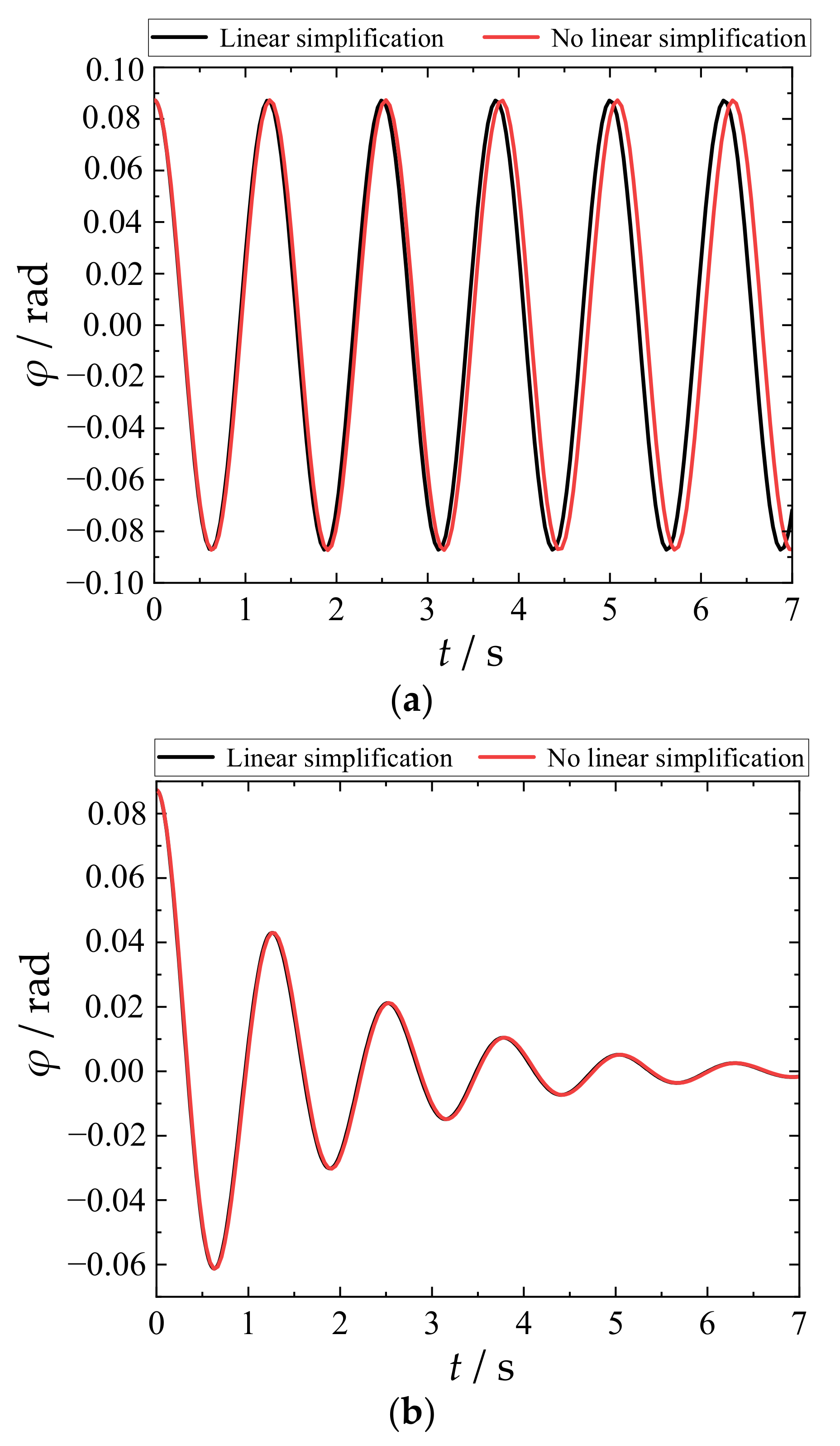
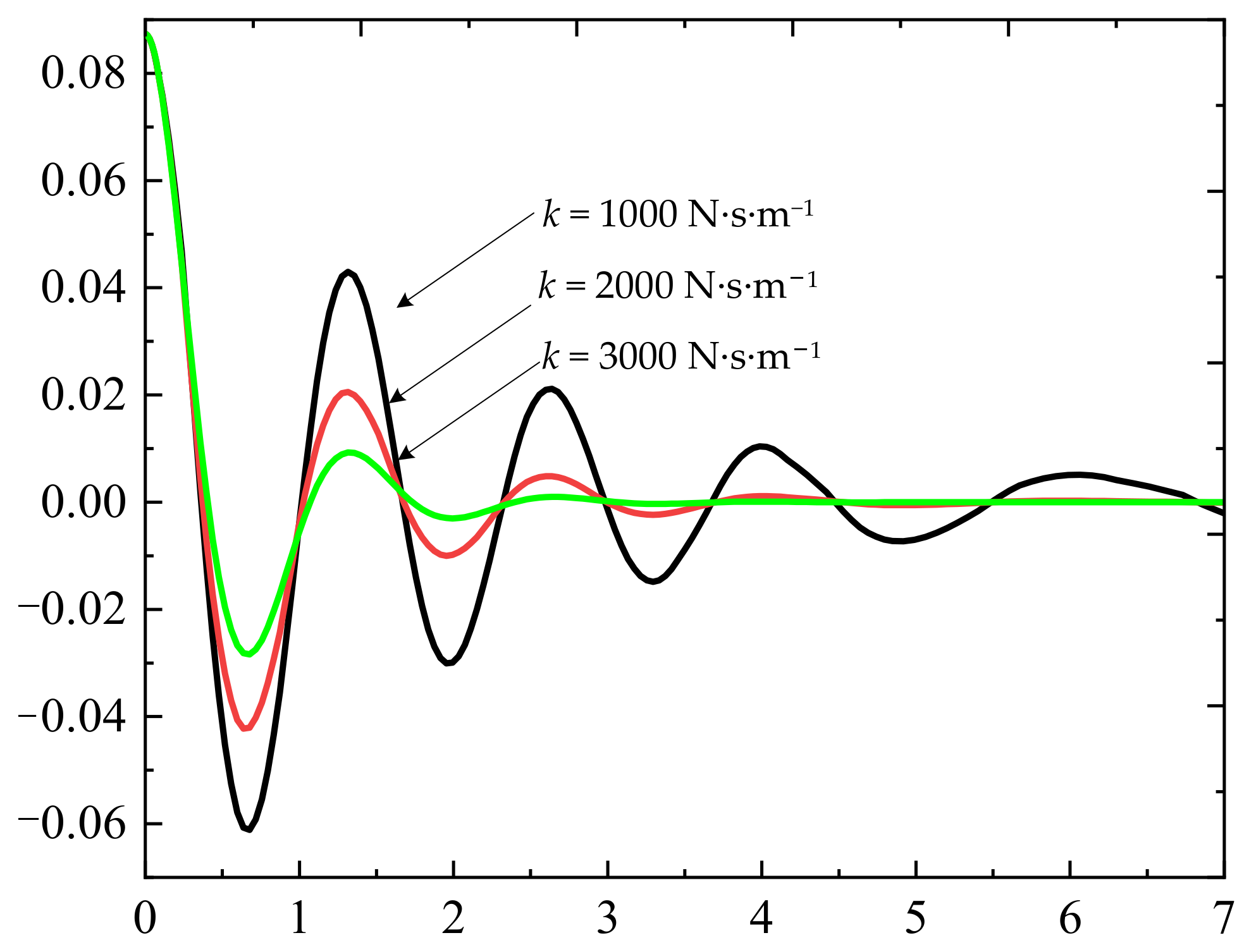
5.1. Under-Damping Hydraulic Anti-Swaying System

When $0<\xi <1$, that is, when $0<\epsilon <2{\omega }_n$, the anti-swaying system is called an under-damping hydraulic anti-swaying system. In this situation, Equation (13) has two conjugate complex characteristic roots:

$$s_{1,2}=-\xi {\omega }_n\pm j{\omega }_n\sqrt{1-{\xi }^2}.$$

(14)

Then, the time domain function of the load swaying angle can be expressed by Equation (15):

$$\phi \left(t\right)=\frac{{\phi }_0}{\sqrt{1-{\xi }^2}}{e}^{-\xi {\omega }_n^t}\sin ({\omega }_n\sqrt{1-{\xi }^2}t+{\mathit{cos}}^{-1}\xi ).$$

(15)

It is clear that Equations (10) and (15) are equivalent when the hydraulic anti-swaying system is an under-damping hydraulic anti-swaying system. When ${\phi }_0$ and ${\omega }_n$ are known, Equation (15) shows that the change in the swaying angle with time is only affected by the damping coefficient, $\xi$. Based on Equation (10), the entire oscillatory attenuation process experienced by the swaying angle is always contained between a pair of envelope surfaces, $\pm \frac{{\phi }_0}{\sqrt{1-{\xi }^2}}{e}^{-\xi {\omega }_{n}t}$.

The attenuation time of the swaying angle is an important index for measuring the effect of the anti-swaying system. If the load swaying angle is required to attenuate to $\Delta$ (rad) at $t_s$ (i.e., the distance between the envelope surfaces is $\Delta$), then Equation (16) applies:

$$\frac{2{\phi }_0}{\sqrt{1-{\xi }^2}}{e}^{-\xi {\omega }_n^t}=\Delta .$$

(16)

According to Equation (16), the attenuation time of the load swaying angle can be expressed by Equation (17):

$$t_s=\frac{\ln \frac{{\Delta }^2\left(1-{\xi }^2\right)}{4{\phi }_0^2}}{2\xi {\omega }_n}.$$

(17)

5.2. Critical-Damping Hydraulic Anti-Swaying System

When $\xi =1$, that is, when $\epsilon =2{\omega }_n$, the anti-swaying system is called a critical-damping hydraulic anti-swaying system, and Equation (13) has characteristic roots of double real numbers equal to $-{\omega }_n$. In this situation, the time domain function of the load swaying angle can be expressed by Equation (18):

$$\phi \left(t\right)=\left(1+{\omega }_{n}t\right){\phi }_0{e}^{-{\omega }_{n}t}.$$

(18)

Equation (18) shows that the swaying angle attenuates exponentially. When M is known, the anti-swaying effect of the system is only affected by the length, l, of the hoisting rope.

5.3. Over-Damping Hydraulic Anti-Swaying System

When $\xi >1$, that is, when $\epsilon >2{\omega }_n$, the anti-swaying system is called an over-damping hydraulic anti-swaying system, and Equation (13) has two real characteristic roots:

$$s_{1,2}=-\xi {\omega }_n\pm j{\omega }_n\sqrt{{\xi }^2-1}.$$

(19)

Then, the time domain function for the load swaying angle can be expressed by Equation (20):

$$\phi \left(t\right)={\phi }_0{e}^{-\xi {\omega }_{n}t}\{\mathit{cos}\mathrm{h}[{\omega }_n\sqrt{{\xi }^2-1}t]-\frac{\mathit{sin}\mathrm{h}[{\omega }_n\sqrt{{\xi }^2-1}t]\left(\xi -2\right)}{\sqrt{{\xi }^2-1}}\}.$$

(20)

To make the hydraulic anti-swaying system have a good anti-swaying effect and a low dependence on the length of the hoisting rope, the structure parameter load ratio must generally be equal to twice the system frequency, ${\omega }_n$, in engineering applications, that is, the system must work in the critical-damping state. According to the definition of the structure parameter load ratio, $Mk=\epsilon$, at this point, the relationship between the structure parameter, k, and the dynamic parameters of the trolley–load system should be expressed by Equation (21):

$$k=2\sqrt{\frac{2m_{2}g}{Ml}}.$$

(21)

6. Determination of the Structure Parameter and the Hydraulic System Pressure

When the hydraulic anti-swaying system works in the critical-damping state, the hoisting rope length, l, can be considered a constant due to the independence of the anti-swaying effect of the system from changes in the hoisting rope length. Equation (22) can then be obtained from Figure 4:

$$\left\{\begin{array}{c}\cos {\theta }_1=\frac{\sqrt{e^2+f^2}}{\sqrt{4l^2+e^2+f^2}}\hfill \\ \cos {\theta }_2=\frac{e}{\sqrt{e^2+f^2}}\hfill \end{array}\right..$$

(22)

Then, Equations (7) and (22) could be used to obtain Equation (23):

$$k=\frac{\lambda }{\sqrt{4{(\frac{l}{f})}^2+{(\frac{e}{f})}^2+1}}.$$

(23)

The proportional constant can be obtained from Equations (21) and (23):

$$\lambda =2\sqrt{\frac{2m_{2}g}{Ml}}\cdot \sqrt{4{(\frac{l}{f})}^2+{(\frac{e}{f})}^2+1}.$$

(24)

The expression in Equation (25) is then briefly considered:

$$F_x=p_{x}S,$$

(25)

where $p_x$ represents the set pressure of the overflow valve (6) in units of MPa, and S is the cross-sectional area of the anti-swaying hydraulic cylinder with units of m².

Finally, Equation (26) can be obtained from Equations (5) and (25):

$$p_x=\frac{2\sqrt{\frac{2m_{2}g}{Ml}}\cdot \sqrt{4{(\frac{l}{f})}^2+{(\frac{e}{f})}^2+1}}{S}{v}_2$$

(26)

According to Equation (26), the setting pressure, $p_x$, of the overflow valve (6) can be calculated in real-time through field measurements of m₂, l, and v₂, so that the hydraulic anti-swaying system can achieve a good anti-swaying effect.

7. Calculation Example

Based on the actual crane operating conditions, the simulation experiment parameters are given: $m_1=1000 \mathrm{kg}$, $m_2=1000-\mathrm{10,000} \mathrm{kg}$ (including the spreader), $l=1-8 m$, and ${\phi }_0=5^{\circ }$. By calculation, the system frequency is ${\omega }_n=4.6-14.7 \mathrm{Hz}$. Based on Equation (11), as the length l of the rope decreases, the system frequency will increase when the weight is lifted. So, the system frequency can avoid the frequency of natural wind.

To illustrate the effectiveness of the linear simplification involved in moving from Equation (8) to Equation (9), simulation verification results are presented in Figure 5. Figure 5a shows the dynamic response process for the load swaying angle when there is no hydraulic anti-swaying system (k = 0), and Figure 5b shows the dynamic response process for the load swaying angle when the hydraulic anti-swaying system is implemented (k ≠ 0). Figure 5 indicates that the linear simplification is reasonable and effective.

Based on Equations (9) and (10), when M and l are known, k significantly influences the attenuation of the swaying angle, as shown in Figure 6. Figure 6 shows that a larger k value is conducive to the attenuation of the swaying angle. However, according to Equation (7), a larger k value means that the hydraulic system would provide a larger oil pressure.

Figure 7 shows the influence of the damping coefficient of the under-damping hydraulic anti-swaying system on the attenuation of the swaying angle. Equation (15) and Figure 7 indicate that the swaying angle of the under-damping hydraulic anti-swaying system experiences an oscillatory attenuation process during which the amplitude changes with time. When the damping coefficient, $\xi$, is smaller, the oscillation is more obvious, indicating that the container oscillates more significantly, which is not allowed in engineering practice. Meanwhile, the entire oscillatory attenuation process experienced by the swaying angle is always contained between a pair of envelope surfaces, $\pm \frac{0.085}{\sqrt{1-{\xi }^2}}{e}^{-12.8\xi t}$, as shown in Figure 8. Figure 8 shows that a larger damping coefficient, $\xi$, leads to a more rapid convergence of the envelope surfaces to zero, indicating that the oscillation in Figure 7 is weaker and that the swaying angle attenuation is faster, so the anti-swaying effect of the anti-swaying system is better.

According to Equation (17), when $\Delta$ and ${\phi }_0$ are known, the attenuation time, $t_s$, of the swaying angle is determined by the damping coefficient, $\xi$, and the length of the hoisting rope. Figure 9 illustrates this conclusion. Figure 9 also shows that when $\xi$ increases, $t_s$ decreases from fast to slow. If $\xi$ is small, then $t_s$ increases as l increases; if $\xi$ is large, then $t_s$ remains nearly constant as l changes, indicating that when $\xi$ is large, the anti-swaying effect of the system has a certain robustness to the changes in l.

Figure 10 shows the influence of the hoisting rope length, l, of the critical-damping hydraulic anti-swaying system on the anti-swaying effect. Figure 10 indicates that the critical-damping system has a good anti-swaying effect, and its anti-swaying effect is less dependent on the changes in the hoisting rope length, l.

Figure 11 shows the changes in the swaying angle with time for the over-damping hydraulic anti-swaying system as the damping coefficient, $\xi$, changes. Figure 10 also shows that the damping effect, $\xi$, is visibly worse than that of the critical-damping anti-swaying system.

A comparison of Figure 7, Figure 10 and Figure 11 shows that, at the same system frequency of the anti-swaying system, with increases in the damping coefficient, $\xi$, the attenuation of the load swaying angle changes from oscillation attenuation to exponential attenuation to hyperbolic sinusoidal (or hyperbolic cosine) attenuation successively.

According to Equation (23), when the pressure and size of the anti-swaying hydraulic cylinders A, B, C, and D in the hydraulic system are determined, the longitudinal distance, e, and the transverse distance, f, of the anti-swaying fixed pulleys jointly affect the structure parameter, k. As shown in Figure 12, when f decreases or e increases, k is likely to increase, which is favorable for the load anti-swaying effect. In engineering applications, if common standard containers and anti-swaying cylinders that are convenient to install are considered, $e=6m$ and $f=2.5m$ can be selected.

8. Conclusions

In this study, it was found that a reasonable design and proper selection of the structure parameter for a container crane hydraulic anti-swaying system were the keys to obtaining a good anti-swaying effect for the load. By developing a dynamic model for the hydraulic anti-swaying system and conducting dynamic research in the time and frequency domains, the following important conclusions were obtained:

(1)

The action of the high-pressure circuit of the hydraulic system, combined with the anti-swaying rope, could attenuate the swaying angle of the load, thereby achieving the anti-swaying purpose for the load. The structure parameter primarily affected the load anti-swaying effect, and a larger structure parameter produced a better anti-swaying effect. The structure parameter depended on the hydraulic system itself and the installation position of the anti-swaying fixed pulley group;

(2)

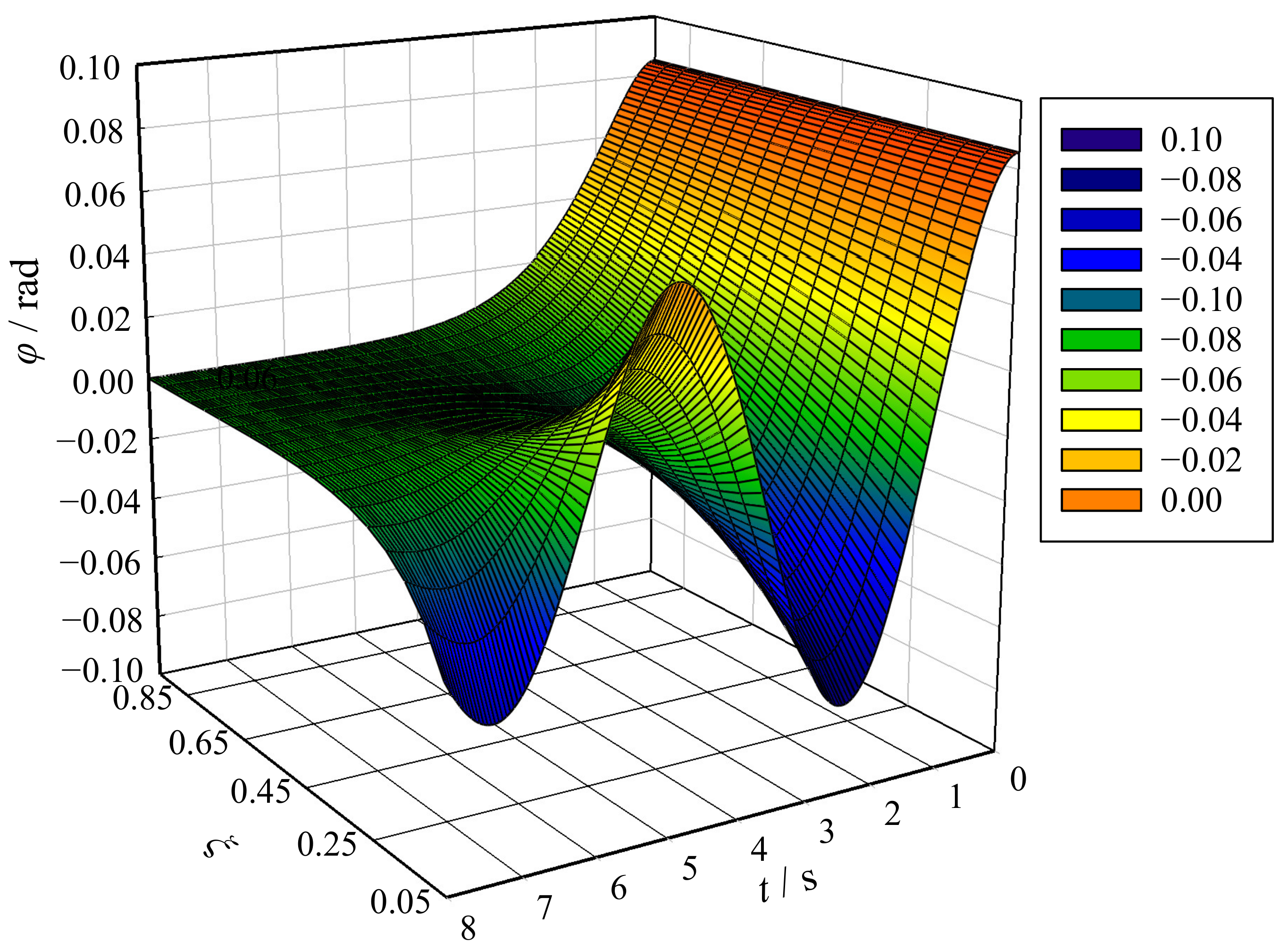
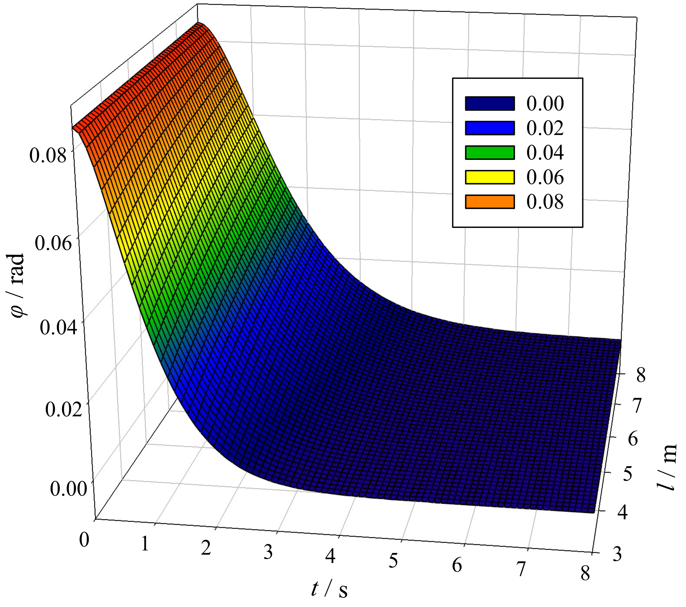
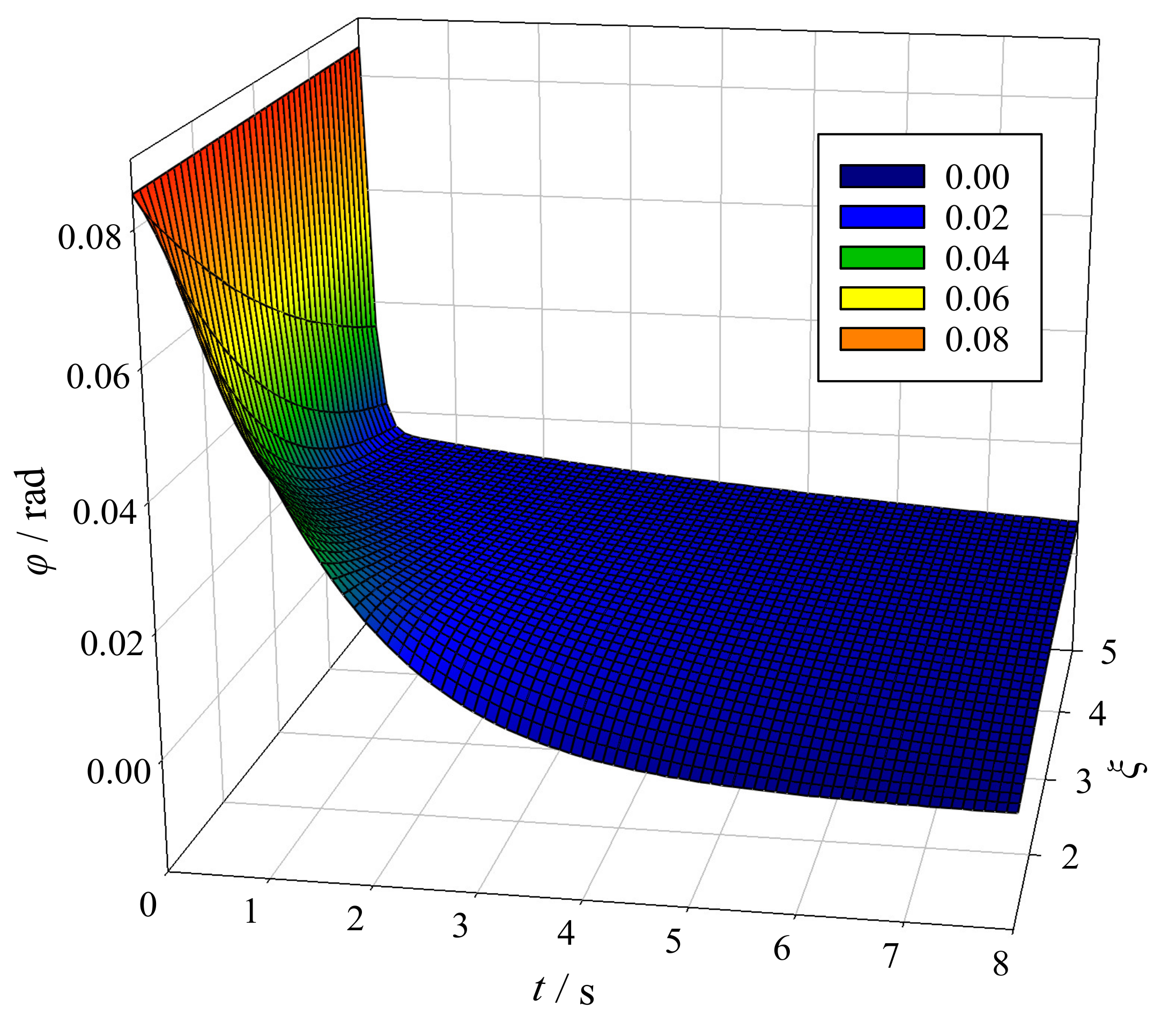
Different structure parameter load ratios could cause the hydraulic anti-swaying system to work in under-damping, critical-damping, or over-damping states. For engineering applications, the hydraulic anti-swaying system could be made to work in the critical-damping state because the critical-damping anti-swaying system produced a good anti-swaying effect with less dependence on changes in the hoisting rope length. The structure parameter load ratio for the critical-damping system was twice the system frequency;

(3)

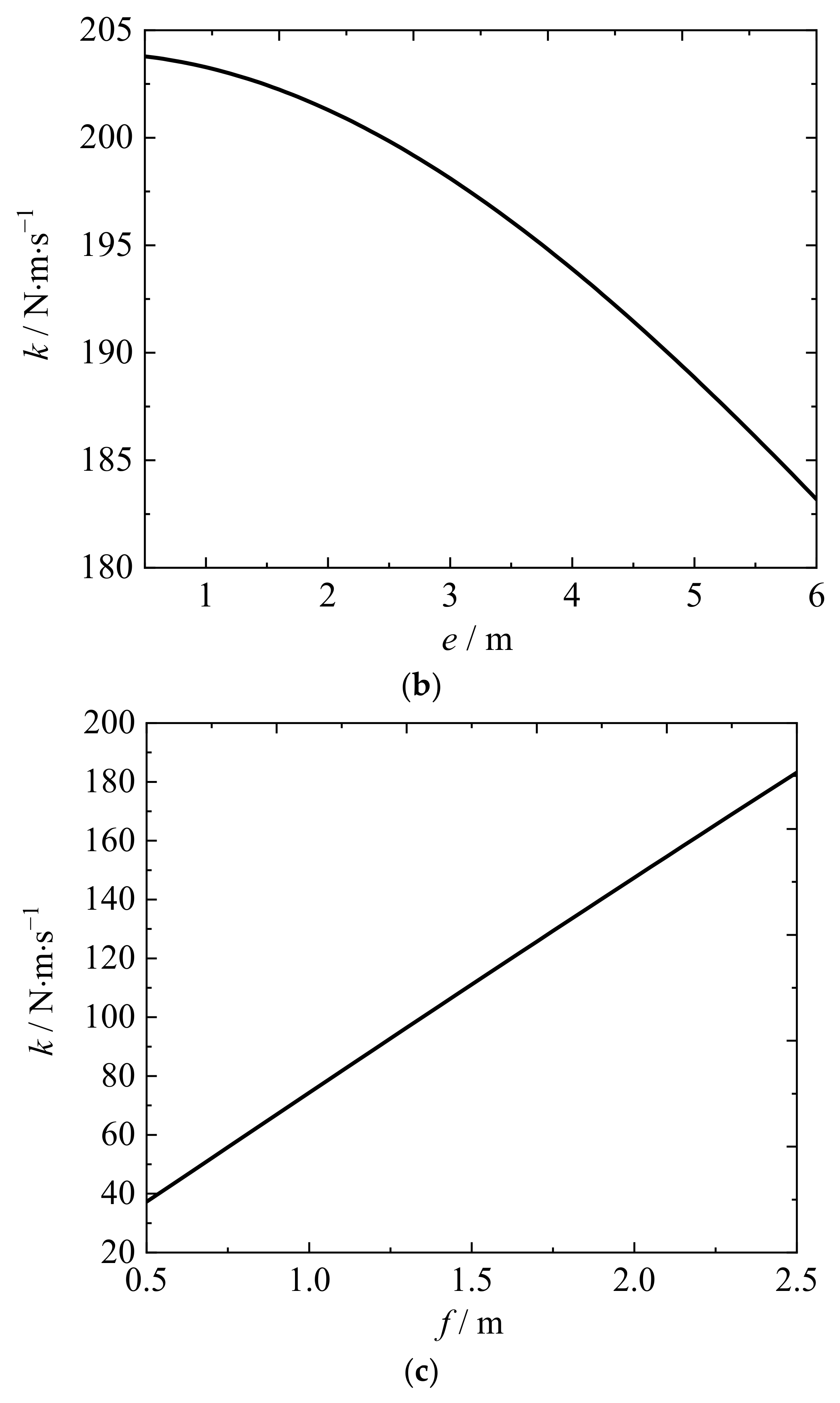
When the pressure and size of the anti-swaying hydraulic cylinders in the hydraulic system were determined, the longitudinal and transverse installation distances of the anti-swaying fixed pulleys jointly affected the structure parameter. A larger longitudinal distance and a smaller transverse distance were beneficial for increasing the structure parameter. For engineering applications, the horizontal and longitudinal distances could be selected according to size near that of a standard container;

(4)

In engineering applications, a good anti-swaying effect could be achieved by obtaining the load mass, hoisting rope length, and swaying angle speed data, then calculating the set pressure for the overflow valve of the hydraulic anti-swaying system in real-time.

References

1. Chu, F.; He, J.K.; Zheng, F.F.; Liu, M. Scheduling multiple yard cranes in two adjacent container blocks with position–dependent processing times. Comput. Ind. Eng. 2019, 136, 355–365. [Google Scholar] [CrossRef]
2. He, J.L. Berth allocation and quay crane assignment in a container terminal for the trade-off between time-saving and energy-saving. Adv. Eng. Inform. 2016, 30, 390–405. [Google Scholar] [CrossRef]
3. Sun, N.; Wu, Y.; Chen, H.; Fang, Y. An energy-optimal solution for transportation control of cranes with double pendulum dynamics: Design and experiments. Mech. Syst. Signal Process. 2018, 102, 87–101. [Google Scholar] [CrossRef]
4. Rincon, L.; Kubota, Y.; Venture, G.; Tagawa, Y. Inverse dynamic control via ‘simulation of feedback control’ by artificial neural networks for a crane system. Control Eng. Pract. 2020, 94, 104203. [Google Scholar] [CrossRef]
5. Papaioannou, V.; Pietrosanti, S.; Holderbaum, W.; Becerra, V.M. Analysis of energy usage for RTG cranes. Energy 2017, 125, 337–344. [Google Scholar] [CrossRef] [Green Version]
6. Zhong, B.; Ma, L.L.; Dong, H. Principle of optimal voltage and energy-saving for induction motor with unknown constant-torque working condition. IEEE Access 2020, 8, 187307–187316. [Google Scholar] [CrossRef]
7. Zhong, B.; Ma, L.L.; Dong, H. Research on the hoisting motor drive system’s active disturbance rejection control and energy consumption for a crane. IEEE Access 2021, 6, 94338–94351. [Google Scholar]
8. Cibicik, A.; Pedersen, E.; Egeland, O. Dynamics of luffing motion of a flexible knuckle boom crane actuated by hydraulic cylinders. Mech. Mach. Theory 2020, 143, 103616. [Google Scholar] [CrossRef]
9. McKenzie, R.A.; Irani, R.A. Motion compensation for maritime cranes during time-varying operations at the pendulum’s natural frequency. Mech. Mach. Theory 2022, 168, 104573. [Google Scholar] [CrossRef]
10. Cekus, D.; Kwiatoń, P. Effect of the rope system deformation on the working cycle of the mobile crane during interaction of wind pressure. Mech. Mach. Theory 2020, 153, 104011. [Google Scholar] [CrossRef]
11. Fatehi, M.H.; Eghtesad, M.; Amjadifard, R. Modelling and control of an overhead crane system with a flexible cable and large swing angle. J. Low Freq. Noise Vib. Act. Control. 2014, 23, 395–410. [Google Scholar] [CrossRef]
12. Sun, N.; Fang, Y.; Chen, H.; Lu, B.; Fu, Y. Slew/translation positioning and swing suppression for 4-DOF tower cranes with parametric uncertainties: Design and hardware experimentation. IEEE Trans. Ind. Electron. 2016, 63, 6407–6418. [Google Scholar] [CrossRef]
13. Drag, L. Model of an artificial neural network for optimization of payload positioning in sea waves. Ocean Eng. 2016, 115, 123–134. [Google Scholar] [CrossRef]
14. Trąbka, A. Influence of flexibilities of cranes structural components on load trajectory. J. Mech. Sci. Technol. 2016, 30, 1–14. [Google Scholar] [CrossRef]
15. Zhou, Y.; Fu, Z.K.; Zhang, J.; Li, W.F.; Gao, C.Y. A digital twin-based operation status monitoring system for port cranes. Sensors 2022, 22, 3216. [Google Scholar] [CrossRef]
16. Peláez, G.; Vaugan, J.; Izquierdo, P.; Rubio, H.; Garcła-Prada, J.C. Dynamics and embedded internet of things input shaping. Sensors 2018, 18, 1817. [Google Scholar] [CrossRef] [Green Version]
17. Zhang, M.H.; Ma, X.; Rong, X.W.; Tian, X.C.; Li, Y.B. Error tracking control for underactuated overhead cranes against arbitrary initial payload swing angles. Mech. Syst. Signal Process. 2017, 84, 268–285. [Google Scholar] [CrossRef]
18. Tuan, L.A. Fractional-order fast terminal back-stepping sliding mode control of crawler cranes. Mech. Mach. Theory 2019, 137, 297–314. [Google Scholar] [CrossRef]
19. Ismail, R.M.T.R.; That, N.D.; Ha, Q.P. Modelling and robust trajectory following for offshore container crane systems. Automat. Constr. 2000, 59, 179–187. [Google Scholar] [CrossRef]
20. Singhose, W.; Porter, L.; Kenison, M.; Kriikku, E. Effects of hoisting on the input shaping control of gantry cranes. Control Eng. Pract. 2015, 59, 1159–1165. [Google Scholar] [CrossRef]
21. Sun, N.; Fang, Y.; Chen, H.; Lu, B. Amplitude-saturated nonlinear output feedback anti-swing control for underactuated cranes with double-pendulum cargo dynamics. IEEE Trans. Ind. Electron. 2017, 64, 2135–2146. [Google Scholar] [CrossRef]
22. Cao, X.H.; Meng, C.; Zhou, Y.; Zhu, M. An improved negative zero vibration anti-swing control strategy for grab ship unloader based on elastic wire rope model. Mech. Ind. 2021, 22, 45. [Google Scholar] [CrossRef]
23. Pietrosanti, S.; Alasali, F.; Holderbaum, W. Power management system for RTG crane using fuzzy logic controller. Sustain. Energy Tech. 2020, 37, 100639. [Google Scholar] [CrossRef]
24. Liu, Z.Q.; Sun, N.; Wu, Y.M.; Xin, X.; Fang, Y.C. Nonlinear sliding mode tracking control of underactuated tower cranes. Int. J. Control Autom. 2021, 19, 1065–1077. [Google Scholar] [CrossRef]
25. Shi, H.T.; Li, G.; Ma, X.; Sun, J. Research on nonlinear coupling anti-swing control method of double pendulum gantry crane based on improved energy. Symmetry 2019, 11, 1511. [Google Scholar] [CrossRef] [Green Version]
26. Zhong, B.; Ma, L.L. Active disturbance rejection control and energy consumption of three-phase asynchronous motor based on dynamic system’s decoupling. Sustain. Energy Tech. 2021, 47, 101338. [Google Scholar] [CrossRef]
27. Zhang, Z.C.; Wu, Y.Q.; Huang, J.M. Differential-flatness-based finite-time anti-swing control of underactuated crane systems. Nonlinear Dyn. 2019, 41, 3516–3525. [Google Scholar] [CrossRef]
28. Sun, Z.; Zhao, X.J.; Sun, Z.X.; Xiang, F. Optimal sliding mode controller design based on dynamic differential evolutionary algorithm for under-actuated crane systems. IEEE Access 2018, 6, 67469–67475. [Google Scholar] [CrossRef]
29. Pezeshki, S.; Badamchizadeh, M.A.; Ghiasi, A.R.; Ghaemi, S. Control of overhead crane system using adaptive model-free and adaptive fuzzy sliding mode controllers. J. Control Autom. Electr. Syst. 2015, 26, 1–15. [Google Scholar] [CrossRef]
30. Gu, X.T.; Xu, W.M. Moving sliding mode controller for overhead cranes suffering from matched and unmatched disturbances. Trans. Ind. Meas. Control 2020, 44, 60–75. [Google Scholar] [CrossRef]
31. Zhang, M.H. Finite-time model-free trajectory tracking control for overhead cranes subject to model uncertainties, parameter variations and external disturbances. Trans. Ind. Meas. Control 2019, 41, 3516–3525. [Google Scholar] [CrossRef]
32. Chai, L.; Guo, Q.H.; Liu, H.K.; Ding, M.B. Linear active disturbance rejection control for double-pendulum overhead cranes. IEEE Access 2021, 9, 52225–52237. [Google Scholar] [CrossRef]
33. Ramli, L.; Mohamed, Z.; Jaafar, H.I. A neural network-based input shaping for swing suppression of an overhead crane under payload hoisting and mass variations. Mech. Syst. Signal Process. 2018, 107, 484–501. [Google Scholar] [CrossRef]
34. Maghsoudi, M.J.; Mohamed, Z.; Husain, A.R.; Tokhi, M.O. An optimal performance control scheme for a 3D crane. Mech. Syst. Signal Process. 2016, 666, 756–768. [Google Scholar] [CrossRef]
35. Zhang, M.; Zhang, Y.; Cheng, X. An enhanced coupling PD with sliding mode control method for underactuated double-pendulum overhead crane systems. Int. J. Control Automat. Syst. 2019, 17, 1579–1588. [Google Scholar] [CrossRef]
36. Yang, B.; Liu, Z.X.; Liu, H.K.; Li, Y.; Lin, S. A GPC-based multi-variable PID control algorithm and its application in anti-swing control and accurate positioning control for bridge cranes. Int. J. Control Autom. 2020, 18, 2522–2533. [Google Scholar] [CrossRef]
37. Sun, N.; Yang, T.; Chen, H.; Fang, Y.C.; Qian, Y.Z. Adaptive anti-swing and positioning control for 4-DOF rotary cranes subject to uncertain/unknown parameters with hardware experiments. IEEE Trans. Syst. Man Cybern. Syst. 2019, 49, 1309–1321. [Google Scholar] [CrossRef]
38. Miao, Y.B.; Xu, F.L.; Hu, Y.W.; An, J.P.; Zhang, M. Anti-swing control of the overhead crane system based on the harmony search radial basis function neural network algorithm. Adv. Mech. Eng. 2019, 11, 1687814019834458. [Google Scholar] [CrossRef] [Green Version]
39. Wu, X.Q.; He, X.X. Partial feedback linearization control for 3-D underactuated overhead crane systems. ISA Trans. 2016, 65, 361–370. [Google Scholar] [CrossRef]
40. Fu, Y.; Sun, N.; Yang, T.; Qiu, Z.H.; Fang, Y.C. Adaptive coupling anti-swing tracking control of underactuated dual boom crane systems. IEEE Trans. Syst. Man Cybern. Syst. 2021, 52, 4697–4709. [Google Scholar] [CrossRef]
41. Ramli, L.; Mohamed, Z.; Abdullahi, A.M.; Jaafar, H.I.; Lazim, I.M. Control strategies for crane systems: A comprehensive review. Mech. Syst. Signal Process. 2017, 95, 1–23. [Google Scholar] [CrossRef]
42. Li, Q.; Jia, H.; Qiu, Q.; Lu, Y.; Zhang, J.; Mao, J.; Fan, W.; Huang, M. Typhoon-induced fragility analysis of transmission tower in Ningbo area considering the effect of long-term corrosion. Appl. Sci. 2022, 12, 4774. [Google Scholar] [CrossRef]
43. Abdullahi, A.M.; Mohamed, Z.; Selamat, H.; Pota, H.R.; Abidin, M.S.Z.; Ismail, F.S.; Haruna, A. Adaptive output-based command shaping for sway control of a 3D overhead crane with payload hoisting and wind disturbance. Mech. Syst. Signal Process. 2018, 98, 157–172. [Google Scholar] [CrossRef]
44. Aktas, A.; Yazici, H.; Sever, M. LMI-based design of an I-PD+PD type LPV state feedback controller for a gantry crane. Trans. Inst. Meas. Control. 2019, 41, 1640–1655. [Google Scholar] [CrossRef]
Figure 1. The mechanical structure of the hydraulic anti-swaying system.
Applsci 12 12537 g001
Figure 2. Hydraulic principle diagram of the hydraulic anti-swaying system.
Applsci 12 12537 g002
Figure 3. Schematic diagram of the simplified structure of the crane trolley–load system.
Applsci 12 12537 g003
Figure 4. Schematic diagram of the spatial layout of the anti-swaying wire ropes.
Applsci 12 12537 g004
Figure 5. Dynamic response process for the load swaying angle. (a) k = 0. (b) k ≠ 0.
Applsci 12 12537 g005
Figure 6. Influence of k on the attenuation process of the swaying angle.
Applsci 12 12537 g006
Figure 7. Anti-swaying effect of the under-damping anti-swaying system.
Applsci 12 12537 g007
Figure 8. A pair of envelope surfaces of the under-damping anti-swaying system.
Applsci 12 12537 g008
Figure 9. Influence of the damping coefficient and the rope length on the attenuation time.
Applsci 12 12537 g009
Figure 10. Influence of the hoisting rope length on the critical-damping anti-swaying system.
Applsci 12 12537 g010
Figure 11. Anti-swaying effect of the over-damping anti-swaying system.
Applsci 12 12537 g011
Figure 12. Effects of e and f on k. (a) The joint effect of e and f on k. (b) The influence of e on k (f is constant). (c) The influence of f on k (e is constant).
Applsci 12 12537 g012aApplsci 12 12537 g012b
Publisher’s Note: MDPI stays neutral with regard to jurisdictional claims in published maps and institutional affiliations.