Abstract
To solve the problem that recommendation algorithms based on knowledge graph ignore the information of the entity itself and the user information during information aggregating, we propose a double interaction graph neural network recommendation algorithm based on knowledge graph. First, items in the dataset are selected as user-related items and then they are integrated into user features, which are enriched. Then, according to different user relationship weights and the influence weights of neighbor entities on the central entity, the graph neural network is used to integrate the features of nodes in the knowledge graph to obtain neighborhood information. Secondly, user features are interacted and aggregated with the entity’s own information and neighborhood information, respectively. Finally, the label propagation algorithm is used to train the edge weights to assist entity features learning. Experiments on two real datasets commonly used in recommended algorithms were conducted and showed that the model is better than the existing baseline models. The values of AUC and F1 on MoviesLens-1M are 0.905 and 0.835 and on the Book-Crossing are 0.698 and 0.640. Compared with the baseline model, the Precision@K index improved by 1.3–3% and the Recall@K index improved by 2.2~11.2% on the MoviesLens-1M dataset, while the Precision@K index improved by 0.6~1.6% and the Recall@K index improved by 4.5~10.8% on the Book-Crossing dataset. The model also achieves strong performance in data-sparse scenarios.
1. Introduction
Collaborative filtering (CF) [1,2] algorithm is a commonly used recommendation in recommendation systems. The algorithm has data-sparse problems [3] and cold-start problems [4,5,6], making it difficult to recommend items that are not scanned but may be of interest to users. Additional information can be introduced for CF problems. Commonly used additional information includes social networks [7], user/item attribute information [8], multimedia information (such as pictures [9], text [10], audio, video, etc.), context information [11], etc. Therefore, knowledge graph (KG) was introduced into recommendation algorithms [12,13]. The combination of KG as the additional information and recommendation system has three advantages: (1) integration of items and their attribute information and users and their attribute information into the KG, so as to capture the relationship between user and item more accurately, to explore user’s interests more deeply, and to improve more accurate personalized recommendation; (2) the entities in KG are connected by multiple relationships, which helps to provide users with recommendations; and (3) the entities in KG are connected by various relationships, and two similar items are connected through a certain relationship and recommended to users, which makes the recommendation system interpretable.
Graph embedding is to learn the structure of a graph or the adjacency relationships between nodes and transforming graph data into a low-dimensional dense vector representation. Graph embedding has problems, such as high non-linearity, preservation of structural information, and data sparsity. Methodologically, graph embedding can be divided into several types: decomposition-based method, random walk-based method, and deep learning-based method. (1) Decomposition-based method. By matrix decomposition of the matrix describing the data structure information of the graph, the nodes are transformed into a low-dimensional vector space while retaining the structural similarity. This type of method has problems, such as high time complexity and space complexity, and is not suitable for large-scale graph data. Representative model: LLE [14]. (2) Random walk-based method. The sequences generated by random walks in the graph are regarded as sentences and the nodes are regarded as words, so that the representation of nodes can be learned by analogy with word vector methods. This type of method has problems, such as the underutilization of the graph structure information and the difficulty of integrating the attribute information in the graph for representation learning. Representative models: Deepwalk [15], Node2Vec [16]. Deepwalk is a method of generating vertex embedding based on a random walk method. The random walk method of this method is completely random, for which Node2Vec is proposed. On the basis of Deepwalk, Node2Vec applies weights to random walks in the direction of DFS and BFS, so that the generated sequence can better reflect the structural information of the node. (3) Method based on deep learning. The main idea of this method is to use a graph neural network (GNN)-based method for representation learning. GNNs use a neural network to represent nodes featuring information by aggregating node neighborhood information; this method can integrate structure and attribute information for representation learning and can adapt to large-scale graphs. Representative models: GraphSAGE [17], GAT [18]. The Deepwalk method has to retrain the model to represent a new node whenever it appears. GraphSAGE can solve this problem by learning the embedding of each node in an inductive way and can use the information of known nodes to generate embeddings for unknown nodes. Each node of GraphSAGE is aggregated and represented by its neighborhood. Therefore, even if a new node appears in the graph that was not seen during the training process, it can still be represented by its neighboring nodes. GNNs did not consider the importance of different neighbor nodes when aggregating neighbor nodes. GAT introduced an attention mechanism. When calculating the representation of each node in the graph, it will assign different weights according to the different features of the neighbor nodes.
There are three methods to introduce the knowledge graph into the recommendation system. (1) Path-based method. This uses the connection information of entities in the KG for recommendation and enhances the recommendation results by the similarity between users and items. It considers KG as a heterogeneous information network, using semantic similarity in different meta-paths to refine the representation of users and items. The path-based method uses KG in a more intuitive way but relies on manual design. (2) KG Embedding. This method uses the relationships in the KG to enrich the representation of items and users requiring the use of a KG into a low-dimensional dense vector representation. Representative models: DKN [19], MKR [12]. DKN regards entity embeddings and word embeddings as different channels, then designs a CNN framework to combine together for news recommendation. The embedding-based method has high flexibility in utilizing KG to assist the recommendation system, but this method is more suitable for in-graph applications, such as knowledge graph completion, rather than recommendation. (3) A hybrid method combining knowledge graph embedding and path. The path-based method uses semantic connection information for recommendation, and the embedding-based method uses semantic representation of users or items in the KG for recommendation. Both methods only use one aspect of the information in the graph, so a hybrid method is proposed based on the idea of embedding propagation. First, the users’ preferences and interests are obtained in a transfer method on the KG, and the vector representation of user’s interest preference is performed by using graph embedding technology, and then the embedding of multi-hop neighbors of the aggregated items is used to refine the representation of items. Representative models: Ripple Network [20], KGAT [21], KGCN [22]. RippleNet trains a relationship matrix to assign weights to neighbors in the KG to propagate information, but this method has fewer sources of user information.
To address the limitations of existing methods, we propose a KGDI recommendation algorithm based on KG, which is a structure-based recommendation model that integrates KG features with the graph neural network. The core idea is that when calculating the given entity representation in KG, the weight of neighbor node aggregation depends on the relationship between them and specific users, and also depends on the influence of different neighbor nodes on the central entity, which mainly reflects the following advantages: (1) the addition of specific users can better reflect the personalized interests and improve the accuracy of the recommendation results and (2) aggregation of node feature information on the local neighborhood of the node to calculate the embedding representation of each node, which can better capture the structure of the KG.
2. Message-Passing Mechanism of Graph Neural Network
A message-passing mechanism [23] is mainly divided into two stages: (1) message aggregation, with the aggregation of the features of neighbor nodes to form a message vector, ready to be transferred to the central node and (2) message update, which combines the information of the central node with the aggregated information of the neighbor node to update the final central node representation.
The message passing of the node is shown in Figure 1, where the intermediate node refers to the target item to be predicted, , while representative Neighbors, , , etc., are first-order neighbors of , ,, etc., are second-order neighbors of , and Representative relationship represents the number of iterations. For example, if represents a film, then can be the director of the film, can be the actors of the film, etc. Suppose you want to calculate the central node , first aggregate the information passed by all first-order neighbor nodes of the central node . The neighborhood information of the central node is obtained by weighting and summing , , and their corresponding relations , , , respectively. This is then combined with the central node v’s own information to update the final representation of the central node .
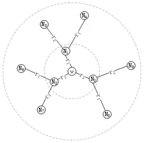
Figure 1.
Message passing between nodes.
Recently, many researchers have applied graph convolution networks to recommendation systems and achieved great success. For example, Ying et al. proposed a data efficient graph convolution (GCN) algorithm PinSage [24], which combines efficient random walk and graph convolution to generate the embedding of item nodes. For the first time, the drawing method has been applied to the industry. Embedded learning for users can also involve high-order neighborhood users who have no common interests with users. Liu et al. proposed a new interest-aware messaging GCN recommendation model (IMP-GCN) [25], in which users and their interaction items are grouped into different sub-graphs, and high-order graph convolution is performed in the sub-graphs.
3. Definition of Recommended Questions
In a typical recommendation scenario, we have a set of M users and a set of N items . Existing user–item interaction matrix . The matrix is defined according to the implicit feedback information of the user, and indicates that user interacted with item , such as scoring or purchasing. This recommendation method extracts user features based on their historical behavioral data, so it requires implicit feedback datasets.
Existing knowledge graph is a directed graph in the form of a triple , where , and denote the head entity, tail entity, and relation, where and are the set of entities and relations in the knowledge graph, respectively. For example, the triple (Farewell My Concubine, Director, Chen Kaige) means that the director of Farewell My Concubine is Chen Kaige. In many recommendation scenarios, each item corresponds to some entity on the knowledge graph, but not all entities e have items corresponding to them, so the set of items can be seen as a subset of the set of entities , i.e., .
Since the number of directly adjacent entities of each entity in the actual knowledge graph is unequal, in order to ensure that the computational dimension of each batch is fixed, we randomly sample a fixed-size number of neighbors for each entity.
The sampling process is from the inside out, as shown in Figure 2, where small circles represent entities, the central entity denotes the item whose features are to be extracted, the black entities represent entities that are sampled, the white entities represent entities that are not sampled, and represents the depth of traversal on the knowledge graph, and the sampling steps are as follows:
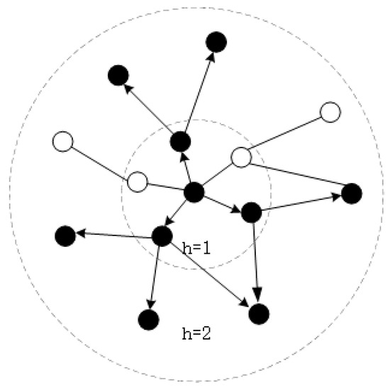
Figure 2.
The process of graph sampling.
(1) Randomly select a central node ;
(2) Find the entity set directly connected to the central node , and count the number of entities in . Compare with the size of and the number of samples : if , select k entities in (neighbors can be repeated) to form a sampled entity set ; if , select an entity without replacement in to form a sampling set.
Based on the existing user–item interaction matrix ,with the knowledge graph used as auxiliary information, the model aims to predict whether user has potential interest in item that they have not interacted with before. The ultimate goal to learn the prediction function is
where denotes the probability of user engage in item , and denotes the model parameters of the function, which mainly include entity embedding, relation embedding, weight matrix used for aggregation, and offset vector.
4. Methodology
4.1. Knowledge Graph Convolution Neural Network
Figure 3 shows the model framework of KGDI, which is divided into the embedding layer, feature integration layer, and prediction layer. Given the interaction set of user , the neighborhood set of item entity , is the neighbor entity, and the corresponding relationship between entity and , the vector representation is obtained by embedding them. The feature integration layer is divided into user feature integration and neighbor entity aggregation. User feature integration takes the concatenating vector of and embedding vectors as input for feature integration; meanwhile, user scores and neighbor entity scores the central entity and uses different scores to aggregate differently, then models the user’s interaction with item and neighbor information, respectively, and aggregates them, and finally calculates user preferences.
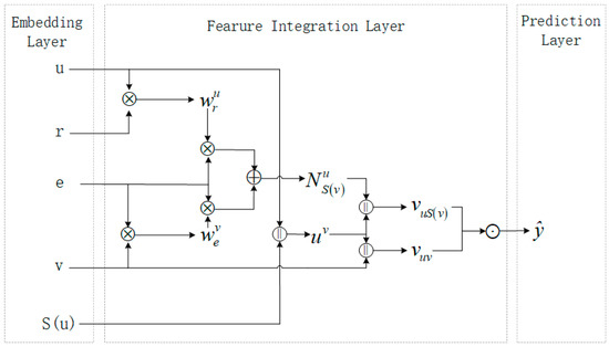
Figure 3.
KGDI model framework. denotes the element-wise inner product, denotes the element-wise summation, denotes the element-wise concatenation, and denotes the aggregation operation.
4.1.1. User Feature Integration
The items in the user–item interaction record are used as related items, and the item set is . In order to enrich the user features, the user vector and the item vector are concatenated:
where and are the weight matrix and offset vector of the network, is the mixed user features, and is the activation functions.
4.1.2. Neighbor Entity Aggregation
In the KGDI model, if the relationship vector in Figure 1 is used directly as the weight of message passing, the vector needs to be converted into a value to calculate during the calculation, which increases the difficulty of calculation. Therefore, the relation vector is converted into a weight in some way, and the weight denotes the degree of preference of different relationships influencing user behavior. For example, some users may pay more attention to movies with the same ‘star’, while some users pay more attention to movies with the same ‘genre’.
With this relation weight, users’ personalized preferences can be quantified. denotes the relation between entity and . Define the scoring function to calculate the score between a user and a relation:
where and are the feature vectors of users and relations, respectively. Because the user vector is added to every message passing, the result naturally reflects the attention of user better than taking the relation vector directly. is an inner product function that measures the user’s preference for different relationships.
Normalize the user-relation score :
Use the scoring function to calculate the influence weights of different neighbor nodes on the central entity :
Normalize the influence weights of neighbor entities on the central entity:
The embedding representation of entity is updated through the message-passing mechanism, which is mainly divided into two stages: message aggregation and message update. The iterative process of neighbor nodes feature integration is shown in Figure 4. The nodes of each layer are generated by the previous layer. In this way, the nodes of the first layer aggregate the information of the second layer. After the two-layer aggregation is completed, it can be extended to the node in layer 0, which contains all the information of the neighbors of the two layers.
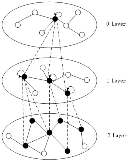
Figure 4.
Iterative process of feature fusion of neighbor nodes.
- Message aggregation
A central node has more than one neighbor, so the message aggregation function is used to aggregate the messages delivered by all neighbor nodes of node . Define the aggregate function as follows:
where is the feature of the neighbor node of entity . is not obtained directly by summing up the embedding vectors of e, but by applying different weights to and the weighted summation operation is performed between the weights and . The use of weights here reflects the idea of attention mechanism. In this way, the importance of each path is different according to the preference degree of different users when traversing the knowledge graph.
- Message update
Unlike KGCN, the presented algorithm interacts the integrated user feature with the entity and the mixed vector of the neighbor set, respectively, rather than directly integrating. This not only can effectively use the integrated item features in for one-to-one correspondence matching, but also takes into account the neighbor information.
Firstly, the vector concatenating of the user with the item and the neighbor mixed entity representation:
The final representation of the central node is updated by aggregating the concatenated entity information with the concatenated mixed neighbor entity information. In machine learning, addition works well when integrating multiple vectors. However, only linear relations can only be learned by using the additive method alone. Here, a weight matrix of dimension , an offset vector of dimension , and a nonlinear activation function are introduced. Define the message update function as follows:
There are three types of aggregator functions:
(1) GCN summation [26] aggregator (KGDI-GCN), which takes the sum of two representation vectors:
(2) GraphSAGE concat [17] aggregator (KGDI-GS), which concatenates the two presentation vectors:
(3) Bi-Interaction neighbor [21] aggregator (KGDI-BI), which interacts the entity feature with its neighbor feature . We not only learn the feature of neighbors, but also learn the feature of entities themselves. denotes that the corresponding elements in two matrices are multiplied by each other:
4.1.3. Prediction Layer
To learn the nonlinear interactions between user nodes and item nodes, this the presented algorithm uses the traditional inner product operation in matrix factorization. The calculation formula is as follows:
4.2. Label Propagation
Both the edge weights in Equation (4) are learnable and require supervised training like , and the structure of the graph also needs to be trained, which leads to the over-fitting of the model during the optimization process, resulting in poor training results. Therefore, a label propagation on edge weights is needed to assist the learning of entity representation.
The label represents the user’s rating value for the item, i.e., . The following gives the basic idea of how to predict the label of an unlabeled node using the label propagation algorithm: (1) For a given node, take the weighted average of the label values of its neighbor nodes as its own label. (2) For each unlabeled node, repeat step (1) until convergence. (3) Optimize the difference between the predicted value of the label and the true value of the label. The item label and the neighbor label have a one-to-many relationship. In order to utilize the knowledge graph information, multiple neighbor labels are fused into one label, and the relationship is used as the basis for weight assignment, as shown below:
(1) First let users rate different relationships:
(2) Aggregate the information of neighbor label :
where is the normalized user relationship scores. When obtaining neighbor label representations, neighbor information is aggregated according to these user-specific scores, where the scores between users and relations play the role of personalized filtering, that is, assigning different weights to different neighbors.
(3) Add the self-label to the aggregated neighbor labels:
(4) Label function: Use the label propagation algorithm to minimize the label function to obtain the predicted value :
Iterate over all edges; is the weight of the edge. If node has an edge, it means that the connection between the two adjacent entities is relatively strong, then the two adjacent entities have similar labels. If the edge weight of two adjacent entities is large, the constraint between them is stronger, and the labels of these two adjacent entities are more consistent.
(5) Loss function: Use the label propagation algorithm to predict the label of , obtain the predicted value label , and calculate the loss between the predicted value label and the true value label :
4.3. The Unified Loss Function
For the case of class deviation, the strategy of randomly sampling negative samples is usually used to deal with it. The design loss function formula is as follows:
In this loss function, where the first term is the binary cross-entropy, the value of represents the number of user–item pairs. The smaller the value of cross entropy is, the more accurate the model classification result. The second item is the label propagation part, which can be regarded as adding constraints to the edge weight . The last item is the regular term used to control the model parameters so as not to become excessive or large, making the training process more stable and reducing overfitting problems.
A recommendation for user is actually a mapping from item features to user item labels, i.e., , where is the feature vector of item . Therefore, Equation (21) exploits the knowledge graph structure information on the feature side and the label side to capture the user’s higher-order preferences.
4.4. Time Complexity Analysis
The time cost of the KGDI algorithm is divided into three parts. For the graph convolution part, the computational complexity of matrix multiplication at layer is ; and are the current previous transformation size, respectively. For the label propagation algorithm, its time complexity is . For the final prediction layer, only the inner product operation is performed, and the time cost of the entire training is . Finally, the overall training complexity of KGDI is . Taking the MoviesLens-1M dataset as an example, the time costs of LFM, RippleNet, KGNN-LS, KGCN, and KGDI are about 263 s, 39 min, 276 s, 304 s, and 385 s, respectively.
5. Experiments
5.1. Datasets
In order to verify the performance of the KGDI algorithm, the public datasets MovieLens-1M and Book-Crossing real datasets are compared with several similar algorithms. In order to obtain the KG corresponding to the datasets, the present work follows the preprocessing used in the MKR [12] model for the MovieLens-1M and Book-Crossing datasets. The information for the datasets is shown in Table 1.

Table 1.
Dataset information.
For each dataset, we randomly selected 80% of the interaction history of each user to constitute the training set and treated the remaining as the test set. From the training set, we randomly selected 20% of the interactions as the validation set to tune the hyper-parameters. For each observed user–item interaction, we treated it as a positive instance, and then conducted the negative sampling strategy to pair it with one negative item that the user did not previously consume.
5.2. Experimental Settings
5.2.1. Evaluation Metrics
The model was evaluated in two experimental scenarios: (1) In click-through rate (CTR) [27] prediction, the trained model was used to predict each user–item pair in the test set using AUC (probability of positives ahead of negatives) and F1 as evaluation metrics for CTR prediction. (2) In Top-K [28] recommendation, we used the trained model to select the K items with the highest predicted click probability for each user in the test set, and selected Precision@K and Recall@K to evaluate the recommendation sets.
5.2.2. Baselines
To verify the effectiveness of the KGDI model, the present work compares with the following four baselines:
LFM [29]: Uses latent features to connect users and items. The input of the model is the vector representation of each user and the vector representation of each item, and then the user’s interests and preferences are classified, and finally the items under this classification are recommended for the user.
RippleNet [20]: The user’s favorite items are as seeds, and then the seeds are spread out layer by layer on the knowledge graph to obtain the user’s vector representation. Finally, the user’s vector representation and the item’s vector representation are matrix-multiplied to obtain the interest prediction value.
KGCN [22]: Represents users with only one embedding vector, aggregating neighbor information and mixing item entities using graph convolutional network.
KGNN-LS [30]: The graph neural network architecture is applied to the knowledge graph and the user-specific relationship scoring function is used to aggregate neighborhood information with different weights. Adds label smoothing regularization to optimize KGCN. The input is also the raw features of users and items and knowledge graph.
5.2.3. Parameter Settings
The hyper-parameter settings on the datasets are shown in Table 2.
Table 2.
Hyper-parameter settings for the two datasets.
We implemented the KGDI model in python3.6, tensorflow1.13.1, and numpy1.16.6. We optimized all models with Adam optimizer. We used the default Xavier initializer to initialize the model parameters. For deep learning, the regularization coefficient and learning rate generally belong to empirical science and were set according to the empirical values of the baseline. The hyper-parameter settings for baselines were as follows. For LFM, in the MovieLens-1M dataset, the hyper-parameter was and in the Book-Crossing dataset, the hyper-parameter was . For RippleNet, in the MovieLens-1M dataset, the hyper-parameter was and in the Book-Crossing dataset, the hyper-parameter wass . For KGNN-LS, in the MovieLens-1M dataset, the hyper-parameter was and in the Book-Crossing dataset, the hyper-parameter was . The hyper-parameter settings not specified in the baseline model were the same as the default values in the experiments. For the MoviesLens-1M dataset, the embeddings size was [4096] and for the Book-Crossing dataset the embeddings size was [256].
5.3. Results and Analysis
5.3.1. Overall Comparison
The performance comparison results are presented in Table 3.
Table 3.
The results of AUC and F1 in CTR prediction.
As can be seen from Table 3, LFM is the only recommendation model that does not use knowledge graphs among all recommendation algorithms in the comparative experiments. The LFM recommendation model lagged behind other recommendation methods on all datasets in the comparative experiments. The result verifies that the introduction of knowledge graph information can promote the recommendation quality improvement of RippleNet, KGNN-LS, KGCN, and KGDI. It also proves that KGDI has passed effectiveness of knowledge graph extracting item feature vectors. On the MoviesLens-1M dataset, RippleNet performed the best among the baseline models. This indicates that RippleNet can capture user interests, especially in the case of intensive user item interactions. However, RippleNet was more sensitive to the density of the dataset, as it performed worse than KGDI on Book-Crossing. KGNN-LS performed best among all baseline models on the Book-Crossing dataset. KGNN-LS uses a graph neural network to aggregate neighborhood information, which shows that capturing neighborhood information in knowledge graph is essential for recommendation.
KGDI is always better than KGCN, because KGDI adds the influence weight of neighbor entities on the central entity when aggregating neighbor information; when aggregating entity information, the user is interacted with the item features and the aggregated neighbor features separately. This increases the information of the user and thus improves the learning of entity representation.
Figure 5 and Figure 6 show the Precision@K and Recall@K performance of Top-K recommendations for each model on the MoviesLens-1M dataset and Book-Crossing dataset, respectively.
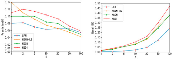
Figure 5.
MoviesLens-1M dataset on Top-K recommendation by Precision@K, Recall@K.
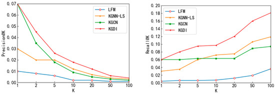
Figure 6.
Book-Crossing dataset on Top-K recommendation by Precision@K, Recall@K.
The KGDI model Recall@K performed more outstandingly on both datasets. On the MoviesLens-1M dataset, KGDI improved over the baseline model Recall@20 by 2.2~11.2%; on the Book-Crossing dataset, KGDI improved over the baseline model Recall@20 by 4.5~10.8%. In addition, the KGDI model performed better at K ≥ 20 in the MoviesLens-1M dataset. KGDI improved over the baseline model Precision@20 by 1.3~3%. The KGDI model performed better at K ≥ 10 in the Book-Crossing dataset and KGDI improved over the baseline model Precision@10 by 0.6~1.6%. Overall, although the performance of Precision@K and Recall@K was slightly lower than the baseline model in the Top-1 recommendation, this will not affect the overall performance of KGDI because KGDI performs better in other situations.
The loss control curves for training and validation and the accuracy control curves for training and validation for the MoviesLens-1M dataset and the Book-Crossing dataset are shown in Figure 7 and Figure 8.
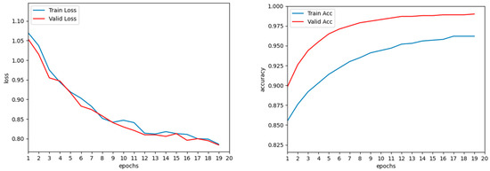
Figure 7.
Loss curve and accuracy curve of MoviesLens-1M dataset.
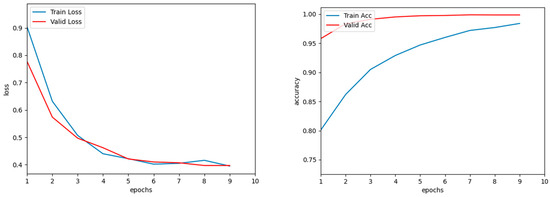
Figure 8.
Loss curve and accuracy curve of Book-Crossing dataset.
Figure 9 presents the t-SNE visualization of the embedding of the proposed structure.
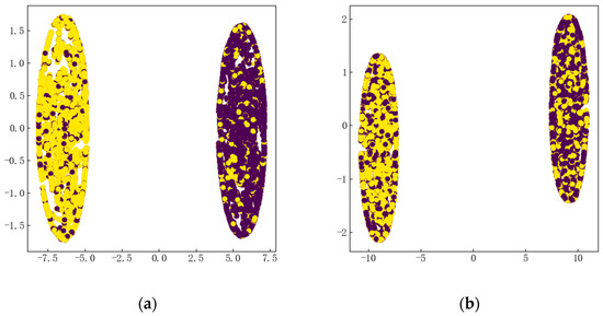
Figure 9.
Embeddings t-SNE visualization. (a) MoviesLens-1M. (b) Book-Crossing.
5.3.2. Experimental Results in Data-Sparse Scenarios
One motivation for exploiting knowledge graph is to alleviate the sparsity issue, which usually limits the expressiveness of the recommender system. In this work, under the condition that the size of the validation set and the test set are fixed, the ratio r of the full training set of MoviesLens-1M was changed from 20% to 100%, and five training sets of different sizes were used for training. Table 4 lists the five AUC values in this case.
Table 4.
AUC results of MoviesLens-1M in CTR prediction with different training set r ratios.
It can be clearly seen from the table that as the size of the training set gradually increases, its AUC value also increases. When the ratio r of the training set was 20%, the AUC values of the baseline models RippleNet and KGCN dropped by 8.3% and 9.9%, respectively, compared with the case of using the full training set, and the AUC value of KGDI only dropped by 6.4%. It shows that KGDI can still maintain good performance even in the case of sparse data.
5.3.3. Hyper-Parameters Sensitivity Analysis
The influence of the value of each hyper-parameter on the recommendation results of KGDI was studied. In the hyper-parameters tuning experiments, the remaining hyper-parameters remained the same as the table except that the selected hyper-parameters were changed.
When the embedding dimension took values of 4, 8, 16, 32, 64, and 128 the corresponding AUC values in the MoviesLens-1M and Book-Crossing datasets are shown in Table 5.
Table 5.
AUC result of KGDI with different dimension of embedding.
It can be clearly seen from the results in the figure that with the increase in the dimension, the performance of the recommender system can be improved initially because the larger dimension can learn more information contained in the dataset and knowledge graph, which encodes more information about the users and entities. If the dimension is too large, the performance of the recommender system begins to decline. This is due to the excessive dimension and will lead to the adverse effect of over-fitting during training.
When the number of neighbor sampling entities was 2, 4, 8, 16, 32, and 64 in item feature extraction the corresponding AUC values in MoviesLens-1M and Book-Crossing datasets are shown in Table 6. It can be seen from the results in the figure that when the number of neighbor sampling entities is too large, more noise will be introduced, which is not conducive to the performance of the model, thereby reducing the recommendation quality.
Table 6.
AUC result of KGDI with different neighbor sampling size K.
5.3.4. Effect of Label Propagation Algorithms
To verify the impact of the label propagation algorithm, ablation experiments were performed by disabling the label propagation algorithm. The label propagation algorithm for disabled KGDI is called KGDI-labels. The experimental results are listed in Table 7, from which it can be seen that removing the label propagation algorithm will improve the accuracy and performance of the model. The performance of KGDI-labels was lower than that of KGDI because the model has overfitting problems. It verifies the substantial influence of label propagation.
Table 7.
Effect of Label Propagation Algorithms.
6. Conclusions
In this paper, we propose an end-to-end recommendation model of the knowledge graph double interaction graph neural network, which effectively alleviates the data-sparsity problem of traditional recommendation systems. The model performs multi-hop message transmission made on the knowledge graph, which gathers the features on the central node’s neighbors to the central node. The central node feature is an integration of the multi-hop neighbor features and the central node’s own features; it concatenates the integrated user information with the entity’s own information and neighborhood information, and then conducts double interaction between the two features. Furthermore, a label propagation algorithm is proposed to learn edge weights and train transformation matrix. Experiments were conducted on the publicly available datasets MoviesLens-1M and Book-Crossing, comparing four baseline models using AUC values and F1 values as evaluation metrics, and the experiments showed that KGDI showed better results and validated the effectiveness of KGDI. There are various types of relations, and algorithms can be mined to learn the hidden states of edges to improve the performance of recommender systems. Studying interpretable recommender systems is also a promising direction.
Author Contributions
Conceptualization, S.K.; methodology, S.K. and L.S.; software, S.K.; validation, L.S.; resources, S.K.; data curation, S.K.; writing—original draft preparation, S.K.; writing—review and editing, S.K., L.S. and Z.Z. All authors have read and agreed to the published version of the manuscript.
Funding
This research was supported by the key research and development project of the Ministry of Science and Technology [No. 2017YFE0135700].
Institutional Review Board Statement
Not applicable.
Informed Consent Statement
Not applicable.
Data Availability Statement
The datasets used in this study are publicly accessible. The MoviesLens-1M dataset is available at: http://grouplens.org/datasets/movielens/, accessed on March 2003. The Book-Crossing dataset is available at: http://www2.informatik.uni-freiburg.de/~cziegler/BX/, accessed on September 2004.
Acknowledgments
We sincerely thank the editors and the reviewers for their valuable comments in improving this paper.
Conflicts of Interest
The authors declare no conflict of interest.
References
- Wang, W.; Gao, L.; Gao, Q. Collaborative filtering algorithm based on user trust and interest drift detecting. Microelectron. Comput. 2019, 36, 103–108. [Google Scholar]
- Xu, Z.; Zhao, X.; Dong, Y.; Yan, W. Video recommendation algorithm based on knowledge reasoning of knowledge graph. Comput. Eng. Des. 2020, 399, 710–715. [Google Scholar]
- Tang, J.; Chen, Y.; Zhou, M.; Wang, X. A Survey of Studies on Deep Learning Applications in POI Recommendation. Comput. Eng. 2022, 535, 12–23. [Google Scholar]
- Chen, Z.; Jiang, Y. A Personalized Recommendation Algorithm Based on Item Ratings and Attributes. Microelectron. Comput. 2011, 28, 186–189. [Google Scholar]
- Duan, D.; FU, X. Research on user cold start problem in hybrid collaborative filtering algorithm. Comput. Eng. Appl. 2017, 53, 151–156. [Google Scholar]
- Shao, Y.; Xie, Y. Research on Cold-Start Problem of Collaborative Filtering Algorithm. In Proceedings of the 2019 3rd International Conference on Big Data Research, Paris, France, 20–22 November 2019; pp. 67–71. [Google Scholar]
- Wang, H.; Zhang, F.; Hou, M.; Xie, X.; Guo, M.; Liu, Q. Shine: Signed Heterogeneous Information Network Embedding for Sentiment Link Prediction. In Proceedings of the Eleventh ACM International Conference on Web Search and Data Mining, Los Angeles, CA, USA, 5–9 February 2018; pp. 592–600. [Google Scholar]
- He, X.; Liao, L.; Zhang, H.; Nie, L.; Hu, X. Neural Collaborative Filtering. In Proceedings of the 26th International Conference on World Wide Web, Geneva, Switzerland, 3–7 April 2017; pp. 173–182. [Google Scholar]
- Zhang, F.; Yuan, N.; Lian, D.; Xie, X.; Ma, W. Collaborative Knowledge Base Embedding for Recommender Systems. In Proceedings of the 22nd ACM SIGKDD International Conference on Knowledge Discovery and Data Mining, San Francisco, CA, USA, 13–17 August 2016; pp. 353–362. [Google Scholar]
- Wang, H.; Wang, N.; Yeung, D. Collaborative Deep Learning for Recommender Systems. In Proceedings of the 21th ACM SIGKDD International Conference on Knowledge Discovery and Data Mining, Sydney, Australia, 11–14 August 2015; pp. 1235–1244. [Google Scholar]
- Hao, Z.; Liao, X.; Wen, W.; Chai, R. Collaborative Filtering Recommendation Algorithm Based on Multi-context Information. Comput. Sci. 2021, 48, 168–173. [Google Scholar]
- Wang, H.; Zhang, F.; Zhao, M.; Li, W.; Xie, X.; Guo, M. Multi-task feature learning for knowledge graph enhanced recommendation. In Proceedings of the World Wide Web Conference, San Francisco, CA, USA, 13–17 May 2019; pp. 2000–2010. [Google Scholar]
- Wang, H.; Zhang, F.; Wang, J.; Zhao, M.; Li, W.; Xie, X.; Guo, M. Exploring high-order user preference on the knowledge graph for recommender systems. ACM Trans. Inf. Syst. 2019, 37, 1–26. [Google Scholar] [CrossRef]
- Roweis, S.; Saul, L. Nonlinear dimensionality reduction by locally linear embedding. Science 2000, 290, 2323–2326. [Google Scholar] [CrossRef] [PubMed]
- Perozzi, B.; Al-Rfou, R.; Skiena, S. Deepwalk: Online Learning of Social Representations. In Proceedings of the 20th ACM SIGKDD International Conference on Knowledge Discovery and Data Mining, New York, NY, USA, 24–27 August 2014; pp. 701–710. [Google Scholar]
- Grover, A.; Leskovec, J. node2vec: Scalable Feature Learning for Networks. In Proceedings of the 22nd ACM SIGKDD International Conference on Knowledge Discovery and Data Mining, San Francisco, CA, USA, 13–17 August 2016; pp. 855–864. [Google Scholar]
- Hamiltion, W.; Ying, Z.; Leskovec, J. Inductive Representation Learning on Large Graphs. In Proceedings of the Advances in Neural Information Processing Systems 30: Annual Conference on Neural Information Processing Systems 2017, Long Beach, CA, USA, 4–9 December 2017. [Google Scholar]
- Velickovic, P.; Cucurull, G.; Casanova, A.; Romero, A.; Lio, P.; Bengio, Y. Graph Attention Networks. In Proceedings of the ICLR 2018 Conference Blind Submission, Vancouver, BC, Canada, 30 April–3 May 2018. [Google Scholar]
- Wang, H.; Zhang, F.; Xie, X.; Guo, M. DKN: Deep Knowledge-Aware Network for News Recommendation. In Proceedings of the 2018 World Wide Web Conference, Lyon, France, 23–27 April 2018; pp. 1835–1844. [Google Scholar]
- Wang, H.; Zhang, F.; Wang, J.; Zhao, M.; Li, W.; Xie, X.; Guo, M. Ripplenet: Propagating User Preferences on the Knowledge Graph for Recommender Systems. In Proceedings of the 27th ACM International Conference on Information and Knowledge Management, Torino, Italy, 22–26 October 2018; pp. 417–426. [Google Scholar]
- Wang, X.; He, X.; Cao, Y.; Liu, M.; Chua, T. Kgat: Knowledge Graph Attention Network for Recommendation. In Proceedings of the 25th ACM SIGKDD International Conference on Knowledge Discovery & Data Mining, Anchorage, AK, USA, 4–8 August 2019; pp. 950–958. [Google Scholar]
- Wang, H.; Zhao, M.; Xie, X.; Li, W.; Guo, M. Knowledge Graph Convolutional Networks for Recommender Systems. In Proceedings of the World Wide Web Conference, San Francisco, CA, USA, 13–17 May 2019; pp. 3307–3313. [Google Scholar]
- Gilmer, J.; Schoenholz, S.; Riley, P.; Vinyals, O.; Dahl, G. Neural Message Passing for Quantum Chemistry. In Proceedings of the 34th International Conference on Machine Learning, PMLR, Sydney, Australia, 6–11 August 2017; pp. 1263–1272. [Google Scholar]
- Ying, R.; He, R.; Chen, K.; Eksombatchai, P.; Hamilton, W. Graph Convolutional Neural Networks for Web-Scale Recommender Systems. In Proceedings of the 24th ACM SIGKDD International Conference on Knowledge Discovery & Data Mining, London, UK, 19–23 August 2018; pp. 974–983. [Google Scholar]
- Liu, F.; Cheng, Z.; Zhu, L.; Gao, Z.; Nie, L. Interest-Aware Message-Passing GCN for Recommendation. In Proceedings of the Web Conference 2021, Ljubljana, Slovenia, 19–23 April 2021; pp. 1296–1305. [Google Scholar]
- Kipf, T.; Welling, M. Semi-supervised classification with graph convolutional networks. In Proceedings of the 4th International Conference on Learning Representations, ICLR 2016, San Juan, Puerto Rico, 2–4 May 2016; pp. 1–14. [Google Scholar]
- Guo, H.; Tang, R.; Ye, Y.; Li, Z.; He, X.; Dong, Z. Deepfm: An end-to-end wide & deep learning framework for CTR prediction. arXiv 2018, arXiv:1804.04950. [Google Scholar]
- Li, M.; Wang, J.; Deng, H.; Liu, X. Ranking Oriented Algorithm for Top-N Recommendation. Comput. Simul. 2013, 30, 264–268. [Google Scholar]
- Chen, Y.; Liu, Z. Research on Improved Recommendation Algorithm Based on LFM Matrix Factorization. Comput. Eng. Appl. 2019, 55, 116–120+167. [Google Scholar]
- Wang, H.; Zhang, F.; Zhang, M.; Leskovec, J.; Zhao, M.; Li, W.; Wang, Z. Knowledge-aware graph neural networks with label smoothness regularization for recommender systems. In Proceedings of the 25th ACM SIGKDD International Conference on Knowledge Discovery & Data Mining, Anchorage, AK, USA, 4–8 August 2019; pp. 968–977. [Google Scholar]


Publisher’s Note: MDPI stays neutral with regard to jurisdictional claims in published maps and institutional affiliations. |
© 2022 by the authors. Licensee MDPI, Basel, Switzerland. This article is an open access article distributed under the terms and conditions of the Creative Commons Attribution (CC BY) license (https://creativecommons.org/licenses/by/4.0/).