Removal of Intra-Array Statics in Seismic Arrays Due to Variable Topography and Positioning Errors

Featured Application

The proposed corrections can be used in two different seismic applications. The first is to calculate accurate static corrections, which are applied to seismic reflection data. The second is high-resolution engineering applications.

Abstract

A receiver array is an arrangement of geophones used to enhance the signal-to-noise ratio (S/N) of seismic data. However, deviations from ideal array conditions can lead to the non-optimal performance of the array. This study investigates, quantitatively, the array performance in the presence of topographic variations and positioning errors using 2D seismic data acquired in eastern Saudi Arabia. A receiver array was laid over a sand dune with variable topography underlain by a flat sabkha that has a very shallow water table. The topographic variations and position errors were calculated from Differential Global Positioning System (D-GPS) measurements of source and receiver positions and elevations. The errors in receiver positions, measured relative to the ideal receiver spacing, gave a mean and standard deviation of about 0.35% and 1%, respectively. On the other hand, elevation errors (topographic variations) from a horizontal datum gave a mean and standard deviation of about 25% and 13%, respectively. The ideal array response was found by removing both elevation and position errors. The first-arrival energy of the array was calculated after removal of elevation and position errors separately and compared to the ideal-array energy. Comparison showed a 64% enhancement in the first-arrival energy after correcting for elevation errors alone and almost no enhancement after correcting for position errors alone. The proposed approach can be used to calculate accurate static corrections for seismic reflection processing and to generate high-resolution subsurface images for engineering applications.

1. Introduction

A seismic array is a group of seismic receivers and/or sources planted in a systematic arrangement. In general, seismic arrays are used to suppress noise in the field. Many of the existing studies on seismic arrays assume ideal array conditions with perfect element (geophone) weights, perfect implementation conditions, and simple near-surface layers. However, these assumptions are rarely satisfied in the field, hence limiting the applicability of the results of these studies to field data. In particular, it is difficult to have similar ground coupling of all array elements, leading to variable element weights. Furthermore, element spacing is practically estimated by survey crew, leading to often slightly variable element positions. Local variations in the near-surface layer, such as topography and heterogeneity, can also lead to more non-ideal array conditions. All these conditions may decrease the effectiveness of the array’s multi-channel processing and its waveform [1]. Originally, seismic arrays were developed to monitor nuclear explosions [2]. The studies of nuclear explosion identification have been employed to distinguish between a natural earthquake and nuclear explosion [3,4]. Ref. [5] shows that seismic arrays improve the velocity models of the Earth’s interior using large-number and dense spatial sampling of the seismic wavefield at several locations on the Earth’s surface. More recently, seismic arrays have been implemented in high-resolution imaging [6,7], shallow geology applications [8,9,10], monitoring induced seismicity [11], seismic imaging using ambient seismic noise [12], and seismic signal processing using distributed acoustic sensing (DAS) [13]. Ref. [14] proposed an efficient algorithm for ambient seismic noise beamforming without the need for explicit cross-correlations, while [15] presented a case study using a 10-month ambient DAS data set acquired on a fiber array to investigate long-term seasonal velocity variations. Seismic arrays are often integrated with other geophysical methods for a better understanding of the subsurface conditions [10,16,17,18]

In terms of reflection seismology, the main purpose of an array of geophones is to increase the signal-to-noise ratio (S/N) by enhancing the desired signals (reflections) and attenuating seismic noise during the acquisition of seismic data in the field. As the desired seismic signals (reflections) travel across the array with a much higher horizontal velocity, the signals produce a longer wavelength, as compared to that of the unwanted signals [19]. The desired signals are usually those that have been reflected from deep geologic horizons approaching the array at almost normal incidence. The unwanted signals are incoherent noise or horizontally traveling ground roll. Thus, a geophone array can also be considered as a directional filter [20].

Seismic array response is the arithmetic sum of traces recorded by geophones (elements) in the array. Ref. [21] presented general concepts of arrays, where they used harmonic analysis to explain the array response disrupted by variations in velocity, dip, and elevation within the array length. Ref. [22] described a method for computing the expected waveform from a closely spaced array of shots or geophones when the individual signal is a pulse and studied the effects of various array weighting functions on the performance of seismic arrays. Ref. [23] presented a study on the effects of errors in position and weighting on the array response, where they used plane harmonic waves with different weights. Ref. [24] investigated effects of errors in gain and position on the array response. Ref. [25] explained the wavelet response due to errors in weights and positions of the elements of the geophone arrays with respect to several variables. These variables included the error amount, number of array elements, and weighting function. They found that the degradation of the wavelet response increased nonlinearly with the error’s value, number of elements, and weighting function complexity. A similar case was investigated by [26], wherein they evaluated the effects on the array response caused by topographic variations (i.e., deviations from the datum) within receiver arrays. They found that these variations had more negative effects on the array response than position errors because of their relatively high error amount in most environments. In addition, topographic variations directly affect the vertically traveling signals as opposed to position errors, which mainly affect noise. Finally, topographic variations leave very little human control to reduce their amount, whereas position errors can be reduced using more accurate instruments and measurement procedures.

Ref. [27] studied the performance of an array in the presence of lateral near-surface heterogeneities. They used a model with two adjacent layers to study the array performance as a function of the number of affected elements and the velocity ratio between the two adjacent layers. They found that the array performance decreased with the number of affected elements and amount of deviation of the velocity ratio from unity. Ref. [28] studied the change in the wavelet response of seismic receiver arrays in the presence of a dipping near-surface layer. They used a model with different dip and incidence angles as well as various types of signal and noise incident on the array. Their results show that incidence and dip angles have opposite effects on the array response. Refs. [29,30] studied the array response in the presence of laterally varying thickness of the weathering layer. They generated several models and calculated their corresponding array responses in the ideal and perturbed cases. They found that horizontally traveling waves were less affected than vertically traveling waves in all studied models and errors. Ref. [31] studied the seismic array response in the presence of variations in elements’ elevations, positions, and weights using a zero-phase Ricker wavelet. They found that topography had the largest effects on the array response and that different error types did not combine linearly.

Almost all previous studies have addressed the effects of non-ideal array conditions using analytical (or numerical) modeling approaches without testing their approaches on field data. The problem with field data studies is the difficulty in measuring the exact position and elevation of all receivers. In this paper, we summarize, modify, and update equations required for correcting non-ideal array conditions; then, we study the array response in the presence of topographic variations (i.e., elevation errors) and positioning errors within the array using field data from a shallow seismic survey acquired in eastern Saudi Arabia. We quantify the elevation and position errors (relative to a datum and nominal geophone spacing, respectively) at every geophone location using their Differential Global Positioning System (D-GPS) coordinates. Furthermore, we quantify enhancements in the array response using the stacked energy of first arrivals in each error case normalized by its corresponding error-free case.

This paper starts with the calculation of the velocities of the direct and refraction events in the presence of elevation and position errors. Next, the elevation and position errors are calculated using the survey geometry information. This is followed by calculation of the array response in terms of its trace energy after elevation error removal, position error removal, and removal of both errors. We finally compare them with the trace response of the ideal case (i.e., after removing both elevation and position errors).

2. Methodology

2.1. Direct Event

The direct P-wave can be defined as the P-wave that travels through the ground surface directly from the source to the receiver. To calculate the velocity ($V_1$) of the incidence (uppermost) medium, Equation (1) is used [32]:

$$T_d=\frac{X}{V_1},$$

(1)

where $T_d$ is the arrival travel time of the direct wave to a receiver at offset X. The arrival travel times of the direct wave are picked (estimated) from the traces (records), while offsets X are given by the survey geometry information.

2.2. Refraction Event

The head wave is generated when the velocity of the refraction medium ($V_2$) is larger than that of the incidence medium and the incidence angle is equal to the critical angle ${\theta }_c$. Here, the transmitted wave travels just below and parallel to the interface. To find the velocity of the refraction medium, the following time–distance equation is used:

$$T_h=\frac{X}{V_2}+\frac{2H\cos {\theta }_c}{V_1},$$

(2)

where $T_h$ is the arrival traveltime of the head wave at offset $X$ and H is the thickness of the uppermost layer. Equation (2) describes a straight line relating $T_h$ and $X$ with an intercept of $2H\cos {\theta }_c/V_1$ and a slope of $1/V_2$. The refraction velocity in this case can be calculated by finding the inverse of the slope of the best-fit line to the $T_h-X$ plot of the head wave. In general, when a wave encounters an interface between two media, Snell’s law is used to relate incident and transmitted angles [32]:

$$\frac{\sin {\theta }_1}{V_1}=\frac{\sin {\theta }_2}{V_2},$$

(3)

where ${\theta }_1$ and ${\theta }_2$ are the ray incident and transmitted angles in the upper ($V_1)$ and lower ($V_2$) media, respectively. The critical angle ${\theta }_c$ takes place when ${\theta }_2={90}^{\mathrm{o}}$, which can be calculated as:

$${\theta }_c={\sin }^{-1}\left(\frac{V_1}{V_2}\right),$$

(4)

In the case of a dipping refractor, the critical angle ${\theta }_c$ can be calculated from the apparent refractor velocities in the up-dip ($V_{2u}$) and down-dip ($V_{2d}$) directions using Equation (5) [32]:

$${\theta }_c=\frac{1}{2}\left[{\sin }^{-1}\left(\frac{V_1}{V_{2d}}\right)+{\sin }^{-1}\left(\frac{V_1}{V_{2u}}\right)\right],$$

(5)

The apparent refractor velocities can be determined by picking arrival travel times from shots in the up-dip and down-dip sides. Once ${\theta }_c$ is calculated, the refractor medium velocity $V_2$ can be determined as [32]:

$$V_2=\frac{V_1}{\sin {\theta }_c},$$

(6)

2.3. Position and Elevation Error

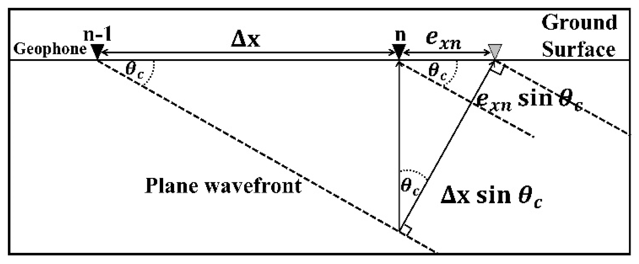
2.3.1. Position Error

Ideally, there is a desirably fixed nominal spacing between successive receivers, which we call the ideal position (spacing) $\Delta X$. However, in practice, receiver spacing might differ from the ideal spacing due to field conditions and human errors (Figure 1). The actual receiver spacing at the nth receiver ($\Delta X_{cn}$) can be calculated from D-GPS measurements acquired in the field as follows:

$$\Delta X_{cn}=\sqrt{{\left(x_n-x_{n-1}\right)}^2+{\left(y_n-y_{n-1}\right)}^2 },$$

(7)

where $x_n$ and $x_{n-1}$ are the D-GPS Easting and $y_n$ and $y_{n-1}$ are the Northing values of the nth receiver and its neighbor closer to the source. To calculate the position’s error at the nth receiver, Equation (8) is used:

$$e_{xn}=\Delta X-\Delta X_{cn} ,$$

(8)

which is the difference between the ideal and calculated positions of the nth receiver.

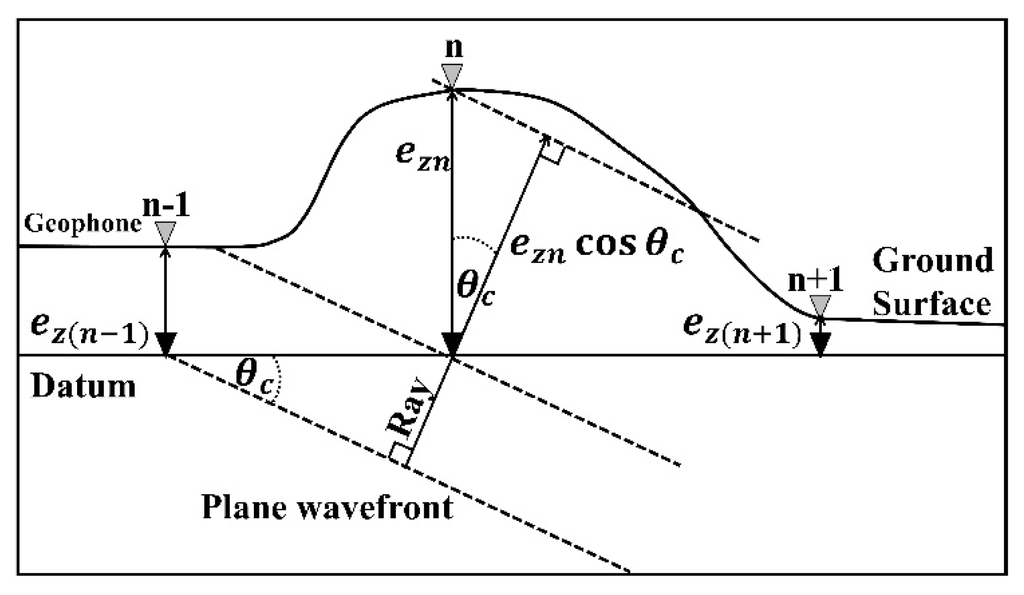
2.3.2. Elevation Error

Recording seismic data at sites with rough terrain or big elevation differences (Figure 2) is challenging. The big difference in elevation affects the data results, particularly regarding accurate travel time picking. To overcome this problem, we first calculate the elevation error, then remove it from the recorded data. Equation (9) is used to calculate the elevation error of the nth receiver:

$$e_{zn}=Z_n-Z_D,$$

(9)

where $Z_n$ and $Z_D$ are the elevations of the nth receiver and the datum (reference plane), respectively, from mean sea level, and are available from the D-GPS measurements.

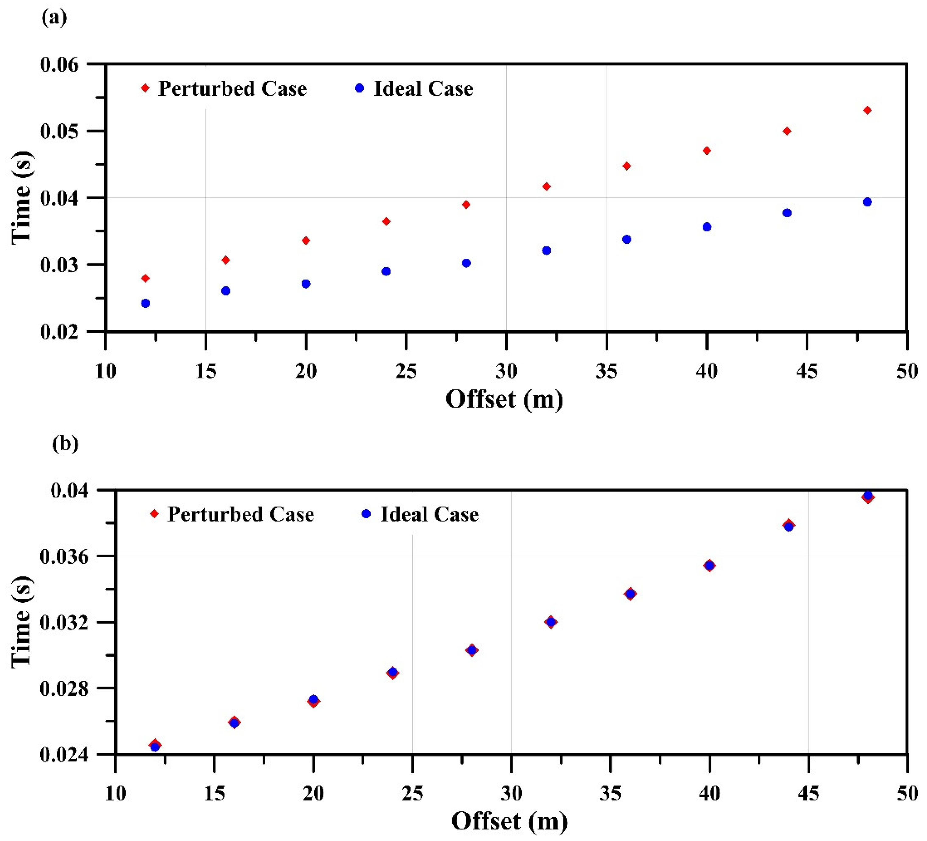
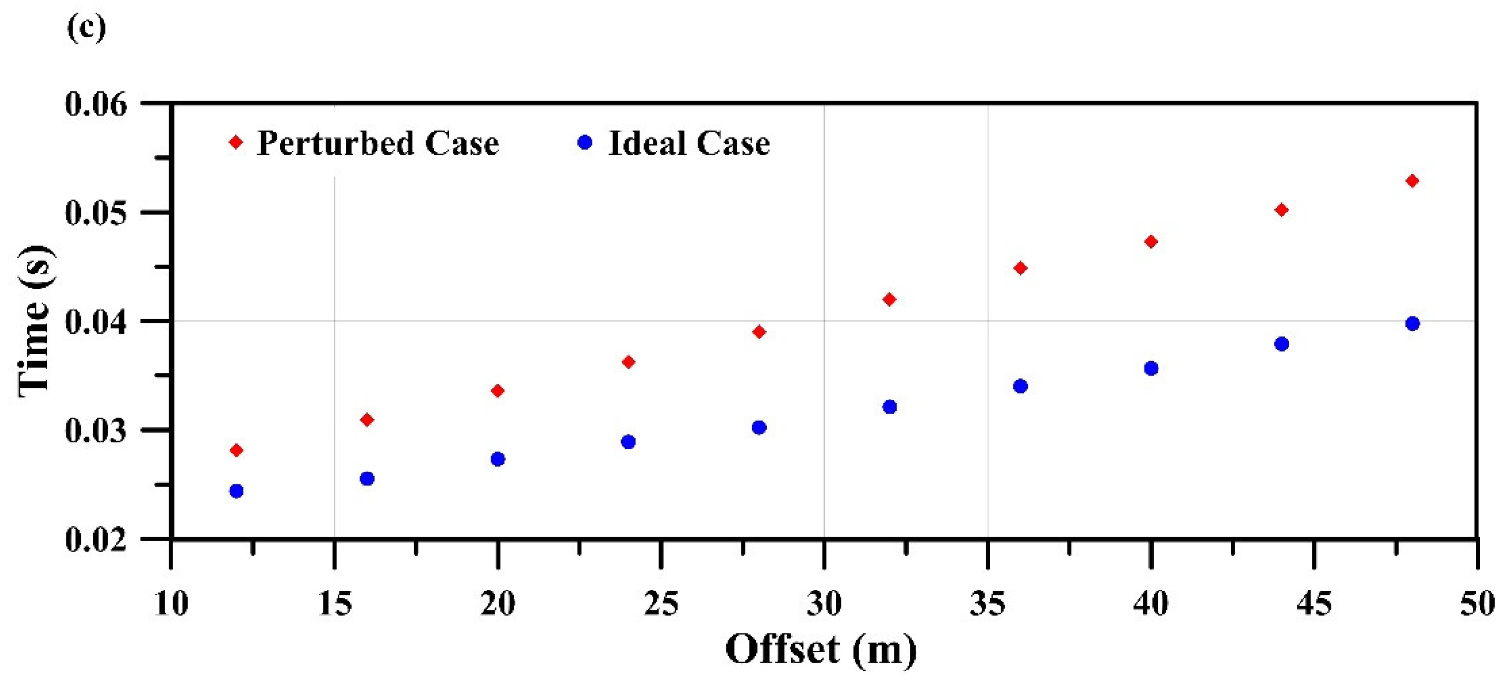
2.4. Traveltimes for Ideal and Error Cases

2.4.1. Perturbed Case

The perturbed case is defined in this study as the raw data acquired in the field without applying any time corrections. The travel time of the nth receiver for the perturbed case ($T_n$) is the picked first arrival traveltime with no elevation and/or position corrections.

2.4.2. Position’s Error Removal

The travel time difference due to position error ($\Delta T{e}_{xn}$) is the travel time of the nth receiver calculated using Equation (10):

$$\Delta T{e}_{xn}=\frac{e_{xn}\sin {\theta }_c}{V_1},$$

(10)

To calculate the first arrival travel time of the nth receiver for the position removal error case ($T_{xn}$), $\Delta T{e}_{xn}$ must be removed from the perturbed case traveltime ($T_n$) as follows:

$$T_{xn}=T_n-\Delta T{e}_{xn}$$

(11)

2.4.3. Elevation Error Removal

The travel time difference due to the elevation error ($\Delta T{e}_{zn}$) of the nth receiver is calculated using Equation (12):

$$\Delta T{e}_{zn}=\frac{e_{zn}\cos {\theta }_c}{V_1},$$

(12)

Similar to the travel time calculation of the position error removal case, the first arrival travel time of the elevation’s error removal case ($T_{zn}$) can be calculated by removing $\Delta T{e}_{zn}$ from the perturbed case traveltime $T_n$ using Equation (13):

$$T_{zn}=T_n-\Delta T{e}_{zn}$$

(13)

2.4.4. Ideal Case

The ideal case can be defined as the case after applying both position and elevation corrections on the raw data acquired in the field. The first arrival travel time of the ideal case for the nth receiver ($T_{cn}$) can be calculated from the perturbed case travel time using Equation (14):

$$T_{cn}=T_n-\left(\Delta T{e}_{xn}+\Delta T{e}_{zn}\right),$$

(14)

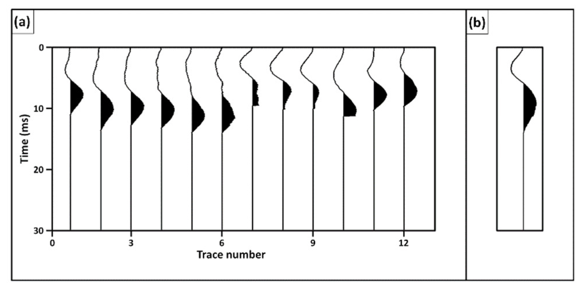
2.5. Wavelet Response and Trace Energy

To calculate the trace energy in the first arrival event, the following steps are followed:

• Window the first wavelet of the first arrival head-wave event while maintaining the timing information ($T_n$) of the first arrival on each trace.
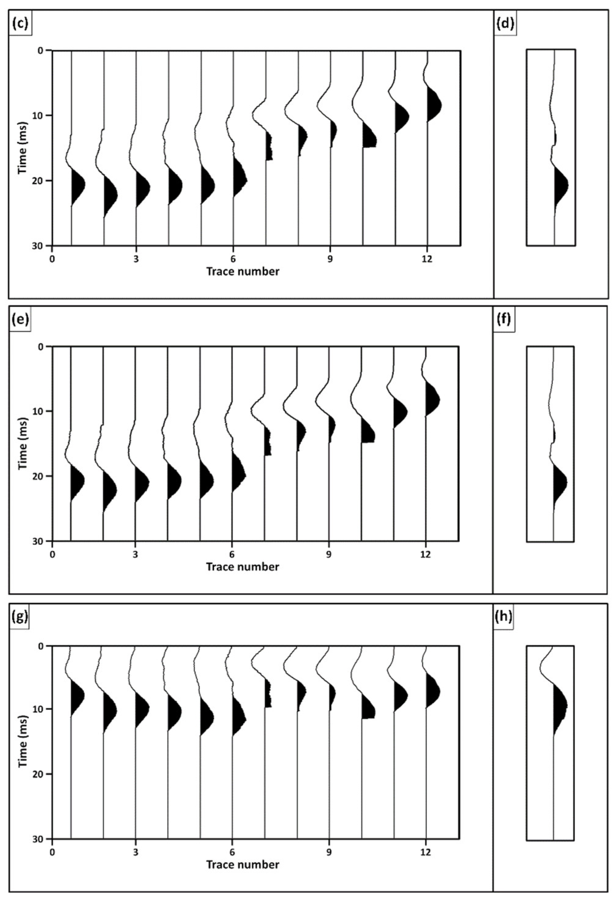
• Shift each nth windowed trace such that its first sample is at $t=0$. This produces the ideal trace wavelet response ($G_{cn}\left(t\right)$). Sum $G_{cn}\left(t\right)$ across $n$ to produce the ideal array response ($G_c\left(t\right)$) and calculate its corresponding array trace energy ($E_c$) as follows:

  $$E_c={\displaystyle \sum }_{m=1}^M{G}_{cm}^2\left(t\right),$$

  (15)

  where $M$ is the number of samples in $G_c\left(t\right)$.
• Shift each $G_{cn}\left(t\right)$ by its corresponding $\Delta T{e}_{xn}$ to produce the trace wavelet response with position errors only ($G_{xn}\left(t\right)$). Sum $G_{xn}\left(t\right)$ across n to produce the array response with position errors only ($G_x\left(t\right)$) and calculate its corresponding array trace energy (E_x) as follows:

  $$E_x={\displaystyle \sum }_{m=1}^M{G}_{xm}^2\left(t\right),$$

  (16)

The decibel (dB)-scaled normalized array energy with position errors only $E_{Nx}^{\prime }\left(dB\right)$ is calculated as follows:

$$E_{Nx}^{\prime }\left(dB\right)=20{\log }_{10}{E}_{Nx},$$

(17)

where $E_{Nx}$ is the normalized array trace energy with position errors only defined as:

$$E_{Nx}=\frac{E_x}{E_c},$$

(18)

4.

Starting with $G_{cn}\left(t\right)$ again, shift each $G_{cn}\left(t\right)$ by its corresponding $\Delta T{e}_{zn}$ to produce the trace wavelet response with elevation errors only ($G_{zn}\left(t\right)$). Sum $G_{zn}\left(t\right)$ across n to produce the array response with elevation errors only ($Gz\left(t\right)$) and calculate its corresponding array trace energy ($E_z$) as follows:

$$E_Z={\displaystyle \sum }_{m=1}^M{G}_{Zm}^2\left(t\right),$$

(19)

The dB-scaled normalized array energy with elevation errors only $E_{NZ}^{\prime }\left(dB\right)$ is calculated as follows:

$$E_{NZ}^{\prime }\left(dB\right)=20{\log }_{10}{E}_{NZ},$$

(20)

where $E_{Nz}$ is the normalized array trace energy with elevation errors only defined as:

$$E_{NZ}=\frac{E_Z}{E_c},$$

(21)

5.

Starting with $G_{cn}\left(t\right)$ again, shift each $G_{cn}\left(t\right)$ by its corresponding ($\Delta T{e}_{xn}+\Delta T{e}_{zn}$) to produce the perturbed wavelet response of the trace with combined position and elevation errors ($G_{xzn}\left(t\right)$). Sum $G_{xzn}\left(t\right)$ across n to produce the array response with both position and elevation errors ($G_{xz}\left(t\right)$) and calculate its corresponding array trace energy ($E_{xz}$) as follows:

$$E_{xZ}={\displaystyle \sum }_{m=1}^M{G}_{xZm}^2\left(t\right),$$

(22)

The dB-scaled normalized array trace energy for the perturbed case $E_{NxZ}^{\prime }\left(dB\right)$ is calculated as follows:

$${E^{\prime }}_{NxZ}\left(dB\right)=20{\log }_{10}{E}_{NxZ},$$

(23)

where $E_{Nxz}$ is the normalized array trace energy for the perturbed case defined as:

$$E_{NxZ}=\frac{E_{xZ}}{E_c},$$

(24)

3. Results and Discussion

3.1. Geological Setting

The field data were recorded over a barchan dune near Dammam city (26°20′57.2″ N 49°49′51.4″ E), Saudi Arabia (Figure 3a,b). The thickness of the dune ranges from 0 to 7 m and it overlays a flat Sabkha layer. One borehole was drilled up to 10 m deep at the midslope of the dune, and was used as ground truth and for result confirmation. A complete core was extracted from the top 3.5 m, then a core sample of only 0.7 m was extracted at each 1.5 m depth range. The well penetrated the entire dune, as well as the top 3 m of the underlying sabkha.

Based on the samples extracted from the borehole, the dominant mineral in the dune is quartz. We also found small amounts of feldspar and traces of calcite. The sabkha layer contains quartz, feldspar, calcite, and significant amounts of halite and gypsum. The top 2.5 m of the sabkha was composed of fine-grained to medium-grained sand, while the bottom 0.5 m contained muddy sand with a noticeable fraction of fine grains. Sediments in the top 7.6 m of the drilled interval showed partial saturation, whereas the bottom 2.4 m was fully water saturated.

3.2. Data Acquisition

We demonstrate our methodology using a shallow seismic survey acquired in eastern Saudi Arabia (Figure 3a) at the approximate GPS coordinates (26.351575 N, 49.829184 E). Figure 3b shows the survey location where the geological setting was a sand dune over Sabkha. The acquired data consisted of a 2D seismic line with 24 vertical receivers having a nominal spacing of 4 m. Five shots were produced by a 10 kg sledgehammer located at offsets of −4, 0, 46, 92, and 96 m, where the first receiver was placed at offset 0 m. Positions and elevations of all receiver and shot points were measured using D-GPS.

3.3. Data Analysis

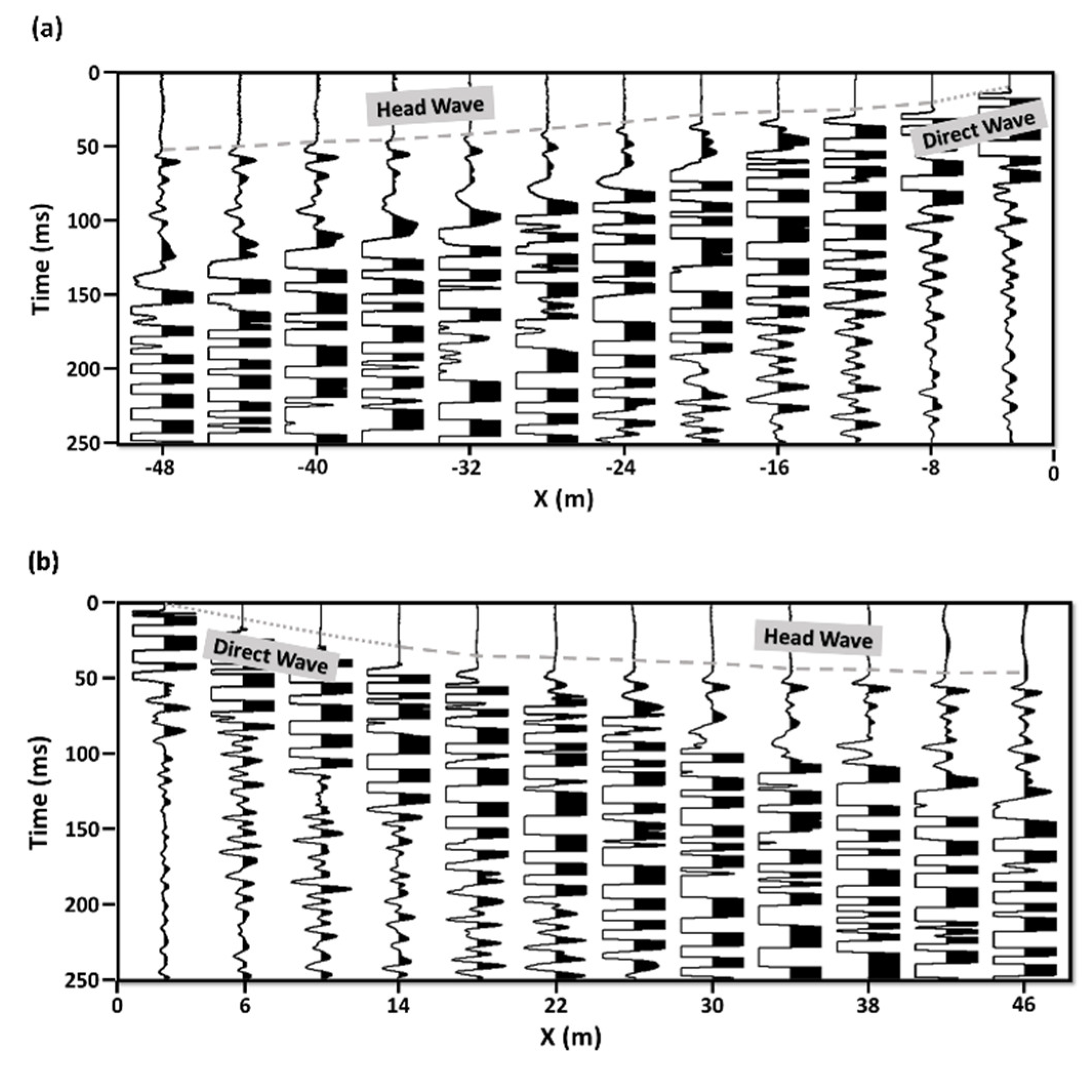
3.3.1. First Arrival Picking

For illustration purposes, we applied the proposed method to the 12 receivers between shots 1 and 3 (Figure 3b,c). Far-offset receivers were not used because the signal became too weak to pick confidently. Figure 4 shows the first and third shot gathers of the real data set. Arrival travel times were picked manually for both direct and head waves. For the direct wave, the first arrival travel time was picked only on the two receivers closest to the source since direct waves were observed only on these traces. The first picked arrival travel times of the direct wave from all shots are shown in

Table 1. First arrival travel times of direct wave and corresponding offsets and velocities from all shots of the survey. The two traces from shot gather 3 (marked by *) have been excluded from averaging because they were considered outliers.

Shot Gather No.	Trace No	Offset (m)	First Arrival Time (s)	$\mathbf{Velocity} {\mathit{V}}_1 (\mathbf{m}/\mathbf{s})$
Shot Gather 1	Trace 1	4	0.013	311
	Trace 2	8	0.025	323
Shot Gather 2	Trace 2	4	0.013	299
	Trace 3	8	0.026	320
Shot Gather 3 (left)	Trace 1 *	2	0.004	500
	Trace 2	6	0.015	349
Shot Gather 3 (right)	Trace 1 *	2	0.005	400
	Trace 2	6	0.016	344
Shot Gather 4	Trace 2	4	0.013	314
	Trace 3	8	0.027	283
Shot Gather 5	Trace 1	4	0.013	299
	Trace 2	8	0.027	286
Average velocity V1 (m/s)	313

, whereas the picks of the head wave from the down-dip (shot 1) and up-dip (shot 3) are shown in

Table 2. First arrival travel times of the head wave from shot gather 1 and 3 with the values of ground-surface dip angle ($\alpha$), critical angle (${\theta }_c$) and refraction medium velocity ($V_2$).

Trace Number	Shot Gather 1 (Down-dip)		Shot Gather 3 (Up-dip)
	Offset (m)	First Arrival Time (s)	Offset (m)	First Arrival Time (s)
13	48	0.053	2	0.004
14	44	0.050	6	0.015
15	40	0.047	10	0.027
16	36	0.045	14	0.039
17	32	0.042	18	0.043
18	28	0.039	22	0.044
19	24	0.036	26	0.045
20	20	0.034	30	0.046
21	16	0.031	34	0.047
22	12	0.028	38	0.048
23	8	0.026	42	0.049
24	4	0.012	46	0.052
$\alpha$ (deg)		3.2
${\theta }_c$ (deg)		9.2
$\mathrm{Apparent} \mathrm{velocities} V_u$$\mathrm{and} V_d$ (m/s)		1455		2967
$\mathrm{True} \mathrm{refraction} \mathrm{medium} \mathrm{velocity} V_2$ (m/s)		1949

.

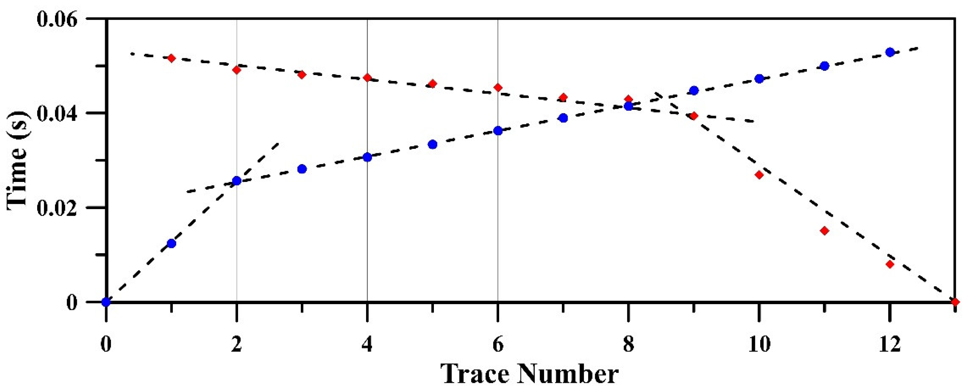
3.3.2. Velocity Calculation

The average dune velocity is $V_1=313 \mathrm{m}/\mathrm{s}$, calculated from the direct-wave velocities in the five shot records (Table 1). Head-wave velocities $V_2$ are calculated from the slopes of the best-fit lines to the first arrival traveltimes of the up-dip and down-dip directions (Figure 5). The critical angle and true head-wave velocity are calculated by Equations (5) and (6) to be ${\theta }_c={9.2}^{°}$ and $V_2=1949 \mathrm{m}/\mathrm{s}$, respectively (Table 2).

3.3.3. Error Calculation

To calculate position errors in the study area, Equation (8) is used, where the ideal spacing $\Delta X=4$ m is assumed and the calculated spacing $\Delta X_{cn}$ is measured from D-GPS Easting and Northing coordinates for each receiver (

Table 3. Measured position coordinates using D-GPS and position errors of the 12 studied traces. Position errors are measured with respect to the ideal spacing of 4 m giving a relative mean and standard deviation of about 0.35% and 1%, respectively.

Trace	$\mathit{X}$ (m)	$\mathit{Y}$ (m)	Calculated Distance (m)	${\mathit{e}}_{\mathit{x}\mathit{n}} \left(\mathbf{m}\right)$
Reference position	2,915,129	383,141
13	2,915,126	383,189	3.995	−0.005
14	2,915,126	383,185	3.945	−0.055
15	2,915,127	383,181	4.035	0.035
16	2,915,127	383,177	3.939	−0.061
17	2,915,127	383,173	4.025	0.025
18	2,915,127	383,169	3.972	−0.028
19	2,915,127	383,165	3.985	−0.015
20	2,915,127	383,161	3.938	−0.062
21	2,915,128	383,157	4.022	0.022
22	2,915,128	383,153	3.940	−0.060
23	2,915,128	383,149	3.986	−0.014
24	2,915,128	383,145	4.056	0.056
Minimum position error (m)				−0.062
Maximum position error (m)				0.056
Mean position error (m)				−0.014
Median position error (m)				−0.015
Standard deviation of position errors (m)				0.041

). Results of the position errors show that the mean and standard deviation of the errors are 0.014 and 0.041 m (0.35% and 1.025% of ideal spacing), respectively, which are negligible. Moreover, Equation (9) is used to calculate the elevation errors where a horizontal datum is chosen at the first shot elevation (i.e., datum = 9.4 m above mean sea level). Elevation errors are shown in

Table 4. Elevation values and errors of the 12 studied traces. Errors are measured with respect to the datum elevation at 9.41 m giving a relative mean and standard deviation of about 25% and 13%, respectively.

Trace	$\mathit{X}$ (m)	$\mathit{Y}$ (m)	Elevation Z (m)	${\mathit{e}}_{\mathit{z}\mathit{n}} \left(\mathbf{m}\right)$
Reference position	2,915,129	383,141	9.41
13	2,915,126	383,189	13.44	4.03
14	2,915,126	383,185	13.19	3.78
15	2,915,127	383,181	12.97	3.56
16	2,915,127	383,177	12.70	3.29
17	2,915,127	383,173	12.41	3.00
18	2,915,127	383,169	12.08	2.67
19	2,915,127	383,165	11.68	2.27
20	2,915,127	383,161	11.32	1.91
21	2,915,128	383,157	10.90	1.50
22	2,915,128	383,153	10.52	1.11
23	2,915,128	383,149	10.19	0.78
24	2,915,128	383,145	9.81	0.40
Minimum elevation error (m)				0.40
Maximum elevation error (m)				4.03
Mean elevation error (m)				2.36
Median elevation error (m)				2.47
Standard deviation of elevation errors (m)				1.22

. In comparison to position errors, elevation errors have a mean and standard deviation of 2.36 and 1.22 m (25.1% and 13% relative to the datum elevation), respectively, which are relatively considerable. Therefore, it is expected that most effects on the seismic array response are attributed to elevation errors in this case. The first arrival travel times of the perturbed and ideal cases are shown in Figure 6a.

3.3.4. Responses Calculation

After calculating the position and elevation errors, we calculate the array responses in various cases using the procedure described in Section 2.4 above. The ideal trace wavelet responses ($G_{cn}\left(t\right)$) are shown in Figure 7a and their corresponding array wavelet response ($G_c\left(t\right)$) is shown in Figure 7b. The array trace energy for the ideal case (i.e., after removal of both position and elevation errors) is $E_c=2237$. The perturbed trace wavelet responses ($G_{xzn}\left(t\right)$) are shown in Figure 7c and their corresponding array wavelet response ($G_{xz}\left(t\right)$) is shown in Figure 7d. The array trace energy for the perturbed case is $E_{xz}=797$. The normalized array trace energy of the perturbed case is calculated using Equation (23) to be $E_{Nxz}^{\prime }=-9 \mathrm{dB}$. These results demonstrate the considerable amount of degradation in the array trace energy due to position and elevation errors in this survey.

To understand the separate effects of position and elevation errors on the seismic array response, the first arrival travel times after separately removing each of these errors is calculated. Starting with elevation error removal, Equation (13) is used to calculate the first arrival travel time for this case. Comparison between the travel times of the ideal case and the elevation error removal case shows that elevation errors have large contributions in all picked head-wave first arrival travel times (Figure 6b). Figure 7e shows the trace wavelet responses after application of elevation errors to the ideal trace responses ($G_{zn}\left(t\right)$) and Figure 7f shows the corresponding array response ($G_z\left(t\right)$). Now, the array trace energy is calculated to be $E_z=795$, which is much smaller than the array trace energy of the ideal case (i.e., $E_c=2237$). The normalized array trace energy is $E_{Nz}^{\prime }=-9 \mathrm{dB}$, which is similar to that in the perturbed case, indicating that most degradation is attributed to elevation errors.

The same steps are carried out for the removal of only the position errors using Equation (11) and, hence, update the first arrival travel times. Figure 6c shows a comparison of the head-wave travel times between the ideal and position error removal cases. This comparison indicates that position errors have a very small effect on the first arrival travel times. The trace wavelet responses after position error removal and their corresponding array response are shown in Figure 7g,h, respectively. The array trace energy after the removal of only position errors is calculated to be $E_x=2237$, which is almost equal to that of the ideal case, leading to a normalized array trace energy $E_{Nx}^{\prime }=0 \mathrm{dB}$. Similar results were also reported by previous studies [30,31], as discussed in the next section.

3.3.5. Comparison with Previous Studies

We compare our results to those expected by [31] by applying their method to calculate array trace responses involving position errors only, elevation errors only, and combined position and elevation errors using the parameters of our data. The head-wave arrival in our data has a dominant frequency of 65 Hz and is incident at ${9.2}^{°}$ on a 12-element array that has an ideal spacing of 4 m laid on a dune with an average velocity of 313 m/s.

Similar to [31], we first generated the ideal array response due to a 65 Hz zero phase Ricker wavelet incident at ${9.2}^{°}$ on a 12-element equally weighted array and calculated the corresponding trace energy $E_c=1060.57$. Then, we calculated array responses with various error types using the following procedure:

• Normalize the standard deviation of position errors (Table 3 and Table 4) by the ideal geophone spacing.
• Generate 12 random position errors from a normal distribution with zero mean and normalized standard deviation of position errors calculated in step 1.
• Generate the array response with position errors only.
• Calculate the corresponding trace energy.

We repeat these steps for the cases of elevation errors only and combined position and elevation errors. For the case of combined position and elevation errors, we assume normally distributed independent position and elevation errors and calculate a combined standard deviation of 0.3052 [33].

Table 5. Comparison of results of this study to those of [31].

Method		Ref. [31]		Current study
Ec ($t=0$)		1060.57		2237
Error type	Error standard deviation	Trace energy	Degradation	Trace energy	Degradation
Ex	1.025%	1060.47	0.009%	2237	0.000%
Ez	30.5%	126.919	88.033%	795	64.461%
Exz	30.52%	127.973	87.934%	797	64.372%

presents calculations using this procedure and compares them to their counterparts calculated using steps described in Section 2.2 and Section 2.3 of this paper.

Similar to the observed data, the array response due to position errors shows only a negligible degradation (0.009%) when calculated using the method of [31]. On the other hand, observed degradations due to elevation errors only (64.5%) and combined position and elevation errors (64.4%) are smaller than those expected by the method of [31] (88.0% and 87.9%, respectively). Nevertheless, observed degradations due to elevation errors only and combined position and elevation errors are comparable to each other and much higher than the degradation due to position errors only, which is also observed by the method of [31]. Differences in our results from those calculated using the method of [31] may be attributed to the presence of environmental noise in our data. In addition, imperfect geophone couplings within our array deviate it from the perfect equally weighted array used in [31]. Finally, our hammer source generates a slightly variable minimum-phase wavelet in contrast to the exactly repeatable zero-phase Ricker wavelet used by [31].

4. Conclusions

The objective of this paper is to investigate the effects of both elevation and positioning errors on the seismic array response. One field data set was recorded using 24 receivers and five different shot gathers. Processing and interpreting the recorded data show two subsurface layers with velocities of 313 and 1949 m/s for the first and second layers, respectively, and a critical angle of ${\theta }_c={9.2}^{°}$. Knowing the exact source and receiver positions and elevations, the elevation errors and position errors are calculated. Our results show that elevation has higher errors relative to position, where the mean errors of elevation and position are 2.4 and 0.014 m, respectively. The reason for the higher errors in the elevation case is the big difference between the receiver elevations and the horizontal datum elevation, which reached a maximum of 4 m.

The first arrival travel times and the array trace energy are calculated for all studied cases. The first case is the perturbed case involving the first arrival travel times of the head wave without applying any correction for position or elevation errors. The second case is the ideal case involving the first arrival travel times of the head wave after applying corrections for both position and elevation errors. Results show that there is a considerable difference between the two cases, where the array trace energy of the ideal case is enhanced by almost three times in comparison with the array trace energy of the perturbed case. Afterwards, the first arrival travel times and the array trace energy of position and elevation error removal cases are calculated separately and compared to the ideal case. Results show a considerable decrease in the array trace energy after elevation error removal, and almost no change after position error removal, compared to the array trace energy of the ideal case. These results assure us that almost all signal energy loss is due to the presence of elevation errors in this study area. Therefore, it is necessary to correct for this error to minimize energy degradation of the seismic array, which is very important for many steps of seismic data processing such as static corrections, velocity analysis, and imaging.

The two main applications of the proposed technique are; (1) processing deep seismic reflection data and (2) high-resolution imaging for engineering applications. In both applications, it is essential to obtain accurate source and receiver positioning. Although the elevation errors have larger effects on the final data, both position and elevation need to be accurately measured.

The main limitation of the proposed technique is the need for D-GPS to obtain accurate position and elevation of receiver points. This could be an obstacle in some cases; however, the more accurate the position/elevation readings, the more accurate the final results.

References

1. Aldridge, D.F. Statistically perturbed geophone array responses. Geophysics 1989, 54, 1306–1318. [Google Scholar] [CrossRef]
2. Rost, S.; Thomas, C. Array seismology—Methods and applications. Rev. Geophys. 2002, 40, 1008. [Google Scholar] [CrossRef] [Green Version]
3. Douglas, A.; Bowers, D.; Marshall, P.D.; Young, J.B.; Porter, D.; Wallis, N.J. Putting nuclear-test monitoring to the test. Nature 1999, 398, 474–475. [Google Scholar] [CrossRef]
4. Douglas, A. Seismometer arrays—Their use in earthquake and test ban seismology. Int. Geophys. Ser. Part A 2002, 81, 357–367. [Google Scholar]
5. Kárason, H.; van der Hilst, R.D. Tomographic imaging of the lowermost mantle with differential times of refracted and diffracted core phases (PKP, Pdiff). J. Geophys. Res. 2001, 106, 6569–6587. [Google Scholar] [CrossRef] [Green Version]
6. Cao, W.; Hanafy, S.M.; Schuster, G.T.; Zhan, G.; Boonyasiriwat, C. High-resolution and super stacking of time-reversal mirrors in locating seismic sources. Geophys. Prospect. 2012, 60, 1–17. [Google Scholar] [CrossRef]
7. Cao, W.; Schuster, G.T.; Zhan, G.; Hanafy, S.M.; Boonyasiriwat, C. Demonstration of super-resolution and super-stacking properties of time reversal mirrors in locating seismic sources. In Proceedings of the 2008 SEG Annual Meeting, Las Vegas, NV, USA, 9–14 November 2008; pp. 3018–3022. [Google Scholar]
8. Khalil, M.H.; Hanafy, S.M. Geotechnical parameters from seismic measurements: Two field examples from Egypt and Saudi Arabia. J. Environ. Eng. Geophys. 2016, 21, 13–28. [Google Scholar] [CrossRef] [Green Version]
9. Lu, K.; Hanafy, S.M.; Stanistreet, I.; Njau, J.; Schick, K.; Toth, N.; Stollhofen, H.; Schuster, G. Seismic imaging of the Olduvai Basin, Tanzania. Palaeogeogr. Palaeoclimatol. Palaeoecol. 2019, 533, 109246. [Google Scholar] [CrossRef]
10. Hanafy, S.M.; Soupios, P.; Stampolidis, A.; Koch, C.B.; Al-Ramadan, K.; Al-Shuhail, A.; Solling, T.; Argadestya, I. Comprehensive Geophysical study at Wabar crater, Rub Al-Khali desert, Saudi Arabia. Earth Space Sci. 2021, 8, e2020EA001432. [Google Scholar] [CrossRef]
11. Oye, V.; Dando, B.; Wustefeld, A.; Jerkins, A.; Koehler, A. Cost-effective Baseline Studies for Induced Seismicity Monitoring Related to CO2 Storage Site Preparation. In Proceedings of the 15th Greenhouse Gas Control Technologies Conference, Abu Dhabi, United Arab Emirates, 15–18 March 2021. [Google Scholar] [CrossRef]
12. Mi, B.; Xia, J.; Tian, G.; Shi, Z.; Xing, H.; Chang, X.; Xi, C.; Liu, Y.; Ning, L.; Dai, T.; et al. Near-surface imaging from traffic-induced surface waves with dense linear arrays: An application in the urban area of Hangzhou, China. Geophysics 2022, 87, 145–158. [Google Scholar] [CrossRef]
13. Näsholm, S.P.; Iranpour, K.; Wuestefeld, A.; Dando, B.D.; Baird, A.F.; Oye, V. Array signal processing on distributed acoustic sensing data: Directivity effects in slowness space. J. Geophys. Res. Solid Earth 2022, 127, e2021JB023587. [Google Scholar] [CrossRef]
14. Martin, E. A linear algorithm for ambient seismic noise double beamforming without explicit crosscorrelations. Geophysics 2021, 86, F1–F8. [Google Scholar] [CrossRef]
15. Yang, J.; Shragge, J. Measuring seasonal velocity variations on an urban DAS array. SEG Technical Program Expanded Abstracts. In Proceedings of the Second International Meeting for Applied Geoscience & Energy, Houston, TX, USA, 28 August–1 September 2022; pp. 626–631. [Google Scholar] [CrossRef]
16. Hanafy, S.M. Land-Streamer vs. Conventional Seismic Data for High-Resolution Near-Surface Surveys. Appl. Sci. 2022, 12, 584. [Google Scholar] [CrossRef]
17. Ramdani, A.; Khanna, P.; Gairola, G.; Hanafy, S.M.; Vahrenkamp, V. Assessing and Processing 3D Photogrammetry, Sedimentology and Geophysical Data to Build High-fidelity Reservoir Models Based on Carbonate Outcrop Analogs. AAPG Bull. 2022, 106, 1975–2011. [Google Scholar]
18. Ramdani, A.; Khanna, P.; De Jong, S.; Gairola, G.S.; Hanafy, S.M.; Vahrenkamp, V. Three-dimensional morphometric analysis and statistical distribution of the Early Kimmeridgian Hanifa Formation stromatoporoid/coral buildups, central Saudi Arabia. Mar. Pet. Geol. 2022, 146, 105934. [Google Scholar] [CrossRef]
19. Hoffe, B.H.; Margrave, G.F.; Stewart, R.R.; Foltinek, D.S.; Bland, H.C.; Manning, P.M. Analyzing the effectiveness of receiver arrays for multicomponent seismic exploration. Geophysics 2002, 67, 1853–1868. [Google Scholar] [CrossRef]
20. Li, G.; Zheng, H.; Wang, J.; Huang, W. Inversion-based directional deconvolution to remove the effect of a geophone array on seismic signal. J. Appl. Geophys. 2016, 130, 91–100. [Google Scholar] [CrossRef]
21. Smith, M.K. Noise analysis and multiple seismometer theory. Geophysics 1956, 21, 337–360. [Google Scholar] [CrossRef]
22. Savit, C.H. Transient behavior of patterns. Geophysics 1958, 23, 360–362. [Google Scholar] [CrossRef]
23. Newman, P.; Mahoney, J.T. Patterns-with a pinch of salt. Geophys. Prospect. 1973, 21, 197–219. [Google Scholar] [CrossRef]
24. Dudgeon, D.E.; Johnson, D.H. Array Signal Processing—Concepts and Techniques; Prentice-Hall Inc.: Hoboken, NJ, USA, 1993; 533p. [Google Scholar]
25. Gangi, A.F.; Benson, M.A. Wavelet response of seismic arrays. In SEG Expanded Abstracts; Society of Exploration Geophysicists: Houston, TX, USA, 1989; pp. 663–666. [Google Scholar]
26. Al-Shuhail, A.A.; Gangi, A.F. The effect of topography on the wavelet response of the seismic arrays. In SEG Expanded Abstracts; Society of Exploration Geophysicists: Houston, TX, USA, 1994; pp. 895–898. [Google Scholar]
27. Al-Shuhail, A.A.; Al-Ghanim, A. Performance of seismic arrays in heterogeneous medium. GeoFrontier 2003, 1, 27–30. [Google Scholar]
28. Al-Shuhail, A.A. Seismic array response in the presence of a dipping shallow layer. Signal Image Video Process. 2013, 7, 263–274. [Google Scholar] [CrossRef]
29. Akram, J. Seismic Arrays Response in the Presence of Laterally Varying Thickness of the Weathering Layer. Master’s Thesis, King Fahd University of Petroleum and Minerals, Dhahran, Saudi Arabia, 2007. [Google Scholar]
30. Akram, J.; Al-Shuhail, A.A. Performance of seismic arrays in the presence of weathering layer variations. Arab. J. Geosci. 2016, 9, 522–529. [Google Scholar] [CrossRef]
31. Putra, R.; Al-Shuhail, A.A. Seismic Array Response in the Presence of Intra-Array Variations in Element Weights, Elevations, and Positions. In Proceedings of the 13th Middle East Geosciences Conference and Exhibition, Geo-2018, Manama, Bahrain, 5–8 March 2018. [Google Scholar]
32. Sheriff, R.E.; Geldart, L.P. Exploration Seismology, 2nd ed.; Cambridge University Press: Cambridge, UK, 1995; 1582p, ISBN 978-0521468268. [Google Scholar]
33. Schiller, J. Schaum’s Outline of Probability and Statistics, 4th ed.; McGraw-Hill Education: New York, NY, USA, 2013; 432p, ISBN 978-0071795579. [Google Scholar]
Figure 1. Illustration of error in receiver positions. Black and gray triangles indicate ideal and actual positions of the nth receiver, respectively.
Applsci 12 12810 g001
Figure 2. Illustration of errors in receiver elevations. Gray triangles indicate actual elevations of receivers, while black triangles indicate ideal elevations of receivers (after datum correction).
Applsci 12 12810 g002
Figure 3. (a) Satellite view showing Saudi Arabia and the study area marked with red stars; (b) image showing the study area with the seismic line (red line); and (c) the seismic line including 12 receivers (blue triangles) and two sources (red stars) with their actual positions and elevations using D-GPS data.
Applsci 12 12810 g003
Figure 4. Two different recorded shot gathers (raw data): (a) shot gather 1 (down-dip); (b) shot gather 3 (up-dip), with 12 traces each.
Applsci 12 12810 g004
Figure 5. Raw first arrival travel times of shot gathers 1 (circles) and 3 (crosses) picked manually for the 12 traces used in this study.
Applsci 12 12810 g005
Figure 6. Comparison between head-wave first arrival travel times of the 10 studied traces: (a) perturbed case; (b) elevation error removal case; and (c) position error removal case.
Applsci 12 12810 g006aApplsci 12 12810 g006b
Figure 7. Trace wavelet responses (G) for: (a) ideal case; (c) perturbed case; (e) elevation error removal case; and (g) position error removal case. The corresponding array wavelet response of these cases are: (b) ideal case; (d) perturbed case; (f) elevation error removal case; and (h) position error removal case.
Applsci 12 12810 g007aApplsci 12 12810 g007b