In this section, we present a data-driven game user perception evaluation problem. For this problem, a fuzzy set theory-based prediction is proposed to compute the similarity between feature interactions and final evaluation results. We then design an LTFM as the primary predictive model for game user perception valuation, where the fuzzy set theory-based similarity calculation is used as a weighting module.
3.1. Problem Description
In this work, the game user perception evaluation problem is described as a supervised machine learning model which aims to predict users’ future game perception ratings using a diverse of real-valued features extracted from game-related dimensions. In our dataset, each game record uses an identifier number to distinguish it uniquely. The identifier is used to specify all relevant features in the data preprocessing step for each game and extract the features contained therein, as shown in Table 2 of
Section 4.1.
The feature representation of the game played
is denoted as the real-valued feature vector
, where the total number of unique features is
. Each feature
belongs to only one of two categories: service or user features. Each game
has a label
that represents its future user perception evaluation score. Let
denote a hypothesis class, and
denote a loss function. The goal of the user game perception evaluation prediction problem is to find the best hypothesis
with a given training dataset
, which minimizes the expected empirical risk
. The following empirical risk minimization is a state-of-the-art approach, as shown in Equation (1).
3.2. Location Information and Time Information
A research article [
17] showed that if two users located in the same region have similar network conditions, then the experience which calls the same service in the same region is also similar. Other research [
11,
18] found that it is common for individual users and independent services to be located in two or more overlapping areas. Thus, user and service information are projected into the potential space [
19] in the direction of its location vectors to generate new data.
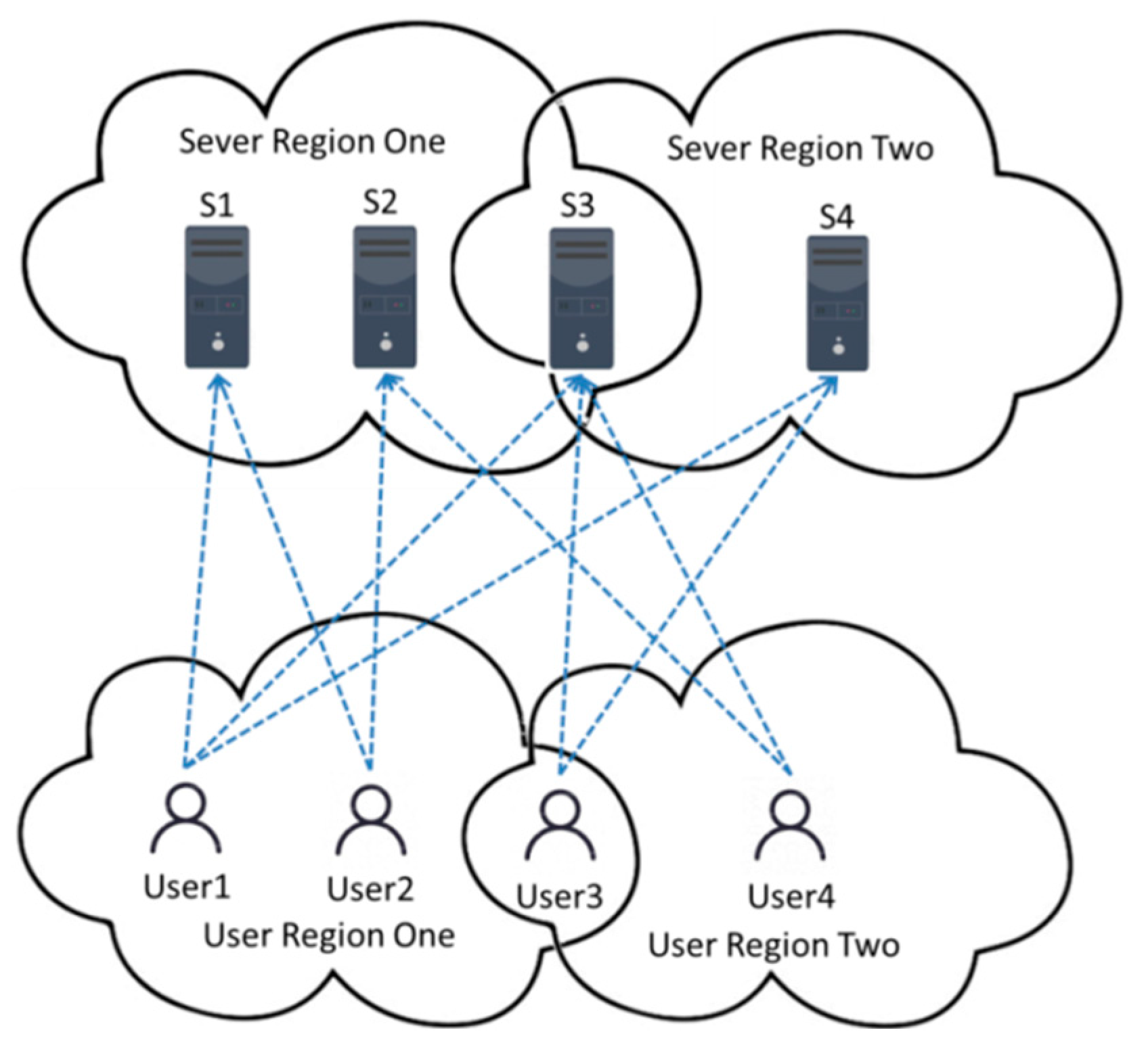
Figure 1 shows that User1, User2, and User3 are located in the same user region with similar location information, and the QoS values they invoke are also similar. Both S3 and S4 are located in service region two with a similar quality of service values. In practical scenarios, the environment and quality of the network are usually similar in terms of neighboring geographic locations, which plays an important role in the prediction of experience quality for different users. After the location projection, the number of records of users calling services and the number of users and services increase without introducing additional information. Thus, it is useful to take location information from users and services into account for game user perception evaluation prediction.
In real scenarios, the network is divided into idle time and busy time. These two concepts are relative. For example, busy time means that the network will be slower during the daytime when there are more people using or grabbing the network. The network speed will be faster during idle time. Different regions have different network usage habits, and the resulting idle time and busy time are also different. What we need to consider is that the basic network parameters (for players to enter the game during busy hours) are worse than those when they are idle, which will cause game users to perceive poorly. We need to understand the changes in user perception in different time periods, predict the user perception evaluation in different situations, and point out the direction for operators to choose optimization decisions to improve user perception. Our experiments are based on the Xinjiang University campus network. The time periods for teachers and students to access the Internet can be divided into four time periods, as shown in
Table 1.
We chose to test in the latter three time periods, to be more instructive, and divided into three time periods in chronological order: morning, midday, and evening. However, the busy hours in these three time periods are 13:00–15:00, 19:00–21:00, and 24:00–2:00, respectively. These three busy hours are the time periods when teachers and students take their meals and breaks. They are two overlapping areas in the three time periods, so using the idea of location projections, each busy time is divided into two, and two new time periods are obtained for each. Combining user and time information to obtain new features, we find two new pieces of game data after time projections. Our experiments are tested based on the Xinjiang University campus network, and the default user location information is similar, so we integrate the projections of both the location information and time information of the service into the new service matrix. The above two ideas expand our dataset without introducing additional information. However, this aggravates the challenge posed by data sparsity.
3.3. Similarity Calculation
Game user perception is a multidimensional nonlinear problem. In actual experiments, we found that under similar network conditions, different players or other conditions may lead to different final user perceptions. The features of each instance and its corresponding label are represented as an association, which is considered a correlation [
20,
21], similarity, or likelihood distribution [
22]. The relationship between each sample and its corresponding label can also be represented by the correlation. To address this issue, we introduce the fuzzy set theory, which uses a membership function to determine the similarity between data points and the centroid vector of each label.
In our work, the membership function is based on the similarity point of view, by the distance to the perfect sample-based similarity point of view [
23]. We adopt a multidimensional Gaussian function as the membership function [
24], which is widely used in many applications because of its simple form [
25]. The multidimensional membership function in our proposed method is defined as:
where
is the membership value and
. Here
is the dispersion of the radius,
is the inner product value of the feature interaction and
is the center vector of the corresponding label. The centroid vector
is calculated as follows:
where
,
is the
-th label corresponding to the instance
, and
is denoted as the element number of the set
. The membership function in Equation (2) is used to measure the similarity between the feature interaction and the centroid vector. If the sample value is close to the centroid vector, then its membership is higher. Conversely, its membership is lower the farther it is from the centroid vector.
3.4. LTFM Based on Fuzzy Set Theory
In this section, an LTFM model under the FM framework is proposed as a solution to the user game perception evaluation problem, as it has the advantage of capturing nonlinear feature interactions efficiently for sparse data. Unlike the standard FM model, LTFM takes the projection of location and time information into account. We construct an LTFM model that can effectively capture the projection information of location and time information as additional information without introducing additional information, and the similarity between feature interactions and labels obtained based on fuzzy set theory to improve the predictive strength of the model for user game perception valuation.
The structure of FM is shown in Equation (3). Inspired by this, our data will be encoded as
. Each element of
represents a user, and each element of
is a game service after time and location projections. The projection information of location and time information is integrated into the new service matrix, and the new data is represented as
, which is presented into the FM model’s pairwise feature interaction module, as shown below.
At this point, the LTFM can be expressed as
where
is the weight of the global bias, and
is the hidden vector of the
-th variable in
.
is the hidden vector of the
-th variable in
.
is the inner product of the hidden vectors of the user matrix and the service matrix. The inner product value can represent the pairwise interactions between the users and the services.
As introduced in the discussion in
Section 3.3, feature interactions that are less predictable are given lower weights since they contribute less to the game perception evaluation. The lack of ability to distinguish the predicted strength of pairwise feature interactions may lead to additional computational resources and suboptimal predictions. It means that embeddings of less important feature interactions are ignored. Thus, the similarity between pairwise interaction features and labels is captured in the output weights to reformat the pairwise part of FM as follows.
The calculation of is given in Equation (2), which considers the influence of the correlation between pairwise interaction features and labels on the predicted strength of the user’s game perception evaluation. The same can be applied to new feature interactions.
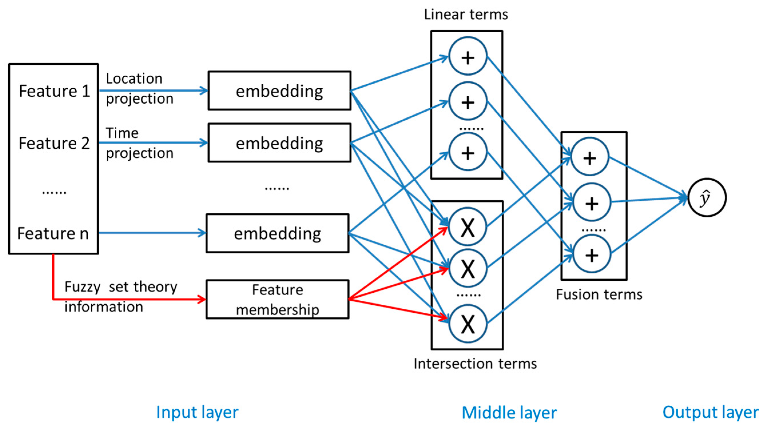
Combined with the above description, the final network architecture of our LTFM algorithm is shown in
Figure 2, which consists of three layers: the input layer, the middle layer, and the output layer.
The input layer: LTFM performs feature embedding based on the embedding matrix. Every feature is represented by dense vectors. It also can be seen as a fully connected layer, which implements array lookup. In the input layer, the key point is able to multiply the matrix fully. The inputs multiply with the weight matrix, which also takes the bias vector into consideration so that the spatial dimensionality and the projection of sparse to dense representations can be handled efficiently.
The middle layer: The model is inspired by the FM model. LTFM also needs to find how to represent the latent relationship in pairwise features which can be solved by the inner product. The set of pairwise feature interactions is represented as depending only on the embedding matrix. The middle layer has listed the potential vectors in interactions. The input layer has given feature embedding vectors. Each latent vector is the product of previous embedding vectors. Therefore, we use the idea of using neural networks to design and build into this layer to roughly express the FM model.
The output layer: We compress all feature interactions based on distinguishing their importance in the embedding space. Then, we project them onto the final perceptual prediction scores. The predicted similarity of a paired feature interaction is calculated based on Equation (2). In conclusion, the LTFM proposed in this paper can be expressed as follows.
In order to evaluate the parameters in Equation (8), the main method is to minimize the sum of losses on the observed dataset.
where
denotes the loss function and
denotes the regularization term on
, which is usually used to avoid overfitting. The overfitting problem cannot be ignored when optimizing machine learning models and FM models [
26]. In this study, our regularization term is
.
Neurons in paired interaction layers can easily cooperate with each other to adapt, which leads to overfitting. In this study, the LTFM model captures interactions that are predictive and useful. We control the regularization strength by the L2 regularization method and further prevent overfitting of the LTFM model by the dropout method on paired interaction layers [
27]. The dropout method prevents the complex cooperative adaptation of neurons to the training data. The main idea is to randomly drop out some neurons along the connections during the training process. The dropout module is applied for model training when the entire network architecture is used for prediction and is disabled for testing. Dropout has the additional side effect of using smaller neural networks for averaging, which may improve performance. Therefore, the dropout method is used in the middle-paired interaction layer of the LTFM model to deal with the overfitting problem.
The complexity analysis of our proposed LTFM model has the following two points. First, the parameters of the feature embedding matrix are . Thus, the entire spatial complexity of the LTFM model is , which means it is comparable to the standard FM model in terms of spatial complexity. The computational cost is . For model prediction, since the membership score is computed by fuzzy set theory techniques, the computational effort of the middle layer is reflected by the complexity of the inner product of the two vectors. The overall time complexity of the LTFM model is . In conclusion, our proposed LTFM algorithm can be trained in linear time. This complexity analysis shows that the LTFM model is very efficient.


