Abstract
The accurate identification of the shape of the blast furnace (BF) burden surface is a crucial factor in the fault diagnosis of the BF condition and guides the charge operation. Based on the BF 3D point cloud data of phased array radar, this paper proposes a 3D burden surface feature definition system. Based on expert experience, the feature parameters of the burden surface are extracted. The voxel feature was extracted based on improved BNVGG. The optimized PointCNN extracts the point cloud features. The features of the burden surface were defined from three perspectives: the surface shape, voxel, and point cloud. The research of the 2D burden line is extended to the 3D burden surface, and the assumption of the symmetry of the BF is eliminated. Finally, the accuracy of the burden surface classification under each feature was evaluated, and the effectiveness of each feature extraction algorithm was verified. The experimental results show that the shape feature defined based on expert experience affects the recognition of the burden surface. However, it is defined from the data perspective and cannot accurately identify a similar burden surface shape. Therefore, the voxel features and point cloud features of the burden surface were extracted, improving the identification accuracy.
1. Introduction
The BF ironmaking production process is the focus of the steel industry, and the development of steel intelligent manufacturing is an important direction for the transformation and upgrading of the industry [1]. The application of modern technologies such as industrial Internet and artificial intelligence to the steel manufacturing industry is of great significance to enhancing the comprehensive competitiveness of the steel industry [2].
The traditional method uses diverse sensors to detect the burden surface and obtain multi-source data. The burden surface detection instruments include the height and temperature sensors [3]. Height sensors use multiple radars or mechanical probes to measure different points on the burden surface and then reconstruct the non-sampling points according to the mechanism model method or the fitting method [4]. The temperature sensors, using cross-temperature measurement methods, obtain the temperature distribution map by interpolation and reconstruct the burden surface [5].
The burden surface can reflect the production status and thus guide the upper adjustment of the BF. In actual production, the accuracy and adaptability of the burden surface model are the key factors to ensuring the normal operation of the smelting process [6]. The complex environment inside the BF makes it difficult to measure the data, so the 2D burden line is often used to describe the 3D burden surface. The 2D burden line data are from the height value of the sparse discrete data points, and the radial burden line is obtained by interpolating or fitting the data [7]. Liu described the shape of the burden surface in two straight lines [8]. Guan et al. established the distribution model of the burden surface by using two straight lines and two curves [9]. Zhu et al. used two straight lines and one curve to describe the shape of the burden surface [10]. Matsuzaki described the charge distribution using a single functional equation [11]. In the asymmetric state, a single fitted burden line cannot represent the entire burden surface, and the burden line’s fitting model has a large error, which leads to losing a lot of information about the burden surface.
The feature parameters of the burden surface can accurately reflect the real production status. Li et al. pointed out that the two key factors of the BF charge control are the width of the surface platform and the depth of the funnel [12]. Based on expert experience, Zhang et al. proposed a method for defining and extracting six features that can characterize the shape of the burden surface [13]. However, the above research also extracted and defined the features of the 2D burden line. How to define the 3D burden surface feature is the focus of this manuscript.
Based on the phased array radar point cloud data, this manuscript proposes a method for defining the characteristics of the BF 3D burden surface. Based on expert experience, 18 sets of burden surface features were defined and extracted. To solve the problem that similar burden surfaces cannot be accurately classified from the data perspective, we use the BNVGG network to extract the 2D voxel features [14] and use PointCNN to extract the 3D point cloud features [15]. Through these three sets of features, the correct identification of the burden surface is realized, which lays the foundation for charge operation, a historical burden surface database, fault diagnosis, etc.
This manuscript is divided into five sections. The second section introduces a 3D burden surface feature definition method based on expert experience. The third section is a 2D voxel feature extraction method based on BNVGG and a 3D point cloud feature extraction method based on PointCNN. The fourth section is about the simulation results. The fifth section has the conclusion, which summarizes the main content of the manuscript and future work.
2. 3D Burden Surface Feature Parameter Definition
The 3D burden surface can truly reflect the condition information of the BF, and the feature parameters can accurately reflect the real production situation. The new phased array radar measurement device successfully solves the problem of measuring the burden surface by accurately detecting the feeding situation of the BF in all directions, increasing the detection point to more than 2000 points. By analyzing the point cloud data detected by phased array radar, the mathematical geometric characteristics of the burden surface are summarized, and the feature definition strategy is designed based on expert experience. The extracted features can realistically reflect the 3D surface shape and help analyze the furnace condition.
2.1. Phased Array Radar
BF ironmaking is a typical “black box” system with nonlinearity, time lag, and noise. Despite the substantial number of inspection devices installed, measurement of the 3D burden surface is still difficult to achieve. If this point can be broken, it will improve the level of charge control and help the burden surface research.
The traditional detection method is limited by data points, which cannot fully reflect the actual situation of the burden surface. Industrial phased array radar detection technology can scan the entire burden surface of the BF, which has the characteristics of flexible beam direction, strong adaptability to complex environments, and good anti-interference performance [16]. Kundu C successfully solved the problem of direct measurement of the burden surface by developing a new phased array radar measuring device and increasing the detection point to more than 2000 points [17]. The high-resolution image of the burden surface acquired by the phased array radar is shown in Figure 1. From bottom to top, each burden surface corresponds to a charging process.
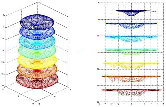
Figure 1.
A high-resolution image of the burden surface.
From the figure, the height of the burden surface and the position of the furnace wall can be found. The burden surface fluctuates in various places, and the furnace wall can also have an impact. Through the multi-point detection technology of industrial phased array radar, the entire burden surface’s height information can be obtained. Compared with other radar detection methods, phased array radar can obtain more detection data, and the 3D burden surface contains more shape information, providing a data basis for subsequent research.
2.2. 3D Burden Surface Feature Parameter Definition
Zhang proposed three 3D burden surface definition methods: linear definition, ring definition, and sector definition. However, this definition method still follows the defined strategy of the burden line, which has certain limitations. The 3D burden surface is an irregular spatial surface. At present, no researchers have systematically proposed a clear method for defining this.
Based on the phased array radar point cloud data, a 3D burden surface feature definition method is proposed. The extracted feature parameters can reflect the shape of the burden surface well, which is helpful for the operator to understand the internal charge operation of the BF.
Combined with the experience of on-site experts, the definition of burden surface features should be universal. Eighteen surface feature parameters were determined, as shown in Figure 2. In the figure, the spatial 3D burden surface is divided into three areas: the central coke area , the funnel area , and the platform area . The spatial 3D burden surface shape is fitted by the three-segment ruled surface method. Once the equations of the highest point and the three characteristic curves , , and are determined, the spatial burden surface equation can be determined [18].
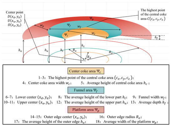
Figure 2.
3D burden surface feature parameters.
Using the parametric equation of the space curve to correlate the curve equations of two dimensions, the equations of the characteristic curves , , and are obtained:
The parametric equations of three region surfaces , , and are as follows:
The complete burden surface equation obtained by fitting is . The results of the area surface fitting are shown in Figure 3.
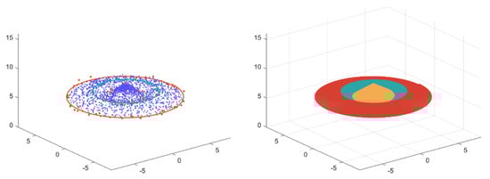
Figure 3.
Characteristic curve definition (left) and area surface fitting (right).
After the burden surface fitting process is completed, 18 feature parameters are extracted. The highest point in the central focal area is directly obtained from the point cloud data. The center points , , and and the radii , , and are obtained by the least square method, and the calculation formulas of the remaining eight features are as follows.
The center focus area width is :
The average height of the central coke area is :
The average height of the lower part of the funnel is :
The average height of the upper part of the funnel is :
The funnel width is :
The average depth of the funnel is :
The average width of the platform is :
The average height of the outer edge of the burden surface is :
This method defines 18 3D burden surface features, which will be used as the main index parameters of subsequent research.
Based on the phased array radar data, a 3D burden surface feature definition method is proposed in this section. According to the burden surface structure, it is divided into three areas: the central coke area, the funnel area, and the platform area. Fitting each area with the three-segment method is performed to extract the feature parameters. The extracted feature parameters can reflect the surface shape, providing visual and accurate support for the operator’s cloth operation. Depending on the feature parameters of the different regions, the abnormal area of the failed burden surface can be quickly determined. This is helpful for surface recognition and troubleshooting.
3. 3D Burden Surface Feature Extraction
The feature definition method based on expert experience is for studying the geometry of the 3D burden surface. The surface shapes are defined by transforming them into points, lines, and surfaces. This method is suitable for distinguishing faulty surfaces that differ from normal conditions, but there are similarities in the surface types under certain furnace conditions, and these are difficult to accurately classify from a data perspective.
To solve the above problems, the burden surface depth feature extraction schemes are designed. First, the classical VGG network structure is optimized, and the BNVGG network is designed to extract the voxel features of the burden surface. Second, the optimizer of PointCNN is tweaked, and a learning rate decay strategy is added. The improved PointCNN network is used to extract the point cloud features. The machine learning method is used to mine the depth features and achieve the purpose of accurate identification of the burden surface.
3.1. Voxel Feature Extraction by BNVGG
The traditional convolutional neural network (CNN) is very mature in 2D images, but due to the out-of-order nature of the point cloud data, it is difficult for CNNs to be directly applied to point clouds. We transform the 3D models into Euclidean spaces such as image regions, voxel regions, or primitive regions to accommodate traditional deep learning methods.
The term voxel is a combination of pixel, volume, and element, being equivalent to pixels in 3D space. Through standard meshing, the coordinates of the burden surfaces are aligned, and each corresponds to a different z. The 3D burden surface data are converted into a 2D array, and their voxel features are extracted. The results of this meshing are shown in Figure 4.
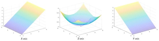
Figure 4.
The burden surface meshing.
VGGNet is a deep convolutional network structure proposed by the Visual Geometry Group (VGG) of the University of Oxford [19]. In VGG, three 3 × 3 convolution kernels are used instead of 7 × 7 convolution kernels, and two 3 × 3 convolution kernels are used instead of 5 × 5 convolution kernels. The main purpose of this is to increase the depth of the network, reduce the parameters, and improve the effectiveness of the neural network to a certain extent under the condition of ensuring that it has the same sensing field. The network structure of VGGNet is shown in Figure 5.
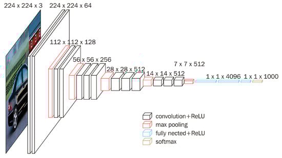
Figure 5.
The network structure of VGGNet.
Following the concept of the convolution kernel in VGGNet, the network structure is optimized, and a BN layer is added after each convolutional layer [20]. We call the optimized network structure BNVGG. The BN layer normalizes the features of the output of the convolutional layer; that is, it converts the input data into a normal distribution with zero as the mean and one as the variance.
where , w is the weight of the layer, and u is the output of the previous layer. This operation increases the derivative value of the activation function and makes convergence occur faster:
where the and parameters can be learned through backpropagation, through which the data are expanded and translated to restore the distribution of some features.
The optimized network structure is shown in Figure 6, which includes nine convolutional layers, three maximum pooling layers, and four fully connected layers. Among them, the activation functions of the convolutional layer and the fully connected layer are both ReLU functions.
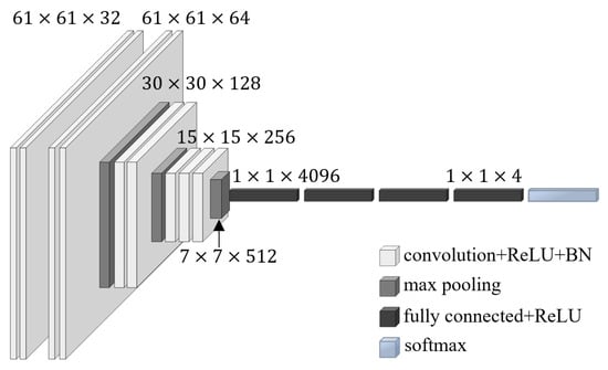
Figure 6.
The network structure of improved BNVGG.
We set the neural network parameters of BNVGG. The batch size was set to 30, the momentum was , and the learning rate was set to . Training was regularized by weight decay (L2 penalty multiplier set to ), and the first two fully connected layers took dropout regularization (dropout ratio set to ). Then, 128 features were extracted from the third fully connected layer (FC-128) and transformed into dimensions to obtain a voxel feature matrix of the 3D burden surface, which was saved and used for subsequent research.
3.2. Point Cloud Feature Extraction
Most of the feature extraction methods for the burden surface are extracted by dimensionality reduction or expert experience. These extraction methods generally do not have high utilization and introduce quantization artifacts that may mask the natural invariances of the data. To solve the above problems, PointNet and PointCNN, which specialize in processing point cloud data, were used to extract the features and compare the results with other feature extraction methods.
3.2.1. PointNet
PointNet is a network model specifically for training point cloud data proposed by R. Q. Charles in 2017 [21]. The network structure is shown in Figure 7.
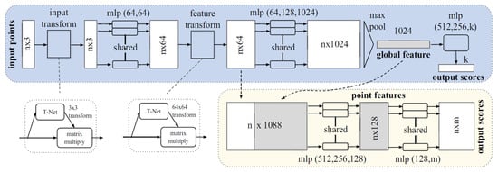
Figure 7.
The network structure of PointNet.
The PointNet network takes n points in a set of point clouds as input, each containing three dimensions . Then, the input data are spatially transformed. The feature transformation is realized through the convolutional layer. Then, the feature space is spatially transformed, and the feature is reduced in the maximum pooling layer to obtain the compressed global feature. Finally, the high-dimensional features are fused by the fully connected layer, and the score of the point in each class of K is the output. It is an extended network of classification networks that fuses the local features of each point and outputs the score of each point belonging to each part.
The PointNet network has three key modules:
- 1.
- It uses the maximum pooling layer as a symmetric function that aggregates information from all points. The high-dimensional features extracted from the point cloud converge through a symmetry function and finally approach the function defined on the point set:Here, h is simulated by a multilayer perceptron (MLP) and combined with the maximum pooling function to simulate g. With the set of h, the network can learn f to capture different properties of the point cloud data.
- 2.
- The structure combines the local and global features. After calculating the global features of the point cloud data, the global features and the local features of each point are connected as a new feature matrix, and then the new features of each point are extracted from the new feature matrix so that the local and global information is considered for each point.
- 3.
- Two federated alignment networks rotate and align each point and feature in the point cloud data. PointNet uses T-net to learn the structure of point cloud data and obtain a spatial transformation matrix. This method can be extended to feature space alignment. We add another T-net network after the convolutional layer to learn the feature structure information of this layer and perform spatial transformation processing on the current high-dimensional features. However, the dimensionality of the features is much higher than that of the point cloud data, which leads to increased computational complexity, making it hard to converge. The orthogonal transformation matrix does not lose information, so PointNet adds the orthogonalization function of the transformation matrix to the final loss function:Here, A is the spatial transformation matrix learned by T-net, which has the effect of aligning features.
We build PointNet and adjust the network hyperparameter separately to realize the feature extraction of the burden surface. The network structure is shown in Figure 8.
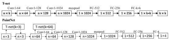
Figure 8.
The network structure of T-net and PointNet.
In the first T-net, , corresponding to the coordinate values, realizes the rotationally symmetric transformation of the point cloud data. The second T-net () outputs a 64-dimension spatial transformation matrix. This T-net is the point cloud data after a convolution transformation, and the characteristics of the obtained points are data-aligned. The final output is a matrix representing four types of the burden surface. This method implements classification through the last fully connected layer (FC-4). The output results are also used for the calculation of loss values and the adjustment of network parameters. A total of 256 features were extracted from the fully connected layer (FC-256), and a point cloud feature matrix was obtained, which was used for subsequent research.
In the training of the network model, the stochastic gradient descent (SGD) optimizer is replaced by the Adam optimizer. The Adam optimizer can automatically fine-tune the learning rate for each different network parameter during the training process to achieve a better convergence effect. An attenuation strategy is designed for the learning rate so that it can automatically decrease with the increase in the number of training iterations, thereby reducing the possibility of mutation of the results and reducing the frequency of glitches.
3.2.2. PointCNN
The PointCNN is a method for processing point cloud data proposed by Li Y in 2018. PointCNN defines a transformation matrix with dimensions . The function of the transformation matrix is to regularly sort and weight the out-of-order point cloud data to obtain a new set of data. This new set of data has a certain order, and the data elements have adjacent position information, and then ordinary convolution operations can be used to achieve feature extraction. Based on the above ideas, PointCNN proposes the -Conv operation to replace the traditional convolutional operation. The algorithm is expressed as follows:
Here, K is a convolution kernel with dimensions , p represents the point cloud data to be convolved or the feature set extracted from the previous layer, P is the neighbor point set, and F is the feature set of the neighbor points. For -Conv, the operation process is as follows.
Algorithm 1 calculates the adjacent point set P of each point in p before the -Conv operation. In this step, the KNN algorithm or random sampling can be used to extract the neighbor point set P and then follow the following process:
- 1.
- Subtract the coordinates of point p from the coordinates of each neighbor point and obtained the relative coordinates of the point.
- 2.
- The location information of neighboring points is converted into feature vectors through an network.
- 3.
- Splice the transformed features with their own features to obtain new features.
- 4.
- Calculate the -matrix through the network, corresponding to the current input.
- 5.
- Use the -matrix to process the feature matrix of a specific order.
- 6.
- Perform convolution operations to obtain the future of the p point set.
| Algorithm 1-Conv operator. | |
| Input: | |
| Output: | ▹ Features “projected”, or “aggregated”, into representative point p |
| ▹ Move to local coordinate system of p |
| ▹ Individually lift each point into dimensional space |
| ▹ Concatenate , and is a matrix |
| ▹ Learn the -transformation matrix |
| ▹ Weight and permute with the learned |
| ▹ Finally, typical convolution between and |
The algorithm flow can be expressed as follows:
According to the core ideas elaborated upon by Li Y et al., PointCNN is built based on -Conv. Each -Conv has four basic properties of K, D, P, and C. K represents the number of neighboring points, D represents the expansion coefficient, P represents the number of points, and C represents the number of channels (characteristic dimension) of the output. The three inputs are the point set p that needs to be extracted from the features, the representative point set q, and the feature vector set F. The size of the representative point set q needs to be consistent with the point set p, and q is a subset of p. The flow of the -Conv operation is as follows:
- 1.
- Neighbor sampling: The KNN algorithm is used to find nearest neighbors for each representative point in q, and the interval D sampling is decimated to obtain the nearest neighbor point set matrix.
- 2.
- Decentralization: Subtract the corresponding representative point coordinates from each set of neighbor coordinates to obtain the relative coordinate matrix of the near neighbor points.
- 3.
- Feature splicing: The relative coordinate matrix boosts the dimensions through two fully connected layers and is spliced with the input feature vector set F to obtain a new set of features.
- 4.
- Calculation transformation -matrix: The relative coordinate obtained by step 2 is processed, and the coordinate-related features are extracted to obtain a set of a transformation -matrix.
- 5.
- Conduct transformation -matrix: The features extracted in step 3 are combined with the transformation -matrix to obtain a new feature matrix.
- 6.
- Feature transformation: New features are extracted and elevated to the C dimension.
The process in step 4 is shown in Figure 9.
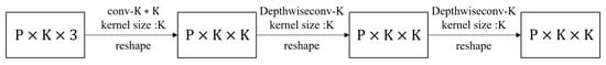
Figure 9.
Transformation -matrix.
The calculation of the transformation -matrix first performs a conventional convolution operation through K × K convolution kernels, which promotes the feature dimension to the K dimension. Then, two depth-wise convolutions are conducted while keeping the feature dimension unchanged. The use of a deep convolutional layer here to increase the influence of each channel individually, on the one hand, is conducive to feature extraction, and on the other hand, it also reduces the parameters in the calculation.
For a sampling of the nearest neighbor points in step 1, the expansion rate D is introduced into the -Conv. It acts as a perforated convolution to improve the information contained in the extracted features.
We built a PointCNN based on -Conv, and the structure is shown in Figure 10.
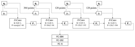
Figure 10.
The PointCNN based on -Conv.
In the first layer of -Conv, the point set p is processed as representative points, and the feature of each point is extracted, where . The subsequent -Conv layer takes the previous representative point as the point set of the feature processing; that is, , and it randomly extracts a certain number of points as the representative point of this -Conv. The network structure is such that with the increase in the number of layers, the number of extracted representative points P decreases, and the feature dimension C increases, which is similar to a CNN, increasing the depth of the feature channels and reducing the number of input points. The number of neighboring points K increases correspondingly with the expansion rate D, and the point set p used to sample the near neighbors is sparser, which will make each feature fuse more point cloud information. This means that the previous layer integrates the local information of the point cloud and gradually increases the scale of integration until the deeper layer has more macroscopic information for data extraction and reflects the global structure information of all of the point cloud data.
In the PointCNN network structure, the last three layers are fully connected layers that aim to fuse and classify the features of the extracted data. The last fully connected layer also plays a simple classification role, realizing four classifications of compressed features. In the penultimate fully connected layer, this experiment also adds a dropout layer, which sets the probability of discarding at so that each feature value output by FC-192 discards of each training time to prevent data overfitting. The Adam optimizer is still selected to optimize the gradient of the output results of the network model, which increases the adaptability of the learning rate. As in PointNet, the learning rate decay strategy is set to reduce the learning rate to every thousand iterations.
This section mainly introduces the frameworks and principles of BNVGG, PointNet, and PointCNN. The network model was built and optimized to extract and classify the feature of the 3D burden surface.
4. Results
From Figure 11, the burden surface data were acquired using phased array radar and divided by expert experience into (a) normal, (b) center is too high, (c) funnel is too large, and (d) coke is too much. These four types of surfaces each had 1000 sets of data. Through the classification experiment, the accuracy of the burden surface recognition under each feature was verified. The training and test sets were at a ratio of 7:3.
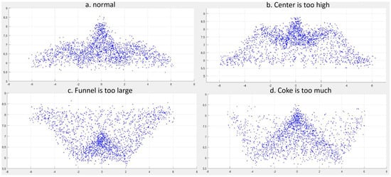
Figure 11.
Four types of burden surfaces.
The four sets of feature parameters of the burden surface, based on expert experience, are shown in Table 1. These feature parameters can reflect differences among the burden surface. For example, the parameter of the (d) group was significantly larger than that for the other surfaces, indicating that there was too much central coking. Group (c) had an oversized parameter, indicating an oversized funnel area, and so on.

Table 1.
Part of the feature parameters.
4.1. Feature Parameter Results
Based on expert experience, 18 feature parameters of 4 types of surfaces were calculated. We converted the feature parameters into a 1 × 18 feature matrix and input that into the GWOKEM classification algorithm. The ratio of the training set to the test set was 7:3; that is, 2800 sets were training sets, and 1200 sets were test sets. The performance of this algorithm has been experimented with in previous articles and will not be repeated in this article. The classification results are shown in Figure 12.
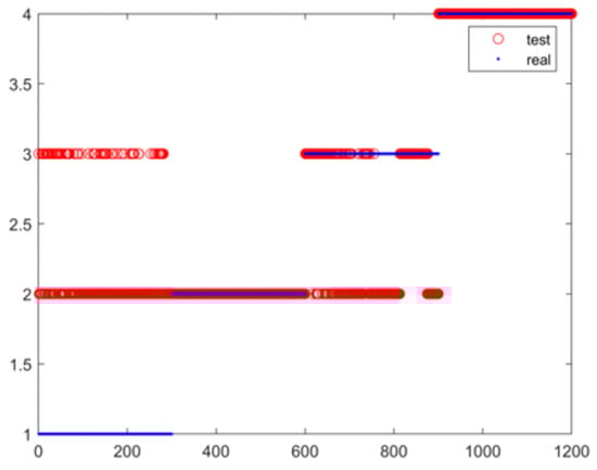
Figure 12.
Classification results of the feature parameters.
The feature parameters contain shape information of the burden surface, such as the depth, width, and radius. Based on this underlying mathematical shape information, specious surface shapes that are difficult to recognize in neural networks can be excluded. The center coke area, funnel area, and platform area contain their own feature parameters to facilitate a quick search of the fault area. In contrast to the depth features (voxel features and point cloud features), each feature parameter has mathematical significance and is solvable.
The ordinate represents the surface category, and the abscissa is the test set designator. The accuracy of the test set was about . From the classification results of the feature parameters, the recognition accuracy of (a) and (c) was low. This was due to the similarities between the two sets of surfaces, which made accurate classification difficult from a data perspective. Therefore, it was necessary to extract the voxel features and the point cloud features.
4.2. BNVGG Results
The network structure of traditional VGG was optimized, the number of network layers was simplified, the training time was reduced, and the BN layer was added to improve the network convergence speed and reduce the number of iterations. The training results of BNVGG were compared with VGG16, ResNet, and AlexNet to verify the performance of the network structure.
From Table 2, the accuracy of BNVGG for the burden surface recognition was better than that of other neural networks for the same number of iterations, and BNVGG can converge faster than VGG16. It was verified that the BNVGG network structure had good training and classification effects on the current experimental subjects.
Table 2.
Algorithm performance comparison.
4.3. PointNet Results
The point cloud data of the burden surface were put into the model and trained. After the hyperparameters were adjusted, the learning rate had a more significant impact on the experimental results. If the learning rate was too large, the network would oscillate significantly during the convergence process, and it would not be easy to converge to a stable state. Additionally, the optimal solution may have been skipped, resulting in overfitting. If the learning rate was too small, the convergence would be slow. It needed to iterate multiple times to reach the optimal interval, which greatly wasted the amount of calculation and time and would also lead to convergence in the suboptimal solution. After many trials, the initial learning rate was set to . The training process is shown in Figure 13.
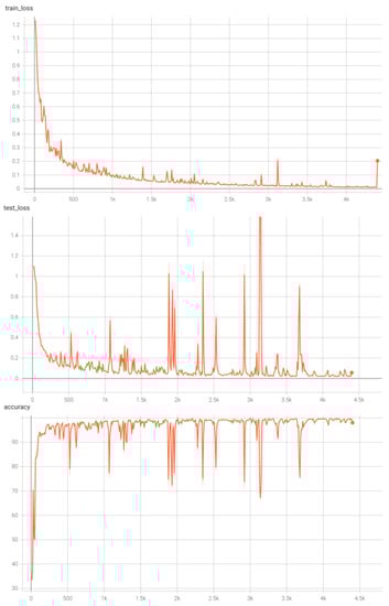
Figure 13.
PointNet training curve (no learning rate decay).
From top to bottom, the train loss curve, test loss curve, and test accuracy curve are shown. The training results tended to converge, and the loss value of the training set decreased steadily with the increase in the number of iterations. The accuracy rate of the test set gradually increased, which shows that the network did have a classification effect. However, it can be seen from the figure that the final accuracy rate curve still had oscillations, and the results of the training model were unstable. During the training process, there were many glitches on the curve, and the accuracy rate at the lowest point was only about . Therefore, a learning rate-decreasing strategy was added to the training process. After every 400 steps of iterative training, the learning rate was reduced by . Based on this strategy, the initial learning rate was adjusted to to speed up the convergence, reduce the amount of computation, and shorten the computation time. The learning rate curve during training is shown in Figure 14.
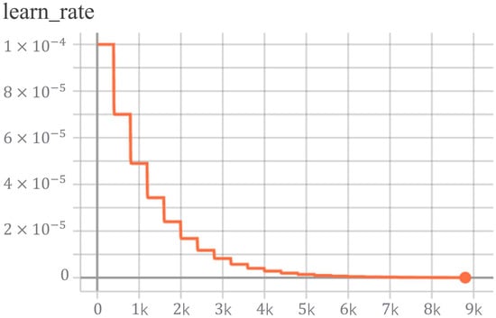
Figure 14.
Learning rate curve.
The network training results based on the learning rate strategy are shown in Figure 15.
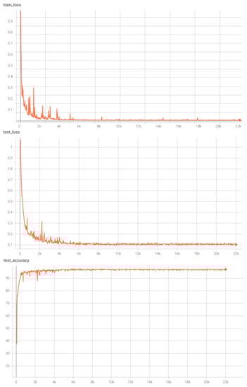
Figure 15.
PointNet training curve (learning rate decay).
At the beginning of training, due to the large learning rate, the loss curve and accuracy curve fluctuated greatly, resulting in unstable training results. However, as the learning rate decreased, the curve gradually stabilized and approached convergence. Compared with the curve before adding the learning rate decay strategy, the curve in the later stage of training was more stable, and almost no glitches were generated. It can be intuitively reflected that the training tended to converge, and the accuracy curve was stable. The final test accuracy rate reached about , which verified the performance of the network.
4.4. PointCNN Results
We put the point cloud data into the PointCNN for training after setting the parameters. The training results are shown in Figure 16.
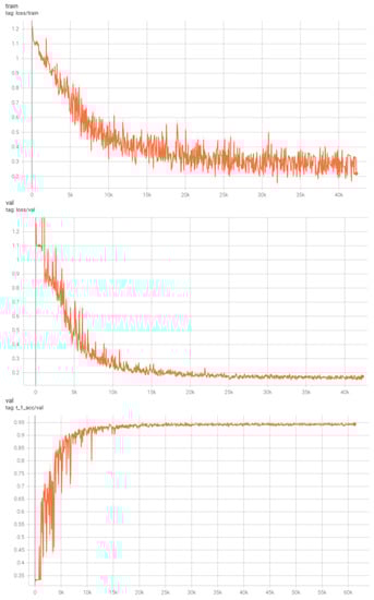
Figure 16.
PointCNN training curve (learning rate decay).
Compared with the training process of PointNet, the PointCNN had more twists and turns, and the amplitude during training was larger. From the accuracy curve of the test set, the accuracy of model classification was finally maintained at about , which was still far behind PointNet’s . The experimental results show that the PointNet network was better than the PointCNN network. PointNet has better performance in the feature extraction and classification of the burden surface.
The network structure of PointNet is relatively simple, and the number of network layers is relatively shallow. The feature extraction part is only composed of a normal training network plus two T-net symmetrical transformation networks. The network structure of PointCNN is relatively complex, consisting of four -Conv, and in each -Conv unit, the data need to go through at least three convolutional layers, which is better in terms of network depth, and the PointCNN network model uses fewer parameters during training. The situation of PointCNN is better than that of PointNet mentioned in the literature, but that was not reflected in this experiment. I personally think that this was caused by too little burden surface data and PointCNN overfitting, because for a deeper network, theoretically, the fitting effect is better, but the difficulty of network training will also increase. Due to the small data set, the burden surface feature information in the training samples was not perfect, and it was more difficult to extract features during deep learning, and thus overfitting occurred. It can be seen from the network structure of PointNet that after the maximum pooling layer, the extracted features were global features, and its classification model used the classification of global features and did not process the local features. However, PointCNN only uses convolution for feature extraction, which makes it easier to retain the local information of the processed data. Therefore, the PointNet network model is more dominant in the problem of global feature processing of the burden surface data.
Table 3 shows the accuracy of the burden surface recognition under the three features.
Table 3.
The accuracy of recognition under each features.
5. Discussion
A 3D burden surface feature definition system was proposed in this manuscript. We divided the burden surface into the central coke area, funnel area, and platform area. Based on expert experience, the feature parameters for each region were defined and extracted. The feature parameters contain the shape information of the burden surface. Based on this underlying mathematical shape information, specious surface shapes that are difficult to recognize in neural networks can be excluded. The depth features (voxel features and point cloud features) were extracted based on improved BNVGG and PointCNN. Deep learning of the burden surface can improve the accuracy of recognition. The 3D burden surface feature definition system is perfected through different angles, which lays the foundation for the subsequent matching of surface types, fault diagnosis, and the establishment of the surface history database. Experiments have verified the accuracy of burden surface recognition under each feature. The following conclusions were obtained through the analysis of the experimental results of Section 4:
- 1.
- The 18 feature parameters based on expert experience can accurately classify some burden surfaces with obvious differences, but they are difficult to classify on similar shapes. The accuracy of the test set was about 65.37%. It defined the shape of the burden surface from the perspective of the data and had a certain reference value.
- 2.
- We extracted the voxel features of the burden surfaces by the optimized BNVGG network. The accuracy of the burden surface recognition was increased (95.67%), and the time of network training was reduced (238 s). The comparative experiment verified the effectiveness of the network structure, which had good identification and classification effects on the burden surface data.
- 3.
- The two neural network models of PointNet (96.5%) and PointCNN (94.4%) can obtain better results when processing point cloud data. PointNet implements the extraction and classification of the global features, while PointCNN realizes the extraction of the global and local features of the burden surface data. However, due to the particularity of the burden surface data, the local feature part of PointCNN has no effect. In the extraction of global features, PointNet’s performance is better, and it is more suitable for the feature extraction and classification of the burden surface.
According to the experimental results, in subsequent research, some objectives are the following:
- Increase the scale and category of the data before training. By increasing data complexity, the advantages and disadvantages of deep neural networks can be reflected.
- Due to the difficulty of obtaining the original data, the generative confrontation network can be used to learn the original data features and generate more authentic simulation data.
- The neural network is trained through various feature parameters, determining by trial and error the optimal topology of the neural network, the number of hidden layer nodes, and the neural network layer transfer function. This method provides a new idea for network training [24,25].
- For the three types of features extracted in this manuscript, the feature fusion operation is performed through the method of attention mechanism. The fusion features could be used to test the effect of burden surface recognition.
- Through the effective fusion of the features of burden surfaces and the parameters of furnaces, the matching and fault diagnosis of new burden surface data could be achieved.
The feature parameters and the voxel and point cloud features are fused based on the attention mechanism, and a feature matrix is established. The original point cloud data can be replaced with this feature matrix. Then, by means of the double clustering algorithm, the feature parameters of the BF state are fused with the matrix of the burden surface features to produce a new feature matrix. This feature matrix is used to troubleshoot the BF and match the burden surface.
Author Contributions
Conceptualization, S.S., Z.Y. and S.Z.; methodology, S.S.; software, S.S. and Z.Y.; validation, S.S. and Z.Y.; formal analysis, S.S.; investigation, S.S.; data curation, S.S.; writing—original draft preparation, S.S.; writing—review and editing, S.Z.; visualization, S.S.; supervision, S.Z. and W.X.; project administration, S.Z. All authors have read and agreed to the published version of the manuscript.
Funding
This work was supported by the National Natural Science Foundation of China under Grant No. 62173032 and Grant No. 62003038 and the Natural Science Foundation of Beijing Municipality under Grant No. J210005.
Institutional Review Board Statement
Not applicable.
Informed Consent Statement
Not applicable.
Data Availability Statement
Not applicable.
Conflicts of Interest
The authors declare no conflict of interest.
References
- Zhang, H.; Sun, S.; Zhang, S. Precise Burden Charging Operation During Iron-Making Process in Blast Furnace. IEEE Access 2021, 9, 45655–45667. [Google Scholar] [CrossRef]
- Zhao, J.; Zuo, H.; Wang, Y.; Wang, J.; Xue, Q. Review of green and low-carbon ironmaking technology. Ironmak. Steelmak. 2020, 47, 296–306. [Google Scholar] [CrossRef]
- Zankl, D.; Schuster, S.; Feger, R.; Stelzer, A.; Scheiblhofer, S.; Schmid, C.M.; Ossberger, G.; Stegfellner, L.; Lengauer, G.; Feilmayr, C.; et al. BLASTDAR—A large radar sensor array system for blast furnace burden surface imaging. IEEE Sens. J. 2015, 15, 5893–5909. [Google Scholar] [CrossRef]
- Xu, T.; Chen, Z.; Jiang, Z.; Huang, J.; Gui, W. A real-time 3D measurement system for the blast furnace burden surface using high-temperature industrial endoscope. Sensors 2020, 20, 869. [Google Scholar] [CrossRef] [PubMed]
- An, J.Q.; Peng, K.; Cao, W.H.; Wu, M. Modeling of high temperature gas flow 3D distribution in BF throat based on the computational fluid dynamics. J. Adv. Comput. Intell. Intell. Inform. 2015, 19, 269–276. [Google Scholar] [CrossRef]
- Li, Y.; Zhang, S.; Zhang, J.; Yin, Y.; Xiao, W.; Zhang, Z. Data-driven multiobjective optimization for burden surface in blast furnace with feedback compensation. IEEE Trans. Ind. Inform. 2019, 16, 2233–2244. [Google Scholar] [CrossRef]
- Shi, Q.; Wu, J.; Ni, Z.; Lv, X.; Ye, F.; Hou, Q.; Chen, X. A blast furnace burden surface deeplearning detection system based on radar spectrum restructured by entropy weight. IEEE Sens. J. 2020, 21, 7928–7939. [Google Scholar] [CrossRef]
- Liu, Y.C. The Law of Blast Furnace. Metall. Ind. Press 2006, 25, 54–57. [Google Scholar]
- Guan, X.; Yin, Y. Multi-point radar detection method to reconstruct the shape of blast furnace material line. Autom. Instrum. 2015, 36, 19–21. [Google Scholar]
- Zhu, Q.; Lü, C.L.; Yin, Y.X.; Chen, X.Z. Burden distribution calculation of bell-less top of blast furnace based on multi-radar data. J. Iron Steel Res. Int. 2013, 20, 33–37. [Google Scholar] [CrossRef]
- Matsuzaki, S. Estimation of stack profile of burden at peripheral zone of blast furnace top. ISIJ Int. 2003, 43, 620–629. [Google Scholar] [CrossRef]
- Li, C.; An, M.; Gao, Z. Research and Practice of Burden Distribution in BF. Iron Steel Beijing 2006, 41, 6. [Google Scholar]
- Zhang, H.; Zhang, S.; Yin, Y.; Zhang, X. Blast furnace material surface feature extraction and cluster analysis. Control. Theory Appl. 2017, 34, 938–946. [Google Scholar]
- Ding, X.; Zhang, X.; Ma, N.; Han, J.; Ding, G.; Sun, J. Repvgg: Making vgg-style convnets great again. In Proceedings of the IEEE/CVF Conference on Computer Vision and Pattern Recognition, Nashville, TN, USA, 20–25 June 2021; pp. 13733–13742. [Google Scholar]
- Li, Y.; Bu, R.; Sun, M.; Wu, W.; Di, X.; Chen, B. Pointcnn: Convolution on x-transformed points. In Proceedings of the Advances in Neural Information Processing Systems, Montréal, QC, Canada, 3–8 December 2018; p. 31. [Google Scholar]
- Wei, J.D.; Chen, X.Z. Blast furnace gas flow strength prediction using FMCW radar. Trans. Iron Steel Inst. Jpn. 2015, 55, 600–604. [Google Scholar] [CrossRef][Green Version]
- Kundu, C.; Patra, D.; Patra, P.; Tudu, B. Burden Profile Measurement System for Blast Furnaces Using Phased Array Radar. Int. J. Recent Eng. Res. Dev. 2021, 6, 24–47. [Google Scholar]
- Sun, S.S.; Yu, Z.J.; Zhang, S.; Xiao, W.D.; Yang, Y.L. Reconstruction and classification of 3D burden surfaces based on two model drived data fusion. Expert Syst. Appl. 2022, 119406. [Google Scholar] [CrossRef]
- Simonyan, K.; Zisserman, A. Very deep convolutional networks for large-scale image recognition. arXiv 2014, arXiv:1409.1556. [Google Scholar]
- Santurkar, S.; Tsipras, D.; Ilyas, A.; Madry, A. How does batch normalization help optimization? In Proceedings of the Advances in Neural Information Processing Systems, Montréal, QC, Canada, 3–8 December 2018; p. 31. [Google Scholar]
- Charles, R.Q.; Su, H.; Kaichun, M.; Guibas, L.J. Pointnet: Deep learning on point sets for 3d classification and segmentation. In Proceedings of the IEEE Conference on Computer Vision and Pattern Recognition, Honolulu, HI, USA, 21–26 July 2017; pp. 652–660. [Google Scholar]
- He, K.; Zhang, X.; Ren, S.; Sun, J. Deep residual learning for image recognition. In Proceedings of the IEEE Conference on Computer Vision and Pattern Recognition, Las Vegas, NV, USA, 27–30 June 2016; pp. 770–778. [Google Scholar]
- Krizhevsky, A.; Sutskever, I.; Hinton, G.E. Imagenet classification with deep convolutional neural networks. Commun. ACM 2017, 60, 84–90. [Google Scholar] [CrossRef]
- Esfe, M.H.; Eftekhari, S.A.; Hekmatifar, M.; Toghraie, D. A well-trained artificial neural network for predicting the rheological behavior of MWCNT–Al2O3 (30–70%)/oil SAE40 hybrid nanofluid. Sci. Rep. 2021, 11, 17696. [Google Scholar] [CrossRef] [PubMed]
- Qing, H.; Hamedi, S.; Eftekhari, S.A.; Alizadeh, S.M.; Toghraie, D.; Hekmatifar, M.; Ahmed, A.N.; Khan, A. A well-trained feed-forward perceptron Artificial Neural Network (ANN) for prediction the dynamic viscosity of Al2O3–MWCNT (40:60)-Oil SAE50 hybrid nano-lubricant at different volume fraction of nanoparticles, temperatures, and shear rates. Int. Commun. Heat Mass Transf. 2021, 128, 105624. [Google Scholar] [CrossRef]


Publisher’s Note: MDPI stays neutral with regard to jurisdictional claims in published maps and institutional affiliations. |
© 2022 by the authors. Licensee MDPI, Basel, Switzerland. This article is an open access article distributed under the terms and conditions of the Creative Commons Attribution (CC BY) license (https://creativecommons.org/licenses/by/4.0/).