Grey Box Modeling of Gas Temperature for a High-Speed and High-Temperature Heat-Airflow Test System

Abstract

Aiming at a problem that it is difficult for accurately obtaining the mathematical model of a gas temperature for a high-speed, high-temperature heat-airflow test system, a grey box modeling method combining first principle of modeling, recursive least squares identification with auxiliary variable and correlation analysis is proposed, and the precise mathematical model of gas temperature is established. Firstly, the preliminary mathematical model of gas temperature is obtained by using the first principle modeling method, and the dynamic behaviors of the system are analyzed; the prior knowledge of the system is obtained, and the parameters that need to be identified are pointed out. Secondly, the basic principles of recursive least square identification with auxiliary variables and correlation analysis are introduced, and the uncertain parameters of the gas temperature model are identified by using the introduced methods. Finally, the precise mathematical model of gas temperature is obtained by simulation and experimental research. The research results show that the mathematical model of gas temperature established by the grey box modeling method put forward in this article has satisfactory accuracy.

1. Introduction

The high-speed, high-temperature heat-airflow test system (HHHTS) is a ground support equipment used to simulate high-speed heat flow field in aerospace field. Placing the key components of supersonic aircraft and aeroengine in the test section of the test system can simulate their heating conditions in the high-speed heat flow field and test their thermal performance. Placing temperature sensors in the test section of the test system can realize their static and dynamic calibration and evaluate their performance. Therefore, the HHHTS plays an important role in the development of aerospace equipment, such as supersonic aircraft and aeroengines, and improving its test performance is conducive to improving the quality of related aerospace equipment [1,2]. The distribution uniformity of the temperature field and the control performance of gas temperature are important indicators for measuring the overall performance of the HHHTS. Therefore, it is an important research topic to ensure the rapidity, stability, and accuracy of gas temperature control, as well as the uniformity of temperature field distribution in the actual work process [3].

In order to achieve high performance control of gas temperature in the test section of the HHHTS, a precise lumped parameter model that can describe the gas temperature performance of the test system must be established first. This is because the accurately lumped parameter model of gas temperature is the basic guarantee for the realizing precise control of gas temperature in the test section of the HHHTS. For achieving the goal of the accurate control of gas temperature, the error of the mathematical model of gas temperature should not exceed 5%. According to the structure and operating principle of the HHHTS, the temperature field of the system is formed by the burning of aviation kerosene in the combustor with high-speed air flow. However, combustion of aviation kerosene is a complex chemical reaction process, and its mechanism has not been fully studied, which makes it difficult to obtain a precise lumped parameter model of gas temperature via the traditional first principle modeling method [4]. Therefore, it is urgent to find an effective method for obtaining a precise lumped parameter model of gas temperature for the HHHTS and lay a foundation for gas temperature control.

At present, there are three common modeling methods, namely first principle modeling, system identification modeling, and grey box modeling [5]. First principle modeling has the advantages of clear physical meaning and can easily obtain the characteristics of the actual physical system. However, it can only be used to establish an accurate mathematical model of a relatively simple physical system (a system with simple structure and known principle), and it is difficult to obtain an accurate model of a complex physical system (a system with complex structure, unknown principle, or incomplete known knowledge) [6]. The advantage of the system identification method is that it does not need to know the principle of the dynamic process, but only needs to use the input and output data of the system and can continuously update the parameters of the model online and in real time. However, for the modeling problem of complex large-scale systems, because the information contained in the input and output data is relatively single, the accuracy of the model will decline, and the adaptability to new samples will deteriorate [7]. Grey box modeling is a new modeling method combining the advantages of first principle modeling and system identification modeling. The first principle provides a priori knowledge for grey box modeling, while system identification simplifies the modeling process. Therefore, grey box modeling has the advantages of the above two modeling methods and has high modeling efficiency and accuracy. Grey box modeling has been deeply studied and widely used in the modeling of practical engineering systems because it combines the advantages of first principle modeling and system identification modeling [8].

In order to track the desired voltage trajectory of the dead-end cascade-type polymer electrolyte membrane (PEM) fuel cell stack, Barzegari [9] obtained the mathematical model of proton exchange membrane fuel cells by using a nonlinear grey box modeling method and linearized the established model. Zhao [10] put forward a grey box modeling method based on ordinary differential equation (ODE) parameter identification to solve the problem that the hydraulic servo system is difficult to model. In order to understand the engine performance of homogenous charge compression ignition (HCCI), Bidarvatan [11] used the grey box model to predict the major variables of HCCI. Farooq [12] obtained the accurate mathematical model of a domestic electric boiler by using the gray box modeling method. Kicsiny [13] proposed a grey box modeling method by combining the LR model and the first principle model and established an accurate mathematical model of pipe temperature.

Because the chemical reaction process of aviation kerosene combustion is very complex and the combustion mechanism is not fully understood, it is difficult to obtain a more accurate mathematical model by using first principle modeling and identification modeling. Therefore, a grey box modeling method was proposed to obtain an accurate lumped parameter model of gas temperature for the HHHTS. Firstly, a preliminary lumped parameter model of gas temperature was established through first principle modeling, and some prior knowledge was obtained. Then, uncertain parameters in the gas temperature model were identified by using the auxiliary variable recursive least squares method and correlation analysis method, and the precise lumped parameter model of gas temperature was obtained.

2. First Principle Model of System

2.1. System Structure and Working Principle

The main structure diagram of the HHHTS can be seen in Figure 1. It can be seen from the figure that the main body of the HHHTS is a wind tunnel, including a combustor, test section, stable section, diffuser connection section, and contractile section. In order to generate a temperature field and realize the gas temperature control, in addition to the main body, the entire test system also includes the measurement and control subsystem, the air supply subsystem, the fuel supply subsystem, and the cooling system. The operating principle of the whole test system is as follows: firstly, the aviation kerosene provided by the fuel supply subsystem and the high-speed air flow provided by the air supply subsystem burn in the combustor, generating high-temperature high-speed hot air flow; then, the hot air flows through the middle section of the wind tunnel and finally forms a uniform and stable temperature field in the test section; finally, the thermal test of the specimen can be completed in the test section, and the performance data can be obtained.

2.2. First Principle Modeling

For studying the influence of air flow rate and aviation kerosene flow rate on gas temperature in the combustor, when establishing the mathematical model of gas temperature in combustor, firstly, the gas temperature in combustor of the test system was taken as output variable; then, the aviation kerosene flow-rate was taken as input variable, and finally, a mathematical model from the aviation kerosene flow rate to gas temperature was established. To simplify the problem, it is assumed that the temperature of high-speed hot air flow is equal everywhere in the combustor. Therefore, the whole system is regarded as a lumped parameter link, and the heat balance equation in the combustor of the HHHTS can be obtained by the law of conservation of energy.

$$V{\rho }_p{c}_p\frac{\mathrm{d}T}{\mathrm{d}t}=Q_{fuel}+Q_{air-in}-Q_{air-ex}-Q_{wall}-Q_{water}$$

(1)

where $V$ is the volume of the system combustor; ${\rho }_p$ is the density of gas in the system combustor; $c_p$ is the specific heat capacity of gas in the system combustor; $T$ is the gas temperature of the system combustor; $Q_{fuel}$ is the heat produced by the combustion of aviation kerosene which entering the combustor in a unit time; $Q_{air-in}$ is the heat of the air entering the combustor in a unit time; $Q_{air-ex}$ is the heat of the high temperature gas leaving the combustor in a unit time; $Q_{wall}$ is the heat caused by cooling heat conduction of the combustor wall in a unit time; $Q_{water}$ is the heat taken away with the circulating cooling water leaving the combustor in a unit time; $Q_{fuel}$, $Q_{air-in}$, $Q_{air-ex}$, $Q_{wall}$, and $Q_{water}$ satisfy the following equations.

$$Q_{fuel}=H{\rho }_{fuel}{w}_s$$

(2)

$$Q_{air-in}={\rho }_{air-in}{w}_{air-in}{c}_{p1}{T}_{in}$$

(3)

$$Q_{air-ex}={\rho }_{air-ex}{w}_{air-ex}{c}_{p2}T$$

(4)

$$Q_{wall}=K{A}_1(T_f-T_{\infty })$$

(5)

$$Q_{water}={\rho }_{water}{w}_{water}{c}_{water}(T_w-T_{w0})$$

(6)

where H is the calorific value of aviation kerosene; ${\rho }_{fuel}$ is fuel density; $w_s$ is fuel flow-rate; ${\rho }_{air-in}$ is the density of input air; $w_{air-in}$ is the flow-rate of input air; $c_{p1}$ is specific heat capacity of input air; $T_{in}$ is temperature of input air; ${\rho }_{air-ex}$ is the density of output air; $w_{air-ex}$ is the flow-rate of output air; $c_{p2}$ is specific heat capacity of output air; $K$ is the heat transfer coefficient of the combustor wall; $A_1$ Heat transfer area of the combustor wall; $T_f$ is the inner temperature of the combustor wall; $T_{\infty }$ is cooling environmental temperature; ${\rho }_{water}$ is the density of cooling water; $w_{water}$ is the flow-rate of cooling water; $c_{water}$ is specific heat capacity of cooling water; $T_w$ is the outlet temperature of cooling water; $T_{w0}$ is the inlet temperature of cooling water.

It is assumed that the gas mass in the combustor of the system is an invariant parameter; the following equation can be obtained from the mass conservation law.

$${\rho }_{air-ex}{w}_{air-ex}={\rho }_{fuel}{w}_s+{\rho }_{air-in}{w}_{air-in}$$

(7)

Because ${\rho }_{fuel}{w}_s$ is much less than ${\rho }_{air-in}{w}_{air-in}$ in an actual working condition, it can be approximated that ${\rho }_{air-ex}{w}_{air-ex}\approx {\rho }_{air-in}{w}_{air-in}$. Similarly, it also can be approximated that $c_{p1}\approx c_{p2}\approx c_p$. It is assumed that $T_w=\beta T$ and $T_f=\alpha T$, so the following equation can be obtained from Equations (2)–(7)

$$\begin{array}{l}V{\rho }_p{c}_p\frac{\mathrm{d}T}{\mathrm{d}t}+{\rho }_{air-in}{w}_{air-in}{c}_{p}T+K{A}_1\alpha T+{\rho }_{water}{w}_{water}{c}_{water}\beta T\\ =H{\rho }_{fuel}{w}_s+{\rho }_{air-in}{w}_{air-in}{c}_p{T}_{in}+K{A}_1{T}_{\infty }+{\rho }_{water}{w}_{water}{c}_{water}{T}_{w0}\end{array}$$

(8)

where $\alpha$ and $\beta$ are proportional coefficients. Considering that the system controls the gas temperature, by fixing the air flow rate and adjusting the fuel flow rate, it is necessary to establish a mathematical model from fuel flow rate to gas temperature. Because the air mass enters the combustor, the inlet air temperature, the initial temperature of cooling water, and the cooling environment temperature of the combustor wall are basically unchanged and can be regarded as constant under certain working conditions, so the second, third, and fourth terms on the right of Equation (8) can be regarded as constant terms. Therefore, the Laplace transform of the Equation (8) can be obtained.

$$V{\rho }_p{c}_{p}sT(s)+({\rho }_{air-in}{w}_{air-in}{c}_p+K_{1}A\alpha +{\rho }_{water}{w}_{water}{c}_{water}\beta )T(s)=H{\rho }_{fuel}{w}_s(s)$$

(9)

In addition, considering that there is always a certain pure delay in the actual thermal system, the transfer function from fuel flow rate to gas temperature can be obtained as follows

$$G(s)=\frac{T(s)}{w_s(s)}=\frac{K_p}{T_{p}s+a}{e}^{-\tau s}$$

(10)

where $K_p=H{\rho }_{fuel}$, $T_p=V{\rho }_p{c}_p$, $a={\rho }_{air-in}{w}_{air-in}{c}_p+K{A}_1\alpha +{\rho }_{water}{w}_{water}{c}_{water}\beta$.

The transfer function described by Equation (10) can be numerical by substituting the data in

Table 1. Model parameters of gas temperature.

Symbol	Parameters	Unit	Value
$H$	calorific value of fuel	$\mathrm{J}/\mathrm{kg}$	$4.29\times {10}^7$
${\rho }_{air-in}$	density of input air	${\mathrm{kg}/\mathrm{m}}^3$	1.293
$w_{air-in}$	flow-rate of input air	${\mathrm{m}}^3/\mathrm{s}$	0.267
${\rho }_{water}$	density of cooling water	${\mathrm{kg}/\mathrm{m}}^3$	1000
$w_{water}$	flow-rate of cooling water	${\mathrm{m}}^3/\mathrm{s}$	0.0125
$c_{water}$	specific heat capacity of cooling water	$\mathrm{J}/(\mathrm{kg}\cdot °\mathrm{C})$	4178
${\rho }_{fuel}$	fuel density	${\mathrm{kg}/\mathrm{m}}^3$	780
${\rho }_p$	density of gas	${\mathrm{kg}/\mathrm{m}}^3$	1.4
$c_p$	specific heat capacity of gas	$\mathrm{J}/(\mathrm{kg}\cdot °\mathrm{C})$	1117
$\alpha$	proportion coefficient	-	0.8
$\beta$	proportion coefficient	-	0.01
$V$	volume of the combustor	${\mathrm{m}}^3$	0.25
$K$	heat transfer coefficient	${\mathrm{W}/(\mathrm{m}}^2\cdot °\mathrm{C})$	250
$A_1$	heat transfer area	${\mathrm{m}}^2$	1.5
$\tau$	time delay	s	3–5

into Equation (10) and converting the unit of fuel flow rate to L/min.

$$G_1(s)=\frac{5650}{3.91s+12.08}{e}^{-(3-5)s}$$

(11)

In Table 1, the values of parameters, such as calorific value, density, specific heat capacity, and heat transfer coefficient, were obtained according to relevant manuals; the values of parameters, such as flow rate, volume, and area were obtained according to structure and working conditions of the actual system.

3. Parameter Identification of the System

Equation (10) shows that the value of $K_p$ can be determined after the fuel type is determined and will not change much; the value of $T_p$ is mainly determined by ${\rho }_p$ and $c_p$, and the value of ${\rho }_p$ and $c_p$ are related to the state of fuel combustion. Table 1 provides their estimated values, and as a result, $T_p$ is only an estimated value, which is not accurate enough; the value of $a$ is not only affected by the air flow-rate, but also by proportional coefficients $\alpha$ and $\beta$, similarly, these two proportional coefficients are also estimated values; in addition, the delay time $\tau$ given in Table 1 is also an estimated value. Therefore, $T_p$, a and τ in the gas temperature model are estimated values, which lead to the insufficient accuracy of the established first principle model and cannot satisfy the requirements of gas temperature control on the model precision. Therefore, in order to get a more accurate mathematical model, this paper used a recursive least squares algorithm with auxiliary variable to identify $T_p$ and $a$ and used cross-correlation function method to identify the delay time of the system.

3.1. Recursive Least Squares Algorithm with Auxiliary Variable

The model of gas temperature represented by Equation (10) can be expressed as a mathematical model of time-invariant single-input single-output (SISO) dynamic process by z transforms [14].

$$A(z^{-1})z(k)=B(z^{-1})u(k)+v(k)$$

(12)

where $z(k)$ is input of process, $u(k)$ is output of process, $v(k)$ is noise, since the system is a first-order inertia model, and $A(z^{-1})$ and $B(z^{-1})$ can be represented as

$$\{\begin{array}{l}A(z^{-1})=1+a_1{z}^{-1}\\ B(z^{-1})=b_1{z}^{-1}\end{array}$$

(13)

The least squares equation can be obtained by Equations (12) and (13)

$$z(k)=h(k)\theta +v(k)$$

(14)

where ${\theta }^{\mathrm{T}}=[a_1,b_1]$ are parameters which need to be identified, and $h(k)$ is an observable data vector.

The estimated value of recursive least square method is unbiased, effective, and consistent only under white noise interference. In order to ensure the unbiased and consistent estimation of model parameters, auxiliary variables $h^{*}(k),k=1,2,\mathrm{...},L$ are introduced, and the auxiliary variable matrix is constructed.

$$H_L^{*}={[h^{*}(1),h^{*}(2)\mathrm{...},h^{*}(L)]}^{\mathrm{T}}$$

(15)

Therefore, the estimated value of the model parameters can be obtained by recursive least squares method

$${\theta }_{LV}={\theta }_0+{(\frac{1}{L}{H}_L^{*}{}^{\mathrm{T}}{H}_L)}^{-1}(H_L^{*}{}^{\mathrm{T}}{V}_L)$$

(16)

where, $V_L$ is a time series matrix constructed by colored noise.

Define the following equation

$$\{\begin{array}{l}P(k)=({\displaystyle \sum _{i=1}^k{h}^{*}}(i)h^T(i){)}^{-1}\\ K(k)=P(k)h^{*}(k)\end{array}$$

(17)

Thus, the recursive least squares algorithm with auxiliary variable can be obtained by Reference [15].

$$\stackrel{\wedge }{\theta }(k)=\stackrel{\wedge }{\theta }(k-1)+K(k)[z(k)-h(k)\stackrel{\wedge }{\theta }(k-1)]$$

(18)

$$K(k)=P(k-1)h^{*}{(k)}^{\mathrm{T}}{[1+h(k)P(K-1)h^{*}{(k)}^{\mathrm{T}}]}^{-1}$$

(19)

$$P(k)=[I-K(k)h(k)]P(k-1)$$

(20)

3.2. Identification of Delay Time

Parameter identification and control of industrial processes with time delay are always the main problems in the control field. In recent years, some scholars have studied the parameter identification of time delay processes extensively and deeply. For identification, the estimation of delay time is very important. Whether the delay time can be accurately estimated is related to the identification of other parameters of the model. Correlation analysis is a widely used identification method, which has the advantages of strong anti-interference ability and high identification accuracy. In the actual production process, there are almost no exceptions to the interference of random noise. Therefore, the time delay of the system was estimated according to the correlation of two signals.

The discrete time cross-correlation function of two signals $x(t)$ and $y(t)$ can be expressed as

$$R_{xy}(\tau )=\frac{1}{N}{\displaystyle \sum _{k=1}^{N}x(k)y(k+\tau )}$$

(21)

where $k=1,2,\cdot \cdot \cdot N$, $\tau =1,2,\cdot \cdot \cdot n<<N$.

According to the definition of cross-correlation function, the time delay of two signals can be measured by detecting the peak value of the correlation function, and the maximum value of $R_{xy}$ can be obtained. Then, $\tau$ corresponds to the maximum value of $R_{xy}$ is the estimated value of the time delay of the identified object. It can be expressed as

$$R_{xy}\stackrel{\wedge }{(d})=Max\{R_{xy}(\tau )\}$$

(22)

For many practical industrial objects, the input and output signals are not only simple pure lag relations, but they are also generally accompanied by inertial links. If the time delay of the object is obtained directly by the cross-correlation function, the error will be large, so the input and output signals should be processed to increase the correlation and improve the identification accuracy.

In general, the relationship between input signal and output signal of the subject can be expressed as

$$y(k)=\frac{B(z^{-1})}{A(z^{-1})}u(k)z^{-d}$$

(23)

To increase the correlation between input and output signals, the following processing needs to be performed.

$$u_f(k)=\frac{\stackrel{\wedge }{B}(z^{-1})}{\stackrel{\wedge }{A}(z^{-1})}u(k)$$

(24)

However, $y(k)$ satisfies the following formula.

$$y(k)=y_f(k)=\frac{B(z^{-1})}{A(z^{-1})}u(k)z^{-d}$$

(25)

So, it is easy to draw a conclusion that, if $\frac{\stackrel{\wedge }{B}(z^{-1})}{\stackrel{\wedge }{A}(z^{-1})}=\frac{B(z^{-1})}{A(z^{-1})}$, then $y_f(k)=u_f(k-d)+n(k)$, where $n(k)$ is the system noise. Obviously, the relationship between the signal $u_f(k)$ and signal $y_f(k)$ after proper filtering is pure delay and its correlation will be greatly increased. Therefore, the actual delay time of the identified object can be determined according to the cross-correlation function of $u_f(k)$ and $y_f(k)$.

If the delay time is directly estimated by using the cross-correlation function, the amount of the calculation will be large and time-consuming, due to the excessive times of additions and multiplications. Therefore, in this paper, a fast and efficient discrete Fourier transform and its inverse transform are used to calculate the cross-correlation function by references [16] to improve the computational efficiency of the algorithm. The calculation steps are as follows.

(1)

Calculate the length n of output sequence $y(k)$;

(2)

Calculate the discrete Fourier transform of $u(k)$ and $y(k)$ by using fast Fourier transform (FFT);

(3)

Calculate $R_{xy}(k)=u(k)\times y(k)$;

(3)

Calculate $R_{xy}(k)$ by using inverse fast Fourier transform (IFFT), finally $R_{xy}(n)$ can be obtained.

4. Simulation

4.1. Identification of $T_p$ and a

In order to realize the identification of $T_p$ and $a$, this paper adopted the recursive least squares algorithm with auxiliary variable in MATLAB 7.1 to carry out simulation research. In simulation, the pure delay time of the system was not considered, so the identified system can be obtained by Equation (10)

$$G_1(s)=\frac{5650}{3.91s+12.08}$$

(26)

The discretization of Equation (26) can be obtained as follows by using z transform

$$G_1(z)=\frac{b_1{z}^{-1}}{1+a_1{z}^{-1}}=\frac{124.3z^{-1}}{1-0.73z^{-1}}$$

(27)

where $a_1$ and $b_1$ are estimated values and need to be identified.

The dynamic characteristics of gas temperature in the combustor can only be displayed when the system is in dynamic state, so the research object can only be identified in the state of being stimulated. In simulation, a continuous excitation signal sequence was taken as the input signal, and this signal has the characteristics of zero mean, uncorrelated unit variance, and is measurable; a white noise sequence was taken as the noise; its mean value is zero, and its variance is ${\sigma }^2={1.00}^2$; 0.1 s was taken as the sampling period, and 1000 were taken as the sampling points. Under the above simulation conditions, the identification of $a_1$ and $b_1$ were simulated, and simulation curves were obtained, as can be seen in Figure 2 and Figure 3.

As shown in Figure 2 and Figure 3, the values of $a_1$ and $b_1$ fluctuate greatly when the data is small, which may be influenced by noise. However, with the increase of the data length, the values of $a_1$ and $b_1$ gradually tend to be stable, and the final values of $a_1$ and $b_1$ are −0.73, 123.5, respectively.

The identification model can be obtained by taking the above parameters into Equation (27) and converting them into time domain by using inverse z-transform.

$$G_2(s)=\frac{5650}{3.92s+12.47}$$

(28)

Since the choice of the model largely depends on the subjective judgment of the individual, and the errors of the noise measurement and processing methods will lead to identification errors, it is necessary to verify the identification results. To display the simulation results more intuitively, the step response curve of the identified object $G_1$ and the identification model $G_2$ were compared on one figure, as can be seen in Figure 4. In Figure 4, the deviation between the rising time and the adjusting time of $G_1$ and $G_2$ is small, approximately 5%, so the feasibility of the identification method is proven effectively.

4.2. Identification of $\tau$

To realize the identification of $\tau$, this paper adopted the cross-correlation method in MATLAB to carry out simulation research. The precondition for identifying the time delay by using cross-correlation method is that the input and output data must contain a peak or trough. Therefore, in simulation, a step response was given to the system first, that is, the output of the system raised from zero to a steady-state value, and then an input was given to the system to make the output of the system return to zero, so that the collected input and output data can contain a peak, which can be used to identify the delay time of the system.

Taking Equation (11) as the identified object, the identification simulation of delay time was carried out by using the method that was proposed in Section 3.2. In the simulation, the delay time was 3 s, the input and output data were collected according to the above method, and the input and output signals were filtered. After processing, the cross-correlation function of the input and output signals was calculated by the Fourier transform method, and the delay time was obtained. The result can be seen in Figure 5.

As can be seen from Figure 5, the maximum point of the cross-correlation function appears at n = 3, which is exactly the delay time of the output signal to the input signal. Therefore, it is concluded that the proposed identification method is feasible for the time delay identification of an inertial pure delay link.

5. Experiment

5.1. Experimental Equipment

The physical picture of the HHHTS is shown in Figure 6. There are three different types of test systems in the figure, corresponding to different gas temperature and air flow velocity, respectively. The gas temperature of test section of the first type ranges from 400 °C to 1000 °C, and the Mach number ranges from 0.2 to 0.6. For the second type of test system, the gas temperature of the test section ranges from 1000 °C to 1700 °C, and the Mach number ranges from 0.2 to 0.9. For the third type of test system, the gas temperature of test section ranges from 1000 °C to 1700 °C, and the Mach number of test section ranges from 0.6 to 1.5. Therefore, the Mach number range of this research object is 0.2~1.5, and the temperature range is 400~1700 °C. Here, the first type of test system was taken as the object for experimental research.

To achieve accurate control of the gas temperature, the HHHTS is equipped with an air supply subsystem and fuel supply subsystem, as well as a corresponding measurement and control subsystem. Because this paper mainly studies the mathematical model between fuel the flow rate and gas temperature, and the air flow rate is a constant in this case. Therefore, it is necessary to use the fuel supply subsystem and gas temperature control subsystem to carry out the experimental research. The experimental equipment can be seen in Figure 7, and it is composed of the main body of wind tunnel and the control subsystem. The wind tunnel is the core of the HHHTS, which is mainly used to generate a high-temperature and high-speed thermal environment. The control subsystem consists of field control and remote control; it can realize the display, collection, and control of gas the temperature and fuel flow rate.

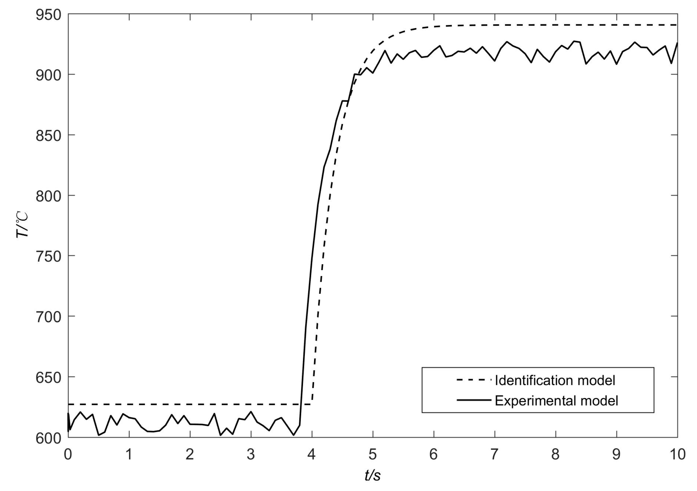
5.2. Experimental Results

To prove the effectiveness of the identification method put forward in this article, the experimental study was carried out. The experimental process is that: firstly, starting the system, and the gas temperature and fuel flow-rate of the HHHTS are controlled at a steady state value. Then, changing the value of fuel flow-rate to realize the value change of gas temperature, and the value of fuel flow-rate and gas temperature are collected in this process, so a set of input and output data of the system are obtained. Finally, an identification model of the gas temperature can be obtained by using the method designed in this paper. In addition, in the experiment, in order to reduce the measurement error, we chose the K-type thermocouple that conforms to the national Class I accuracy standard, and its error was ± 0.4%. The identification model of the gas temperature can be expressed by Equation (29).

$$G_3(s)=\frac{5368}{3.19s+8.56}{e}^{-4s}$$

(29)

It can be seen from Equation (29) that there was a big error between the mathematical model of gas temperature identified by sample data and the mathematical model established by first principle modeling method. The error of $K_p$ was 4.99%, the error of $T_p$ was 18.41%, the error of $a$ was 29.14%, and $\tau$ was within the intended range. This indicates that it is difficult to obtain a precise model of the HHHTS by using first principle modeling method.

To prove the accuracy of the model described by Equation (29), and the output of the identification model was compared with that of the actual system under the same input, so the step response data of the actual system needs to be collected. Since the system will have a large temperature impact when it is just started, the step response data of the system should be collected after the system enters the steady state working condition. In the experiment, firstly, the input fuel flow rate was set to 1 L/min, and then it was adjusted to 1.5 L/min after the gas temperature of the system was stable; finally, the step response data of gas temperature were obtained. To facilitate comparison, the step response curves of the experimental model and the identification model were plotted on a figure, as shown in Figure 8. It can be seen from the figure that the step response curves of the two models were close, and the error of the two models after stabilization was about 2.5%. Therefore, the mathematical model of gas temperature established by the modeling method proposed in this paper had high accuracy, and the mathematical model established can be used for the control of gas temperature.

5.3. Analysis of the Differences

The differences between this paper and other works are shown in the following aspects. First, the object of this paper is HHHTS, which is a high-speed hot wind tunnel and belongs to the combustion field; at present, no one has used gray box modeling to model its gas temperature. Second, although the grey box modeling method adopted in this paper has been applied in many fields, it seems to not be new, but the difference between this paper and other works is that different methods were used to identify different types of parameters, and a new grey box modeling model is proposed, that is, after completing the first principle modeling, according to the characteristics of the parameters to be identified, the recursive least squares method with auxiliary variables and correlation analysis method were used to identify uncertain parameters and time delays, respectively. Finally, in the field of high-speed combustion, CFD is generally used to establish the distributed parameter model of gas temperature in the combustor. This paper attempted to establish the lumped parameter model of gas temperature and study the problem from different angles, which is also the reason why the results of this paper were not obtained by CFD. In a word, the obtained results of this paper are different from other works, in terms of research objects, research questions, and research methods, and had certain innovation and value.

6. Conclusions

To obtain a precise lumped parameter model of gas temperature for a HHHTS, a grey box modeling method was proposed in this paper, which combined first principle modeling method and recursive least squares with auxiliary variables. The following conclusions are drawn through theoretical analysis, simulation, and experimental research.

(1)

The combustion process of the HHHTS is very complicated. Therefore, it is difficult to establish a precise mathematical model of gas temperature by using the first principle modeling method and the system identification modeling method alone.

(2)

The simulation and experimental results show that the grey box modeling method proposed in this paper is feasible, the mathematical model of gas temperature established by the modeling method proposed in this paper has high accuracy, and the mathematical model established can be used for the control of gas temperature.

Although the method proposed in this paper is aimed at modeling the gas temperature of HHHTS, it is a general modeling method that can be easily used for modeling other complex objects with similar characteristics (parameter time-varying, time delay). The basic method is as follows: first, the first principle modeling is applied to establish a preliminary model of the object, and then the input and output data are obtained through experiments on the research object; finally, the recursive least square method with auxiliary variables is used to identify the uncertain parameters of the object, and the time delay of the object is obtained by using the correlation analysis method, so as to finally establish the mathematical model of the object.

References

1. Huang, Q. Future research of the hypersonic and space vehicle technology. Sci. Technol. Inf. 2017, 15, 76–77+79. [Google Scholar]
2. Cai, C.; Yang, Y.; Liu, T. Coordinated control of fuel flow-rate for a high-temperature high-speed wind tunnel. Proc. Inst. Mech. Eng. Part G J. Aerosp. Eng. 2016, 230, 2504–2514. [Google Scholar] [CrossRef]
3. Cai, C.; Li, Y. Undisturbed switching control of fuel flow-rate for a high-speed heat-airflow wind tunnel. Proc. Inst. Mech. Eng. Part G J. Aerosp. Eng. 2014, 228, 2245–2254. [Google Scholar] [CrossRef]
4. Wu, H.; Yu, Y.; Xu, X. Study on identification and modeling of multi-input and multi-output thermal system. J. Chin. Soc. Power Eng. 2010, 30, 196–200. [Google Scholar]
5. Cai, C.; Yang, Y.; Liu, T. Modeling of fuel supply system for a high-temperature high-speed wind tunnel. Adv. Mech. Eng. 2016, 8. [Google Scholar] [CrossRef] [Green Version]
6. Wang, S. Generic modeling and control of an open-circuit piston pump—Par-t I: Theoretical model and analysis. J. Dyn. Sys. Meas. Control 2016, 138, 041004. [Google Scholar] [CrossRef]
7. Wolff, S.; King, R. An annular pulsed detonation combustor mockup: System identification and misfiring detection. J. Eng. Gas Turbines Power 2015, 138, 041603. [Google Scholar] [CrossRef]
8. Mohammadi, E.; Montazeri-Gh, M. A new approach to the gray-box identification of wiener models with the application of gas turbine engine modeling. J. Eng. Gas. Turbines. Power 2015, 137, 071202. [Google Scholar] [CrossRef]
9. Barzegari, M.M.; Alizadeh, E.; Pahnabi, A.H. Grey box modeling and model predictive control for cascade-type PEMFC. Energy 2017, 127, 611–622. [Google Scholar] [CrossRef]
10. Zhao, P.; Wang, S. Gray box modeling of hydraulic servo system based on ODE parameter identification. Hangkong Xuebao/Acta Aeronaut. Et Astronaut. Sin. 2013, 34, 187–196. [Google Scholar]
11. Bidarvatan, M.; Thakkar, V.; Shahbakhti, M.; Bahri, B.; Abdul, A. Grey box modeling of HCCI engines. Appl. Therm. Eng. 2014, 70, 397–409. [Google Scholar] [CrossRef]
12. Farooq, A.A.; Afram, A.; Schulz, N.; Janabi-Sharifi, F. Grey box modeling of a low pressure electric boiler for domestic hot water system. Appl. Therm. Eng. 2015, 84, 257–267. [Google Scholar] [CrossRef]
13. Kicsiny, R. Grey box model for pipe temperature based on linear regression. Int. J. Heat Mass Transf. 2017, 107, 13–20. [Google Scholar] [CrossRef]
14. Shan, D.; Zhang, P.; Wu, Y. Simulation of parameter identification for gun control system based on RLS. J. Syst. Simul. 2013, 25, 1726–1729. [Google Scholar]
15. Hou, Y.; Xue, J.; Wang, L.; Wang, Z. Recursive instrumental variable estimation algorithm for ammonia flow model in SCR denitration reactors. Therm. Power Gener. 2015, 44, 75–80. [Google Scholar]
16. Sun, L.; Yan, Y.; Niu, Y.; Li, Q. Method to identification of system with low order plus time delay. J. North China Electr. Power Univ. 2006, 33, 42–44. [Google Scholar]
Figure 1. The main structure of the system.
Applsci 12 12883 g001
Figure 2. Identification curves of a 1 .
Applsci 12 12883 g002
Figure 3. Identification curves of b 1 .
Applsci 12 12883 g003
Figure 4. The identified object and the identification model.
Applsci 12 12883 g004
Figure 5. Cross correlation function of input and output signals.
Applsci 12 12883 g005
Figure 6. Physical picture of the HHHTS.
Applsci 12 12883 g006
Figure 7. Experimental equipment.
Applsci 12 12883 g007
Figure 8. Step response curves of the two models.
Applsci 12 12883 g008