Article

Quality Assessment of Dual-Parallel Edge Deblocking Filter Architecture for HEVC/H.265

by
Prayline Rajabai Christopher
* and
Sivanantham Sathasivam
*
School of Electronics Engineering, Vellore Institute of Technology, Vellore 632014, Tamil Nadu, India
*
Authors to whom correspondence should be addressed.
Appl. Sci. 2022, 12(24), 12952; https://doi.org/10.3390/app122412952
Submission received: 14 October 2022 / Revised: 12 December 2022 / Accepted: 12 December 2022 / Published: 16 December 2022
(This article belongs to the Special Issue Advance in Digital Signal, Image and Video Processing)

Abstract

:
Preserving the visual quality is a major constraint for any algorithm in image and video processing applications. AVC and HEVC are the extensively used video coding standards for various video processing applications in recent days. These coding standards use filters to preserve the visual quality of the processed video. To retain the quality of the reconstructed video, AVC uses an in-loop filter, called the deblocking filter, while HEVC uses two in-loop filters, the sampling adaptive offset filter and the deblocking filter. These filters are implemented in hardware by adopting various optimization techniques such as reduction of power utilization, reduction of algorithm complexity, and consuming lesser area. The quality of the reconstructed video should not be impacted by these optimization measures. For the HEVC/H.265 coding standard, a parallel edge deblocking filter architecture is designed, and the effectiveness of the parallel edge filter architecture is evaluated using various quantization values for various resolutions. The quality of the parallel edge filter architecture is on par with the HEVC reference model.

1. Introduction

Video compression is ineluctable in recent days owing to the rapid advancements in digital electronics. Several video coding techniques are widely used to compress video data, save storage space, and reduce channel bandwidth during transmission. HEVC is the last released video coding standard developed by the Joint Collaborative Team on Video Coding (JCT-VC) which has been used for more than half a decade in many multimedia applications. This video coding standard splits the raw input video frames into rectangular blocks which are transformed to the frequency domain and then predicted based on the former decoded video either by motion compensated prediction, interprediction, or intraprediction [1]. Due to this block-based transform coding followed by coarse quantization, there may not be uniformity in the intensity of the pixel transition within the two adjacent blocks. This nonuniformity in the transition of the intensity of the pixel values generates a visible discontinuity in the reconstructed video and, thus, degrades the quality of the decoded video.
Nonsmooth block boundaries commonly observed in earlier video coding standards performed at low and medium bit rates, such as visible block boundaries, color biases, and blurring effects [2], still exist in H.264 and H.265. Nonsmooth block boundaries are known as the blocking effect which is one of the most perceivable and objectionable artifacts of block-based compression methods [3,4]. Figure 1 shows the existence of blocking artifacts at the block boundary. It shows the variation of the pixel intensities between the edges of two 4 × 4 blocks. DBFs are used to reduce these blocking artifacts. Figure 2 shows the elimination of the blocking artifacts by smoothening the intensities of the pixels at the edges of a block. The computational complexity of the DBF algorithm is one-third of the H.264 video decoder [3] and one-fifth of the H.265 video decoder [5].
The discontinuities are perceivable for the human visual system (HVS) as blocking effects in the region with lower activity in the video frame [6]. Preserving the same visual quality as the original visual scene is a significant challenge. The AVC and HEVC coding standards utilize lossy compression algorithms such as DCT/DWT, and, hence, the originality of the pixel intensities are lost when the video data are reconstructed. However, measures are taken to upgrade the quality of the reconstructed video in the codec. AVC has an in-loop filter called the deblocking filter (DBF) to reduce visible discontinuities. HEVC standard reduces this visible discontinuity in the main profile by the use of two in-loop filters applied to the reconstructed video in succession. These two in-loop filters are the DBF and the sample adaptive offset (SAO) filter. Although these filters are employed to improve the reconstructed video’s quality, these enhancement methods do not produce a perfect replica of the original image.
The DBF and SAO filters used in HEVC are optimized by modifying the filtering algorithms or by implementing the algorithms efficiently in hardware concerning cost and energy saving. Even though these optimization techniques enhance the quality of the video, we need to measure the quality to compare with different optimization techniques.

2. Related Work on Deblocking Filters

The deblocking filter and the sample adaptive offset (SAO) filter are the two filters used within the codec in the HEVC coding standard. To enhance the visual quality of the reconstructed frames, these filters are applied in two phases, the first stage applying the deblocking filter and the second stage applying the SAO filter. Blocking artifacts are eliminated by the deblocking filter, and the SAO filter enhances the visual quality by adding the offset values to the first-stage filtered pixel samples [7]. Edge offset or band offset are two possible offset values. The two filters for the HEVC coding standard are implemented in hardware adopting several architectural optimization techniques.
The SAO filter and deblocking filter are combined and implemented in hardware, or these filters are implemented separately as deblocking filter [2,8,9,10,11,12,13,14] and SAO filter [15]. Parallel and pipeline-based architectures are utilized to implement the area and throughput optimized deblocking filter. Few deblocking filter architectures use novel ordering for the filtering process to improve the performance. Several filter architectures were implemented by [8,16,17,18,19,20,21,22,23] to realize the H.265 deblocking filter. The deblocking filter architecture of H.264 is more complex compared to the deblocking filter architecture of H.265/HEVC deblocking filter [24]. SAO and deblocking filters were combined and are implemented by [17,23,25,26,27]. In [22,28], a graphics processing unit (GPU) was used to implement the in-loop filter using parallelism. A multicore coprocessor was used to implement the HEVC in-loop filtering in [19]. Convolutional neural network (CNN) was used by [29,30] to create an in-loop deblocking filter with coding unit categorization.

3. Quality Assessment Metrics

The HEVC standard is known to be advantageous for higher video resolutions such as HD and UHD videos with lower bit rates. The features of HEVC improve the compression ratio by 50% with an increase in the complexity by 150% compared to its former video coding standard AVC [31]. Research is ongoing to reduce the overall complexity of the coding standard without affecting the compression ratio. Overall complexity can be reduced if there is a reduction in the complexity of the various modules used in these coding standards, but reduction in computational complexity may deteriorate the quality of the encoded video stream.
Mean square error (MSE) and PSNR are the metrics used to evaluate the objective perceptional video quality [32,33]. Structural similarity (SSIM) is also employed to evaluate the video quality by [34,35], but none of the metrics correlate precisely with the perceptional quality of the HVS [36]. However, SSIM provides better results with respect to the perceptional quality of the HVS using the assessment of three components, viz., perceptional impact of changes in the luminance, contrast, and structure [37]. Despite the complexity of measuring SSIM, due to the assessment of three different components, it is more reliable compared to other measures [38]. Several block-edge impairment metrics were proposed and a generalized block-edge impairment metric (DBIM) was proposed by [39], which shows the difference in the perceptual quality. Equations (1)–(3) show the quality assessment of the reconstructed video using P S N R , M S E , and S S I M , respectively.
M S E i , j = ( i = 1 M j = 1 N [ f i , j F i , j ] 2 ) M . N
P S N R = 20 l o g 10 255 M S E
where f ( i , j ) is the pixel value at ith row and jth column of the original video frame, F ( i , j ) is the pixel value at ith row and jth column of the reconstructed/modified video frame, and M and N represent the width and the height of the video frame. The value of P S N R ranges from 30 dB to 40 dB as the quality of the modified video ranges from medium to high, respectively.
S S I M = ( 2 x ¯ y ¯ + C 1 ) ( 2 σ x y + C 2 ) [ x ¯ 2 + y ¯ 2 + C 1 ] ( σ x 2 + σ y 2 + C 2 )
where x ¯ , y ¯ are the mean of x and y, respectively; σ x , σ y , and σ x y are the variance of x, the variance of y, and the covariance of x and y, respectively; and C 1 and C 2 are constants. S S I M values range between −1 to 1, and the quality is said to be the best when the value is 1 [38].
Among the various metrics for video quality assessment, PSNR is the most desired quality assessment metric owing to its lucidity. Though PSNR is used to check the quality of the video to a great extent, it does not provide the actual perceptual quality as perceived by the HVS.

4. Parallel Edge Deblocking Filter Architecture (PEDBF)

The dual-parallel edge DBF architecture [40], employing five pipeline stages (V-DPEDBF) used to assess the quality, is shown in Figure 3. The (i) control unit, (ii) boundary Strength (BS) calculation unit, and (iii) filter unit are the three main modules in this architecture. The various operations of the filter architecture are administered by the control unit. An enable signal is used as a primary input from the external world to enable the control unit. The control unit oversees and coordinates a number of processes, including data fetch from the external storage, data fetch from the memory within PEDBF, data write to the PEDBF memory, data write to the external storage device, activation of the boundary strength calculator, and activation of the filter unit. The BS unit determines the values of the BS, which range from 0 to 2. The filter unit performs the filtering procedure in accordance with the computed BS value.

4.1. Control Unit

The control unit is activated by the control signal, which is one of the primary inputs to the filter architecture. The control unit of the HEVC DBF has a finite state machine to administer all the operations to handle the deblocking filtering process. When the control signal is not active, all the filtering process is deactivated and, thus, the modules are turned off. Hence, the DBF architecture consumes less power. When the enable signal is active, the control unit triggers the state machine and activates the filtering process in five stages. Five stages—memory read, parameter computation, filter determination, filtering, and memory write—are managed by the state machine during the filtering process. The pixel data are fetched from the external memory, which is outside the filter architecture, after the finite state machine is enabled. Then, 4 × 4 blocks (128 bits) of pixel data are fetched for each clock cycle from the external memory. Figure 4a depicts the sequencing of data fetch from the external memory for a largest coding unit (LCU), which is a 64 × 64 block, whereas Figure 4b,c depict the sequencing of data fetch from the external storage for a 16 × 16 block. The state machine activates the filter unit and the BS calculation unit by generating control signals once four 4 × 4 blocks of pixel data are in place.
The 16 × 16 luma block’s vertical edges V1 and V2 are filtered in parallel in accordance with the determined BS value. Blocks 1 through 8 of the filtered pixel data are then transposed and stored in the internal memory. The filter unit is triggered once more to filter the edges V3 and V4 once the twelfth block of data is accessible. Blocks 9 through 16 of the vertically filtered data are eventually transposed and stored within the PEDBF architecture. After vertical filtering, the horizontal filter is applied by reading the pixel data that are stored within the PEDBF. The internal RAM receives the appropriate signals from the control unit to perform the required operation. H1 and H2 horizontal edges are parallel-filtered and then the filtered data are transposed. The frame memory, which is located external to the architecture, is subsequently written with the filtered data. The horizontal edges H3 and H4 are parallel filtered in a similar manner. After that, they are written to the external frame memory after being transposed. The Chroma Cb and Cr blocks filter the vertical edges (V5 and V6) first, followed by the horizontal edges (H5 and H6) using the same process. The filtered pixel data are subsequently saved in the external storage as 4 × 4 blocks, i.e., 128 bits for each clock cycle.

4.2. Boundary Strength Computation Unit

The boundary strength computation unit computes the BS value, as shown in Figure 5. The BS value range for the HEVC coding standard is between 0 and 2. The BS processing unit receives control signals regarding the pixel block received from the external buffer, such as whether the received pixel block is the left, right, top, or bottom edge of the frame, if it is inter/intracoded, and if its transform coefficients are not zero. The BS value is 0 if the block of pixel data read from the external buffer is a part of the left or top edge of a frame. In addition, the BS value is 0 if the data are not a part of the left or top edge of a frame, the two neighboring 8 × 8 blocks are not intracoded, if the block has nonzero transform coefficients, and if the motion vector is less than 4. The BS value is 1 if the transform coefficients of the block are nonzero and the adjacent blocks are not intracoded. The BS value is also 1 if the adjacent blocks are not intracoded and if the block does not have nonzero transform coefficients, and if the motion vector is higher than or equal to 4. The BS value is 2 if any of the above conditions are not met. DBF is triggered based on the calculated BS value. If the generated value of BS is 0, no filtering is performed; if the determined value is 1, a weak/normal filter is used; and if the stipulated value is 2, a strong filter is used.

4.3. Filter Module

When the pixel data are ready to carry out the filtering operation, the control unit turns on the filter unit. This unit is the sophisticated computational unit. The architecture of the filter unit is shown in Figure 6. It has a parameter computation unit, buffers to store the pixel data, a filter decision block, internal memories, a strong filter, and a weak filter.

4.3.1. Parameter Calculation Unit

This unit calculates the filtering parameters such as β and t c according to Tables 8–12 of [41]. Based on the quantization parameter values and the BS of the neighboring P block and Q block, referred to Q P p and Q P q , respectively, these filtering parameters are calculated. The LUT used to implement the parameter calculation unit has the outputs t c and β . These output values are relative to the inputs BS, Q P p and Q P q .

4.3.2. Buffers

The filter unit of the dual-edge deblocking filter architecture uses eight buffers, as shown in Figure 7, each of which can store a 4 × 4 block of pixels (128 bits). These buffers are initialized with all zeroes. Before the control unit begins the filtering process, the block of pixels 1–4 indicated in Figure 4b from the external memory are stored into the corresponding buffers Q1 BUF, Q2 BUF, Q3 BUF, and Q4 BUF. The filtering operation is carried out along the vertical edges V1 and V2; at the same time, the block of pixels 5–8 is sent to the buffers P1 BUF, P2 BUF, P3 BUF, and P4 BUF, respectively. Figure 8 indicates the relative buffer for both the luma and chroma blocks, along with the outline of each 4 × 4 pixel block. The filtered data are saved to the internal RAM after the edges V1 and V2 have been filtered. Similar techniques are used to filter V3 and V4 vertical edges. For horizontal filtering, the pixel data kept in the internal memory were subsequently transferred to these storage units. The same process is utilized for horizontal filtering as for vertical filtering.

4.3.3. Filter Decision Unit

Based on the values of the parameters β and t c , the strength of the filtering procedure to be used for a 4 × 4 pixel block is determined. The pixel threshold values for the two neighboring blocks are decided by the filter decision unit.

4.3.4. Internal Memories

The memories utilized within the filter architecture employ four dual-port RAM to store the pixel data filtered vertically. A 4 × 4 block of pixel data can be stored in each of the four segments of the 64-byte RAM (16 bytes or 128 bits). Figure 9 and Figure 10 depict the transfer of the pixel data for the luma and the chroma Cb, Cr blocks from the RAM to the buffers. The amount of external memory access cycles is reduced by this method of data storage. It also avoids the utilization of transpose buffers. The first two memory regions are used exclusively during the chroma block filtering procedure, leaving the other regions unused.

4.3.5. Filter Modules

The architecture includes filter modules that make use of both strong and weak/normal filters. Any of these filters are activated according to the filtering decisions determined by the filter decision unit. Therefore, any one of the weak filter or the strong filter is activated to execute the filtering process. The filtering process is omitted if the filtering decision unit determines for no filtering. The weak or strong filtering is executed according to the filtering equations specified in [41]. The similarities in these equations allow for the creation and implementation of a resource-sharing architecture for the filter module, which optimizes the area. The data from the horizontally filtered pixel block are then saved in the external memory, while the data from the vertically filtered pixel block are stored in the internal memory.

4.4. Resource Sharing Architecture

Depending on the deblocking filtering technique used in [9], which follows the HEVC standard, the weak and strong filter units are implemented. The filter architecture is constructed in such a way that it shares the common resources that are used in these equations by taking advantage of the similarity in the filtering equations. This technique thenceforward brings down the area and the power utilization. The pixels of the two neighboring blocks are updated for the strong filter using the third parameter of the clip3 function, which is an equation involving two or more of the pixel values of the adjacent P and Q blocks. Adders and shifters are utilized to implement these equations in the hardware. It is identified that p 0 + q 0 is employed in all the expressions and p 0 + q 0 + 2 is used in most of the expressions. In addition, p 1 + 2 and q 1 + 2 are used twice. Hence, to add p 0 + q 0 , an eight-bit binary adder is employed and the output is fanned out to all the equations. This adder’s output is also used as an input for another binary adder, whose other input is 2, producing the result p 0 + q 0 + 2 , which is then utilized in the appropriate expressions. The same mechanism is used to implement the addition operations p 1 + 2 and q 1 + 2 , and the output of these adders is reused wherever necessary. As a result, the shared resources are distributed over several equations, and an area-optimized filter is used. Figure 11 depicts the resource sharing architecture used for the third argument of the clip3 function for the strong filter.

5. Quality of PEDBF for HEVC/H.265

The optimization techniques employed in the hardware architectures of the DBF filter should not deteriorate the quality of the reconstructed video for any reason. Degradation in the quality of the filtered video will lead to poor performance and coding inefficiency. The DBF algorithm is highly adaptive and data-dependent, as the current edge to be filtered depends on the previously filtered pixel blocks. Since different filter ordering is followed, these changes in the ordering should not affect the quality of the filtered video. Hence, the quality assessment of the dual-edge DBF for H.265 coding standard is measured using PSNR.

Quality Assessment Procedure

To measure the quality of the V-DPEDBF architecture, the following steps are executed sequentially.
  • Original raw video is given as input to the HEVC Test Model to obtain the reconstructed video by disabling the in-loop filter
  • Reconstructed video data from the HM is given as input to the dual-parallel edge deblocking filter (PEDBF) architecture.
  • The input video to PEDBF architecture is split into luminance (Y), chrominance Cb (U) and, chrominance Cr (V) components.
  • Each video component is segregated into image frames and stored into frame buffers.
  • Each image frame of the Y, U, and V components is fetched from the frame buffers.
  • Each image frame is split into uniform pixel blocks of size 16 × 16.
  • Each 16 × 16 block is again split into four 8 × 8 blocks.
  • DBF is applied at the boundary of two 8 × 8 blocks simultaneously for vertical filtering.
  • The vertically filtered output data are transposed and moved into pixel buffers to perform horizontal edge filtering.
  • Horizontal edge filtering is performed after the vertical edge filtering is performed for the entire 16 × 16 block.
  • The horizontally filtered output is transposed and stored into the frame buffer.
  • The filtered video of PEDBF is reconstructed from the frame buffer.
  • The PSNR of the filtered video is computed.
  • Original raw video is given as input to the HEVC Test Model to obtain the reconstructed video by enabling the in-loop filter.
  • The PSNR of the filtered video from the HEVC reference software is computed and the results are compared.
The flow diagram to perform the quality assessment is shown in Figure 12.

6. Filter Selection

The filter architecture uses four resource sharing edge filters that operate simultaneously to filter the edges of two 8 × 8 blocks of pixels. Each 8 × 8 block’s filtering decision is made in accordance with the β , t c parameters and in accordance with the threshold values of the two adjacent pixel blocks. The following criteria are employed for selecting the type of filter:
  • If the BS value is zero, then no filtering is performed.
  • If the BS value is nonzero, then Equations (4)–(8) are computed; and if Equation (8) is not satisfied, then no filtering is performed.
    d p 0 = a b s ( p 2 , 0 2 p 1 , 0 + p 0 , 0 )
    d p 3 = a b s ( p 2 , 3 2 p 1 , 3 + p 0 , 3 )
    d q 0 = a b s ( q 2 , 0 2 q 1 , 0 + q 0 , 0 )
    d q 3 = a b s ( q 2 , 3 2 q 1 , 3 + q 0 , 3 )
    d p 0 + d p 3 + d q 0 + d q 3 < β
  • If Equation (8) is satisfied then Equations (9)–(16) are computed to decide a strong or weak filter. If Equations (11)–(16) are satisfied, then a strong filter is used.
    d p q 0 = d p 0 + d q 0
    d p q 3 = d p 3 + d q 3
    d p q 0 < β / 8
    d p q 3 < β / 8
    a b s p 3 , 0 p 0 , 0 + a b s q 0 , 0 q 3 , 0 < β / 8
    a b s p 3 , 3 p 0 , 3 + a b s q 0 , 3 q 3 , 3 < β / 8
    a b s p 0 , 0 q 0 , 0 < 2.5 t c
    a b s p 0 , 3 q 0 , 3 < 2.5 t c
  • If any one of Equations (11)–(16) are not satisfied, then Equations (17)–(20) are computed and if Equation (20) is satisfied, a weak filter is used.
    d p 0 + d p 3 < β / 16
    d q 0 + d q 3 < β / 16
    δ 0 = 9 q 0 , 0 p 0 , 0 3 q 0 , 1 p 0 , 1 4
    a b s δ 0 < 10 t c
  • If Equation (20) is not satisfied then the filtering process is skipped (no filter).

7. Filtering Operation

The deblocking filtering operations are performed on the edges of the luma and the chroma Cb and Cr pixel blocks based on the computed boundary strength value. Boundary strength is computed based on the coding information given by the codec.

7.1. Luma Block

A strong filter is used, and up to three pixels on either side of the block edges are adjusted as in Equation (21) to Equation (26) for a luma block if the computed BS value is 2.
p 0 = C l i p 3 ( p 0 2 t c , p 0 + 2 t c , p 2 + 2 p 1 + 2 p 0 + 2 q 0 + q 1 + 4 3 )
p 1 = C l i p 3 ( p 1 2 t c , p 1 + 2 t c , p 2 + p 1 + p 0 + q 0 + 2 2 )
p 2 = C l i p 3 ( p 2 2 t c , p 2 + 2 t c , 2 p 3 + 3 p 2 + p 1 + p 0 + q 0 + 4 3 )
q 0 = C l i p 3 ( q 0 2 t c , q 0 + 2 t c , p 1 + 2 p 0 + 2 q 0 + 2 q 1 + q 2 + 4 3 )
q 1 = C l i p 3 ( q 1 2 t c , q 1 + 2 t c , q 2 + q 1 + q 0 + p 0 + 2 2 )
q 2 = C l i p 3 ( q 2 2 t c , q 2 + 2 t c , 2 q 3 + 3 q 2 + q 1 + q 0 + p 0 + 4 3 )
If BS = 1, then a weak filter is applied and the pixels on either side of the block edges are modified as in Equations (27)–(32).
Δ = 9 q 0 p 0 3 q 1 p 1 + 8 4
If Abs ( Δ ) < 10 t c then
Δ = C l i p 3 ( t c , t c , Δ )
p 0 = C l i p 1 Y ( p 0 + Δ )
q 0 = C l i p 1 Y ( q 0 Δ )
when dEp = 1, then
p 1 = C l i p 1 Y ( p 1 + Δ p )
where Δ p = C l i p 3 ( t c 2 , t c 2 , p 2 + p 0 + 1 1 p 1 + Δ 1 ) .
When dEq = 1, then
q 1 = C l i p 1 Y ( q 1 + Δ q )
where Δ q = C l i p 3 ( t c 2 , t c 2 , q 2 + q 0 + 1 1 q 1 + Δ 1 )

7.2. Chroma Block—Cb and Cr

Chroma blocks are filtered only if BS = 2, and no filtering is performed when BS = 1 or 0. When BS = 2, the strong filter is applied, and the pixels p 0 and q 0 alone on either sides of the block edges are modified as in Equations (33)–(35).
Δ c = C l i p 3 ( t c , t c , ( p 0 q 0 2 + p 1 q 1 + 4 ) 3 )
p 0 = C l i p Y ( p 0 + Δ c )
q 0 = C l i p Y ( q 0 Δ c )

8. Results and Discussion

The quality assessment of the five-stage pipelined dual-edge deblocking filter architecture implemented for the HEVC standard [40] is performed using Matlab. Different test video sequences are used to obtain the PSNR values of the PEDBF architecture using different QP values. The typical QP value is 32. Hence, the quality assessment is performed with the typical QP value (32), the QP value lesser than the typical value (27), and QP value greater than the typical QP (37). Figure 13 shows an image frame of the original video sequence. This original/raw video sequence is given as input to the HM software to obtain two different types of encoded video. One type of encoded video is obtained from the HM software with the deblocking filter turned off (without DBF), and another type of encoded video is obtained from the HM software with the deblocking filter turned on (with DBF). Figure 14 and Figure 15 show a sample frame of the output video sequence from the HM software without DBF and with DBF, respectively. The encoded output video from the HM software without DBF is used to perform the quality analysis of the PEDBF architecture. This video encoded without DBF is given as the input video sequence to the PEDBF implemented in Matlab to undergo deblocking filtering. Figure 16 shows a sample frame of the output video obtained from the PEDBF. The PSNR value of the output video obtained from the PEBDF is computed.
The quality of this architecture is assessed by comparing the PSNR value of the output video of the PEDBF architecture and the PSNR value of the video obtained using the HM software with DBF turned on for different QP values. The results for QCIF video sequences are tabulated in Table 1 and the comparison graph is shown in Figure 17 with QP = 32. The results for CIF video sequences are tabulated in Table 2 and the comparison graph is shown in Figure 18 with QP = 32. It is noted that the implemented architecture shows a slight improvement in quality concerning the PSNR metrics. The execution time for QCIF and CIF video sequences are tabulated in Table 3 and Table 4, respectively, and the comparison graphs are shown in Figure 19 and Figure 20. It is seen that, as the two edges are filtered in parallel, the filtering time is reduced by 50%, and thus the throughput of the architecture is improved by 50% with the increase in quality.
Table 5 and Table 6 show the results of QCIF and CIF video sequences, respectively, filtered with QP = 37, and the comparison graphs are shown in Figure 21 and Figure 22. The execution time for QCIF and CIF video sequences are tabulated in Table 7 and Table 8, and the comparison graphs are shown in Figure 23 and Figure 24.
Table 9 and Table 10 show the results of QCIF and CIF video sequences, respectively, filtered with QP = 27, and the comparison graphs are shown in Figure 25 and Figure 26. The execution time for QCIF and CIF video sequences are tabulated in Table 11 and Table 12, and the comparison graphs are shown in Figure 27 and Figure 28.
Based on the experiments carried out with different video sequences of different resolutions for different QP values, it is identified that as the QP value increases, the quality decreases and results in lower PSNR values. In addition, the execution time decreases as the QP value increases. This behavior is as expected with any video coding algorithm. Hence, the PEDBF architecture complies with the coding standards. The execution time of the PEDBF architecture is reduced to almost half of the execution time of the HM, owing to the fact of filtering two edges in parallel.

9. Conclusions

The quality assessment of any algorithm implemented in hardware is strongly required as the optimization techniques do not affect the quality of the reconstructed video data in any of the processing steps. Among the various quality assessment metrics, we use the metric PSNR to assess the quality of the video owing to its simplicity. Raw video data of two different resolutions (QCIF and CIF) are taken and the quality of the filtered video is checked with the quality of the video obtained from the HEVC Test Model. It is noted that the quality of the parallel edge filter architecture does not affect the quality of the reconstructed video, and it shows slight improvements compared to the HEVC Test Model. In one second, ten to twelve separate images can be processed by the human visual system by perceiving each image discretely. One image is held in the visual cortex for around one of fifteen parts in a second. Therefore, as the frame rate is higher, perception of the moving picture will be smooth. Hence, the processing time decreases in the dual-parallel edge DBF, the frame rate will increase, and, thus, the perceptual quality is increased.

Author Contributions

Conceptualization, P.R.C. and S.S.; methodology, P.R.C. and S.S.; validation, P.R.C.; formal analysis, P.R.C.; investigation, P.R.C. and S.S.; resources, P.R.C.; data curation, P.R.C.; writing—original draft preparation, P.R.C.; writing—review and editing, P.R.C. and S.S.; supervision, S.S. All authors have read and agreed to the published version of the manuscript.

Funding

The APC is funded by Vellore Institute of India, Vellore, Tamil Nadu, India.

Institutional Review Board Statement

Not applicable.

Informed Consent Statement

Not applicable.

Data Availability Statement

The reference software for HEVC called HM (HEVC Test Model) is from HM software repository https://hevc.hhi.fraunhofer.de/svn/svn_HEVCSoftware (accessed on 1 October 2022), and the test video sequences used for quality assessment are from the Video Trace Library of Arizona State University http://trace.eas.asu.edu/yuv/index.html (accessed on 1 October 2022) and Video Information Processing Lab of National Chiao Tung University http://vip.cs.nctu.edu.tw/resource_seq.html (accessed on 1 October 2022).

Acknowledgments

The authors would like to acknowledge Vellore Institute of Technology, Vellore, Tamil Nadu, India, for providing all the necessary facilities for the research.

Conflicts of Interest

The authors declare no conflict of interest.

References

  1. Wedi, T.; Musmann, H.G. Motion-and aliasing-compensated prediction for hybrid video coding. IEEE Trans. Circuits Syst. Video Technol. 2003, 13, 577–586. [Google Scholar] [CrossRef] [Green Version]
  2. Zhou, W.; Zhang, J.; Zhou, X.; Liu, Z.; Liu, X. A high-throughput and multi-parallel VLSI architecture for HEVC deblocking filter. IEEE Trans. Multimed. 2016, 18, 1034–1047. [Google Scholar] [CrossRef]
  3. Pourazad, M.T.; Doutre, C.; Azimi, M.; Nasiopoulos, P. HEVC: The new gold standard for video compression: How does HEVC compare with H. 264/AVC? IEEE Consum. Electron. Mag. 2012, 1, 36–46. [Google Scholar] [CrossRef]
  4. Singh, J.; Singh, S.; Singh, D.; Uddin, M. Blocking artefact detection in block-based DCT compressed images. Int. J. Signal Imaging Syst. Eng. 2011, 4, 181–188. [Google Scholar] [CrossRef]
  5. Vanne, J.; Viitanen, M.; Hamalainen, T.D.; Hallapuro, A. Comparative rate-distortion-complexity analysis of HEVC and AVC video codecs. IEEE Trans. Circuits Syst. Video Technol. 2012, 22, 1885–1898. [Google Scholar] [CrossRef]
  6. Tai, S.C.; Chen, Y.Y.; Sheu, S.F. Deblocking filter for low bit rate MPEG-4 video. IEEE Trans. Circuits Syst. Video Technol. 2005, 15, 733–741. [Google Scholar]
  7. Wang, Y.; Guo, X.; Lu, Y.; Fan, X.; Zhao, D. GPU-based optimization for sample adaptive offset in HEVC. In Proceedings of the 2016 IEEE International Conference on Image Processing (ICIP), Phoenix, AZ, USA, 25–28 September 2016; pp. 829–833. [Google Scholar]
  8. Li, M.; Zhou, J.; Zhou, D.; Peng, X.; Goto, S. De-blocking Filter Design for HEVC and H. 264/AVC. In Lecture Notes in Computer Science, Proceedings of the 13th Pacific-Rim Conference on Multimedia, Singapore, Singapore, 4–6 December 2012; Springer: Berlin/Heidelberg, Germany, 2012; pp. 273–284. [Google Scholar]
  9. Hsu, P.K.; Shen, C.A. The VLSI Architecture of a Highly Efficient Deblocking Filter for HEVC Systems. IEEE Trans. Circuits Syst. Video Technol. 2017, 27, 1091–1103. [Google Scholar] [CrossRef]
  10. Ye, X.; Ding, D.; Yu, L. A cost-efficient hardware architecture of deblocking filter in HEVC. In Proceedings of the Visual Communications and Image Processing Conference, Valletta, Malta, 7–10 December 2014; pp. 209–212. [Google Scholar]
  11. Bae, J. Register array-based VLSI architecture of H. 265/HEVC loop filter. IEICE Electron. Express 2013, 10, 20130161. [Google Scholar] [CrossRef] [Green Version]
  12. Tang, G.; Zeng, X.; Fan, Y. An SRAM-free HEVC Deblocking Filter VLSI Architecture for 8K Application. In Proceedings of the 2018 14th IEEE International Conference on Solid-State and Integrated Circuit Technology (ICSICT), Qingdao, China, 31 October–3 November 2018; pp. 1–3. [Google Scholar] [CrossRef]
  13. Peesapati, R.; Das, S.; Baldev, S.; Ahamed, S.R. Design of streaming deblocking filter for HEVC decoder. IEEE Trans. Consum. Electron. 2017, 63, 1–9. [Google Scholar] [CrossRef]
  14. Jiang, L.; Yang, Q.; Zhu, Y.; Deng, J. A parallel implementation of deblocking filter based on video array architecture for HEVC. In Proceedings of the 2016 Seventh International Green and Sustainable Computing Conference (IGSC), Hangzhou, China, 7–9 November 2016; pp. 1–7. [Google Scholar] [CrossRef]
  15. Park, S.; Ryoo, K. Hardware design of HEVC in-loop filter for ultra-HD video encoding. Lect. Notes Electr. Eng. 2019, 518, 405–409. [Google Scholar] [CrossRef]
  16. Shen, W.W.; Shang, Q.; Shen, S.; Fan, Y.; Zeng, X. A high-throughput VLSI architecture for deblocking filter in HEVC. In Proceedings of the IEEE International Symposium on Circuits and Systems, Beijing, China, 19–23 May 2013; pp. 673–676. [Google Scholar]
  17. Shen, S.; Shen, W.; Fan, Y.; Zeng, X. A pipelined VLSI architecture for Sample Adaptive Offset (SAO) filter and deblocking filter of HEVC. IEICE Electron. Express 2013, 10, 20130272. [Google Scholar] [CrossRef] [Green Version]
  18. Ozcan, E.; Adibelli, Y.; Hamzaoglu, I. A high performance deblocking filter hardware for high efficiency video coding. IEEE Trans. Consum. Electron. 2013, 59, 714–720. [Google Scholar] [CrossRef]
  19. Hautala, I.; Boutellier, J.; Hannuksela, J.; Silvén, O. Programmable low-power multicore coprocessor architecture for HEVC/H. 265 in-loop filtering. IEEE Trans. Circuits Syst. Video Technol. 2014, 25, 1217–1230. [Google Scholar] [CrossRef]
  20. Yan, C.; Zhang, Y.; Dai, F.; Wang, X.; Li, L.; Dai, Q. Parallel deblocking filter for HEVC on many-core processor. Electron. Lett. 2014, 50, 367–368. [Google Scholar] [CrossRef]
  21. Mody, M.; Nandan, N.; Hideo, T. High throughput VLSI architecture supporting HEVC loop filter for Ultra HDTV. In Proceedings of the 2013 IEEE Third International Conference on Consumer Electronics—Berlin (ICCE-Berlin), Berlin, Germany, 9–11 September 2013; pp. 54–57. [Google Scholar]
  22. Wang, Y.; Guo, X.; Fan, X.; Lu, Y.; Zhao, D.; Gao, W. Parallel In-Loop Filtering in HEVC Encoder on GPU. IEEE Trans. Consum. Electron. 2018, 64, 276–284. [Google Scholar] [CrossRef]
  23. Kim, H.; Ko, J.; Park, S. An Efficient Architecture of In-Loop Filters for Multicore Scalable HEVC Hardware Decoders. IEEE Trans. Multimed. 2017, 20, 810–824. [Google Scholar] [CrossRef]
  24. Kotra, A.M.; Raulet, M.; Deforges, O. Comparison of different parallel implementations for deblocking filter of HEVC. In Proceedings of the 2013 IEEE International Conference on Acoustics, Speech and Signal Processing, Vancouver, BC, Canada, 26–31 May 2013; pp. 2721–2725. [Google Scholar]
  25. Liu, L.; Chen, Y.; Deng, C.; Yin, S.; Wei, S. Implementation of in-loop filter for HEVC decoder on reconfigurable processor. IET Image Process. 2017, 11, 685–692. [Google Scholar] [CrossRef]
  26. Shen, W.; Fan, Y.; Bai, Y.; Huang, L.; Shang, Q.; Liu, C.; Zeng, X. A Combined Deblocking Filter and SAO Hardware Architecture for HEVC. IEEE Trans. Multimed. 2016, 18, 1022–1033. [Google Scholar] [CrossRef]
  27. Baldev, S.; Shukla, K.; Gogoi, S.; Rathore, P.K.; Peesapati, R. Design and Implementation of Efficient Streaming Deblocking and SAO Filter for HEVC Decoder. IEEE Trans. Consum. Electron. 2018, 64, 127–135. [Google Scholar] [CrossRef]
  28. Jiang, W.; Mei, H.; Lu, F.; Jin, H.; Yang, L.T.; Luo, B.; Chi, Y. A novel parallel deblocking filtering strategy for HEVC/H.265 based on GPU. Concurr. Comput. Pract. Exp. 2016, 28, 4264–4276. [Google Scholar] [CrossRef]
  29. Dai, Y.; Liu, D.; Zha, Z.J.; Wu, F. A CNN-Based In-Loop Filter with CU Classification for HEVC. In Proceedings of the 2018 IEEE Visual Communications and Image Processing (VCIP), Taichung, Taiwan, 9–12 December 2018; pp. 1–4. [Google Scholar]
  30. Park, W.S.; Kim, M. CNN-based in-loop filtering for coding efficiency improvement. In Proceedings of the 2016 IEEE 12th Image, Video, and Multidimensional Signal Processing Workshop (IVMSP), Bordeaux, France, 11–12 July 2016; pp. 1–5. [Google Scholar] [CrossRef]
  31. Zuo-Cheng, Z.; Ke-Bin, J. Key technologies and new developments of next generation video coding standard HEVC. In Proceedings of the 2013 Ninth International Conference on Intelligent Information Hiding and Multimedia Signal Processing, Beijing, China, 16–18 October 2013; pp. 125–128. [Google Scholar]
  32. Na, T.; Kim, M. A novel no-reference PSNR estimation method with regard to deblocking filtering effect in H. 264/AVC bitstreams. IEEE Trans. Circuits Syst. Video Technol. 2013, 24, 320–330. [Google Scholar]
  33. Tanchenko, A. Visual-PSNR measure of image quality. J. Vis. Commun. Image Represent. 2014, 25, 874–878. [Google Scholar] [CrossRef]
  34. Ou, T.S.; Huang, Y.H.; Chen, H.H. SSIM-based perceptual rate control for video coding. IEEE Trans. Circuits Syst. Video Technol. 2011, 21, 682–691. [Google Scholar]
  35. Wang, S.; Rehman, A.; Wang, Z.; Ma, S.; Gao, W. Perceptual video coding based on SSIM-inspired divisive normalization. IEEE Trans. Image Process. 2012, 22, 1418–1429. [Google Scholar] [CrossRef] [PubMed]
  36. Winkler, S. Digital Video Quality: Vision Models and Metrics; John Wiley and Sons: Hoboken, NJ, USA, 2005. [Google Scholar]
  37. Dosselmann, R.; Yang, X.D. A comprehensive assessment of the structural similarity index. Signal Image Video Process. 2011, 5, 81–91. [Google Scholar] [CrossRef]
  38. Wang, Y. Survey of Objective Video Quality Measurements. 2006. Available online: https://digitalcommons.wpi.edu/computerscience-pubs/42 (accessed on 10 September 2019).
  39. Wei, W.Y. Deblocking Algorithms in Video and Image Compression Coding; National Taiwan University: Taipei, Taiwan, 2009. [Google Scholar]
  40. Christopher, P.R.; Sathasivam, S. Five-stage pipelined dual-edge deblocking filter architecture for H.265 video codec. IEICE Electron. Express 2019, 16, 20190500. [Google Scholar] [CrossRef]
  41. H.265-ITU-T; SERIES H: Audiovisual and Multimedia Systems—Infrastructure of Audiovisual Services—Coding of Moving Video, High Efficiency Video Coding. Telecommunication Standardization Sector of ITU: Paris, France, 2018; Recommendation ITU-T H.265.
Figure 1. Variation of pixel intensities between block boundaries.
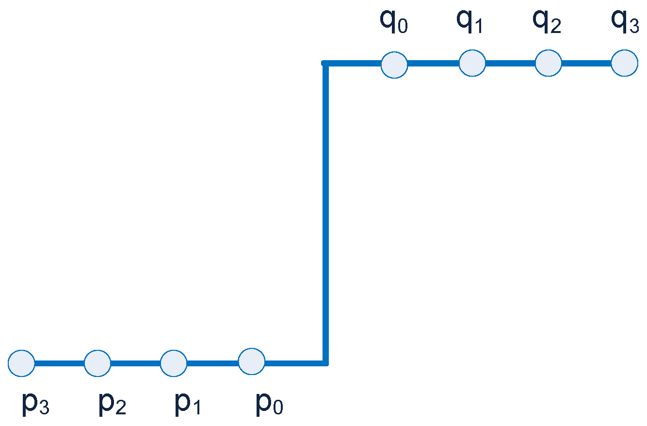
Applsci 12 12952 g001
Figure 2. Smoothing of pixel intensities between block boundaries.
Applsci 12 12952 g002
Figure 3. Architecture of V-DPEDBF for HEVC [40].
Applsci 12 12952 g003
Figure 4. (a) Sequence of read for an LCU; (b,c) sequence of read for a 16 × 16 block.
Applsci 12 12952 g004
Figure 5. Boundary strength computation unit.
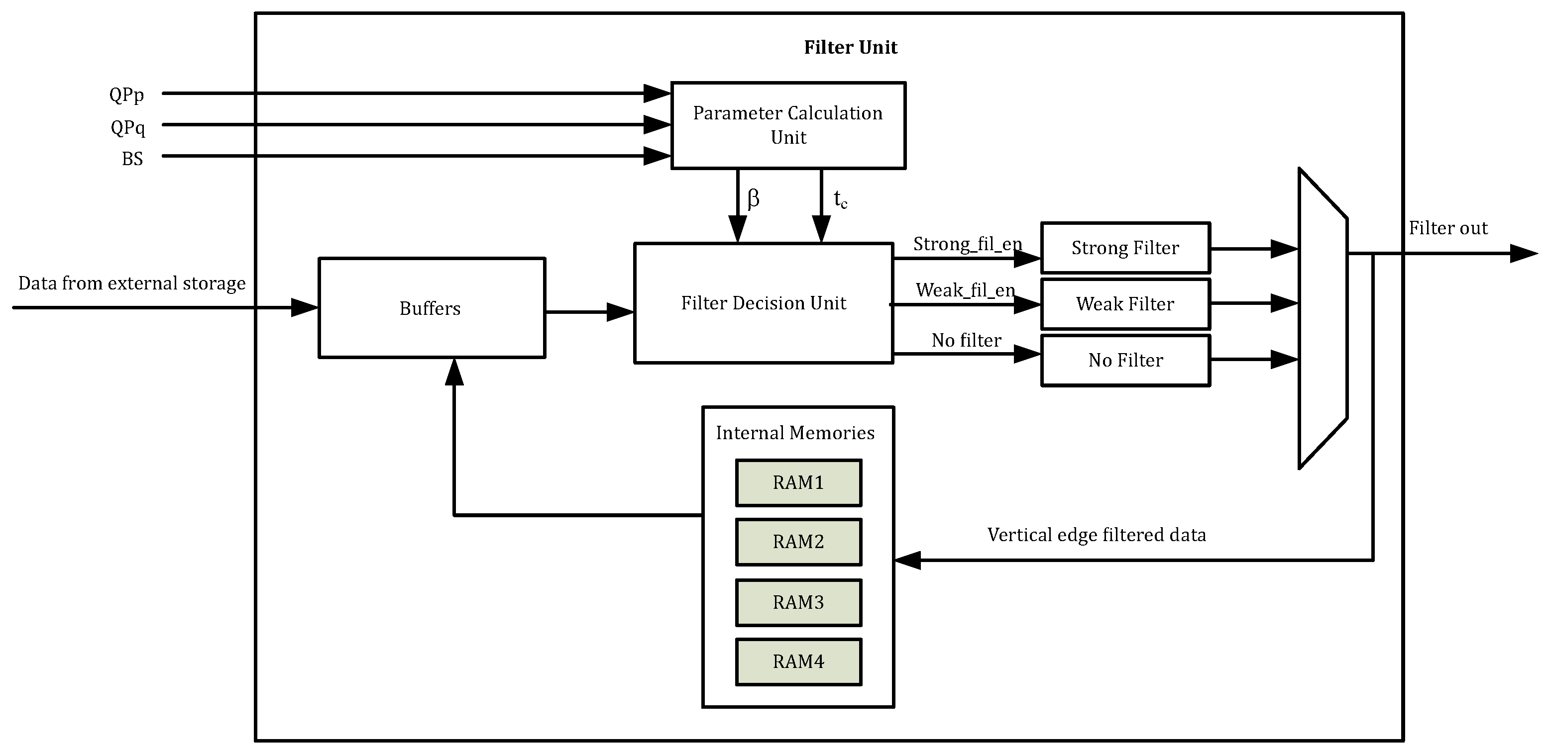
Applsci 12 12952 g005
Figure 6. Filter unit of dual-edge deblocking filter architecture.
Applsci 12 12952 g006
Figure 7. Buffers to store the pixel block.
Applsci 12 12952 g007
Figure 8. Mapping of pixel blocks to buffers: (a) pixel blocks; (b) buffers.
Applsci 12 12952 g008
Figure 9. Mapping of internal memory to buffer before horizontal filtering for luma block.
Applsci 12 12952 g009
Figure 10. Mapping of internal memory to buffer before horizontal filtering for chroma block.
Applsci 12 12952 g010
Figure 11. Resource sharing architecture of strong filter—partial view.
Applsci 12 12952 g011
Figure 12. Flow diagram to perform quality assessment.
Applsci 12 12952 g012
Figure 13. Frame of the original input video.
Applsci 12 12952 g013
Figure 14. Frame of output video from HM with DBF disabled.
Applsci 12 12952 g014
Figure 15. Frame of output video from HM with DBF enabled.
Applsci 12 12952 g015
Figure 16. Frame of output video from dual PEDBF.
Applsci 12 12952 g016
Figure 17. Comparison of PSNR with HM for QCIF video sequences using QP = 32.
Applsci 12 12952 g017
Figure 18. Comparison of PSNR with HM for CIF video sequences using QP = 32.
Applsci 12 12952 g018
Figure 19. Comparison of processing time with HM for QCIF video sequences using QP = 32.
Applsci 12 12952 g019
Figure 20. Comparison of processing time with HM for CIF video sequences using QP = 32.
Applsci 12 12952 g020
Figure 21. Comparison of PSNR with HM for QCIF video sequences using QP = 37.
Applsci 12 12952 g021
Figure 22. Comparison of PSNR with HM for CIF video sequences using QP = 37.
Applsci 12 12952 g022
Figure 23. Comparison of processing time with HM for QCIF video sequences using QP = 37.
Applsci 12 12952 g023
Figure 24. Comparison of processing time with HM for CIF video sequences using QP = 37.
Applsci 12 12952 g024
Figure 25. Comparison of PSNR with HM for QCIF video sequences using QP = 27.
Applsci 12 12952 g025
Figure 26. Comparison of PSNR with HM for CIF video sequences using QP = 27.
Applsci 12 12952 g026
Figure 27. Comparison of processing time with HM for QCIF video sequences using QP = 27.
Applsci 12 12952 g027
Figure 28. Comparison of processing time with HM for CIF video sequences using QP = 27.
Applsci 12 12952 g028
Table 1. PSNR of QCIF video sequences with QP = 32.
Video SequenceHM (dB)PEDBF (dB)
Akiyo37.383337.59186
Coastguard34.413836.40767
Foreman35.427436.58643
Mobile Calendar32.236632.85071
Hall36.433437.235
Carphone36.197236.4323
Miss America38.897239.12775
Table 2. PSNR of CIF video sequences with QP = 32.
Video SequenceHM (dB)PEDBF (dB)
Akiyo38.30773739.2812
Coastguard35.0372334.9852
Foreman35.895135.99
Mobile Calendar33.0441133.0432
Hall36.9320837.4513
Tempete34.0922734.224
Table 3. Processing time of QCIF video sequences with QP = 32.
Video SequenceHM (Sec)PEDBF (Sec)
Akiyo64.67839.4553
Coastguard85.10344.81924
Foreman82.36845.6632
Mobile Calendar85.67343.21693
Hall64.06437.28175
Carphone73.35843.57872
Miss America23.81113.27997
Table 4. Processing time of CIF video sequences with QP = 32.
Video SequenceHM (Sec)PEDBF (Sec)
Akiyo264.989165.49741
Coastguard376.373196.2231
Foreman278.388176.485
Mobile Calendar312.898193.3375
Hall219.416112.2503
Tempete229.776152.46557
Table 5. PSNR of QCIF video sequences with QP = 37.
Video SequenceHM (dB)PEDBF (dB)
Akiyo34.018234.893362
Coastguard31.139233.457211
Foreman32.199733.862149
Mobile Calendar28.318929.568311
Hall32.97134.430916
Carphone32.986534.303814
Miss America36.418537.267113
Table 6. PSNR of CIF video sequences with QP = 37.
Video SequenceHM (dB)PEDBF (dB)
Akiyo36.298536.716387
Coastguard31.804333.970701
Foreman33.005134.390624
Mobile Calendar29.222230.454212
Hall34.543735.553274
Tempete30.682832.131876
Table 7. Processing time of QCIF video sequences with QP = 37.
Video SequenceHM (Sec)PEDBF (Sec)
Akiyo46.35423.904816
Coastguard52.0227.976072
Foreman48.86128.335635
Mobile Calendar70.90538.544973
Hall50.13828.943229
Carphone63.93833.216266
Miss America23.77815.006227
Table 8. Processing time of CIF video sequences with QP = 37.
Video SequenceHM (Sec)PEDBF (Sec)
Akiyo361.664139.577545
Coastguard323.229141.569951
Foreman293.987161.030763
Mobile Calendar461.949225.603688
Hall280.68142.62714
Tempete200.476112.878238
Table 9. PSNR of QCIF video sequences with QP = 27.
Video SequenceHM (dB)PEDBF (dB)
Akiyo40.899940.891213
Coastguard38.167339.927605
Foreman38.929439.793245
Mobile Calendar36.629236.744202
Hall39.873340.164219
Carphone39.661739.917189
Miss America41.571941.766507
Table 10. PSNR of CIF video sequences with QP = 27.
Video SequenceHM (dB)PEDBF (dB)
Akiyo42.286142.332459
Coastguard38.659840.411503
Foreman39.252940.130872
Mobile Calendar37.137837.29197
Hall40.137540.525791
Tempete38.057238.495716
Table 11. Processing time of QCIF video sequences with QP = 27.
Video SequenceHM (Sec)PEDBF (Sec)
Akiyo66.6132.722607
Coastguard72.62739.74846
Foreman81.68141.068033
Mobile Calendar120.71658.555709
Hall67.68735.016408
Carphone95.3455.400211
Miss America24.74113.174376
Table 12. Processing time of CIF video sequences with QP = 27.
Video SequenceHM (Sec)PEDBF (Sec)
Akiyo205.041100.410937
Coastguard277.788150.710927
Foreman250.539126.669947
Mobile Calendar352.151208.336164
Hall228.818117.526938
Tempete263.123156.781587
Publisher’s Note: MDPI stays neutral with regard to jurisdictional claims in published maps and institutional affiliations.

