Abstract
Even though two-phase heat transfer of refrigerants in minichannel heat sinks has been studied extensively, there is still a demand for improvements in overall thermal performance of miniature heat transfer exchangers. Experimental investigation and sophisticated heat transfer calculations with respect to heat transfer devices are still needed. In this work, a time-dependent experimental study of subcooled boiling was carried out for FC-72 flow in a heat sink, comprising of five asymmetrically heated minichannels. The heater surface temperature was continuously monitored by an infrared camera. The boiling heat transfer characteristics were investigated and the effect of the mass flow rate on the heat transfer coefficient was studied. In order to solve the heat transfer problem related to time-dependent flow boiling, two numerical methods, based on the FEM were applied, and based on the Trefftz functions (FEMT) and using the ADINA program. The results achieved with these two calculation methods were explored with an emphasis on the impact of the mass flow rate (range from 5 to 55 kg/h) on the resulting heat transfer coefficient. It was found that, with increasing mass flow, the heat transfer coefficient increased. Good agreement was found between the heat transfer coefficients, determined according to two numerical methods and the simple 1D calculation method.
1. Introduction
Miniature heat exchangers have received considerable attention, given potential for high heat transfer removal and the success of this device in high heat-flux, as developments in electronic equipment with the advent of modern technology. In such devices, a huge amount of heat is produced during their operation, which results in reduced reliability, normal performance, and their prognosed work. Therefore, a proper cooling mechanism is of great importance when designing miniature electronic components. The heat dissipation capabilities associated with minichannel heat sinks have been developed because they have a good potential for effectiveness and are still promising. Quite a few studies have developed various aspects of applications of mini heat exchangers, including theoretical perspectives and practical aspects.
There is still a demand for an improvement in overall thermal performance of miniature heat transfer exchangers when both heat transfer and hydrodynamic characteristics are considered. Currently, heat transfer, with the change of state during flow refrigerants in minichannel heat sinks, has been studied extensively. Meanwhile, only a few studies have been devoted to investigating different methods of heat transfer calculations regarding miniature heat transfer devices, and it remains inconclusive whether similar results are expected. Many recent studies have concentrated on enhancement of heat transfer in minichannel heat sinks. Several of these studies have focused on the effects of heat flux, mass flow rate or fluid velocity, Reynolds number, mass flux, pressure, inlet liquid subcooling, channel dimensions and spatial orientation on improving the cooling performances of miniature heat exchangers.
In the current computational age, heat transfer analysis, using numerical methods, has become a common mode to reduce time, cost, and material. In-depth analysis and study of flow behaviour and pattern in the flow domain can be obtained very quickly with the aid of commercial software and by developing computer codes. Heat transfer analysis in the minichannel heat sink using the numerical method is generally needed to be carried out by either reliable data upload in the calculation methods. However, numerical analysis conducted in commercial software, based on experimental data, is more valuable because it ensures verification of the simulation results.
In this work, an experimental study of subcooled flow boiling was conducted for FC-72 flow in a minichannel heat sink, comprising of five channels. The boiling heat transfer characteristics were investigated, and the effect of the mass flow rate on the heat transfer coefficient was studied. The results achieved on different calculation methods were also explored with an emphasis on the impact of the mass flow rate on the heat transfer intensity. The research reported in the literature confirms the importance of different flow and thermal parameters in the flow boiling heat transfer. Different criteria for predicting the transition from macro-channels to mini-/microchannels were proposed. The classification of channels, taking into account their hydraulic dimension according to Kandlikar and Grande [1], is common, that is, it has been stated that macrochannel in minichannel transition occurs at a hydraulic diameter of 3 mm.
The effect of low heat and mass fluxes on the boiling heat transfer coefficient of R-245fa was examined in [2]. In the test section, a smooth horizontal tube, with an inner diameter of 8.31 mm and a heated length of 0.8 m, was provided. The steady-state experiments were carried out in a wide range of vapour qualities (from 0.05 to 0.90) for mass fluxes of 40, 60 and 80 kg/(m2s) and heat fluxes of 2.5, 5.0 and 7.5 kW/m2. The authors stated that the heat transfer coefficient was influenced by both the mass and the heat fluxes. An increase in the mass flux resulted in an increase in the heat transfer coefficient. The higher vapour quality cases were more sensitive to the mass flux than lower vapour quality cases, except at low heat flux conditions. For all other heat fluxes, the heat transfer coefficient was found to be independent of the vapour quality, except when the mass flux was high, where an increase in the vapour quality resulted in improved heat transfer coefficients.
The authors of [3] focused on experimental boiling heat transfer during the R-245fa flow in a small circular channel. In the test section, there was a horizontal polyimide tube of 2.689 mm inner diameter and 285 mm long, heated by a counter-current water flow in an annulus around the test tube. Mass fluxes ranged from 100 to 500 kg/(m2s) and heat fluxes from 15 to 55 kW/m2. It was noticed that a higher mass flux resulted in a higher heat transfer coefficient. At a mass flux of 100 kg/(m2s), the vapour quality had a negligible effect on the heat transfer coefficient. Heat flux did not have a noticeable effect. Furthermore, the authors claimed that increasing the saturation temperature had an almost negligible effect on the heat transfer coefficient at a mass flux of 200 kg/(m2s) and a heat flux of 15 kW/m2 and at higher mass and heat fluxes the heat transfer coefficient was lowered with increasing temperature.
The works [4,5,6] refer to boiling heat transfer in an asymmetrically heated minichannels. The article [4] describes the results of subcooled flow boiling heat transfer in a group of five 1 mm deep in several spatial orientations. The heat transfer problem was solved using the Trefftz method and the FEM with Trefftz type basis functions. The main objective of [5] was the mathematical modelling of the time-dependent heat transfer processes during FC-72 flow boiling in a minichannel heat sink. Three mathematical methods were applied in the calculations: the FEM with Trefftz type basis functions, the Classical Trefftz Method and the Hybrid Picard-Trefftz Method. The authors of [6] focused on studying boiling heat transfer during the cooling liquid flow (FC-72, HFE-649, HFE-70 00 and HFE-7100), along a single depth of 1.7 mm, vertical or horizontal oriented minichannel. The inverse heat conduction problem in the heated wall was solved by the Finite Element Method with shape functions based on the Hermite interpolation and the Trefftz functions.
There are well-known commercial computational fluid dynamics (CFD) programs. The most popular are the following: ANSYS CFX/Fluent [7,8] and COMSOL Multiphysics [9]. In [7] the authors have considered four-row finned-tube heat exchangers. The main result was the proposition of new correlations for the air-side Nusselt number for the four-row finned tube heat exchanger. ANSYS Fluent software has been used in [8]. The study focuses on comparing experimental heat transfer coefficients on the local air side with numerical results obtained with the help of the ANSYS Fluent software. The authors have achieved good agreement between the heat transfer coefficients obtained from the experimental measurements and the numerical computations. They have found that the agreement decreases as the complexity of the geometry increases. The article [9] concentrates on forced convection with a high Reynolds number of the water-alumina-based nanofluid in the square cavity containing a rotating disk with unit speed. The influence of the rotating disc on the temperature distribution and the value of the Nusselt number has been investigated.
The OpenFOAM and Simcenter STAR-CCM+ software are also mentioned as useful CFD applications. In [10], a wall nucleation model was proposed for subcooled boiling flow in narrow rectangular channels, implemented in a two-phase Eulerian-Eulerian CFD model, using the OpenFOAM platform, utilizing experimental data. The authors of [11] present a numerical investigation to identify the quantitative effects of fundamental control parameters on the detachment characteristics of isolated bubbles, in cases of pool boiling in the nucleate boiling regime, with the help of OpenFOAM CFD Toolbox. The results of an experimental study and the modelling of fluid flow and heat transfer characteristics in a heat sink with several asymmetric heated minichannels, with the use of Simcenter STAR-CCM+ software, are described in [12]. Another approach was proposed in [13,14] where molecular dynamics simulations were used. In both works, the authors applied the open source LAMMPS code. In [13], Argon-based fluid with silver nanoparticles was considered during flow boiling experiments in a cubic microchannel. The authors found that the presence of silver nanoparticles increased the heat transfer rate. Studies on the effects of the presence of surface roughness elements with cone geometry on the boiling flow behaviour of argon fluid inside microchannels were the subject of [14]. The authors focused on different boundary wall temperatures using the molecular dynamic simulation method. It was noticed that increasing the time step and the enhancement of the boundary wall temperatures reduce the influences of roughness elements on the flow behaviour and that the roughness elements empower the boiling process.
In this work, ADINA software was applied to perform numerical simulations. This software is less popular than the ones mentioned above. However, its solver has some advantages (for example, it offers fully coupled fluid-structure interaction analysis [15]). For example, in [16] ADINA software was used to analyse the heat exchange process adopted for the electric-thermal storage process in charging and heat emission. The authors of [17] used the ADINA CFD module to study the vibration of the valve installed in the piston.
The main aim of this work is to investigate the subcooled boiling heat transfer during the cooling liquid flow in a minichannel heat sink. Special attention was paid to the effect of the mass flow rate/flow velocity on the values of the heat transfer coefficient. It should be emphasized that the determination of the thermal and flow parameters of a minichannel heat exchanger is a very important topic for its effectiveness. In order to solve the heat transfer problem, numerical methods based on the Finite Element Method (FEM) were applied, using an individual approach based on Trefftz functions (named FEMT) and using ADINA commercial software. One of the main novelties in this work is the use of the commercial ADINA program for modelling heat transfer problems during flow in the unsteady state.
2. Experimental Background
In the main loop for the boiling process examination, Fluorinert FC-72 was used as the working fluid. Experiments were carried out on the research stand described in detail in [5,6,18]. The main flow loop of the set-up, in addition to the essential part, i.e., the test section, comprises of the following elements: a circulating pump, a heat exchanger and a pressure regulator (a compensating tank). The following devices for control and measurement were used: Coriolis mass flow meter (type: Proline Promass A 100, manufacturer: Endress + Hauser), gauge pressure meters (type: PMP71, Cerabar S, manufacturer: Endress + Hauser) and K-type thermocouples (manufacturer: Czaki-Thermo Product, Raszyn-Rybie, Poland). An infrared camera (type: A655SC, manufacturer: FLIR) helped in determining the temperature of the heated wall. Flow structures were observed through the glass wall and recorded by a high-speed camera (type: SP-5000M-CXP2, manufacturer: JAI).
The essential part of the stand involved the test section with a group of five minichannels, Figure 1. Each of the minichannels had a pre-set depth of 1 mm, width of 6 mm, and length of 36 mm. The test section was vertically positioned with an upward flow. The heating element for FC-72, flowing through the minichannels, was a foil of 0.1 mm thickness (3, Figure 1b), designated as Haynes-230 (manufacturer: Haynes Int., Kokomo, IN, USA). This alloy is made of high temperature Ni-Cr-W-Mo alloy. The foil was powered by a heat source. As mentioned above, the two-dimensional temperature distribution on the heated foil outer surface was possible as a result of infrared thermography.

Figure 1.
The test section: (a) assembly drawing; (b) main elements: 1—top cover, 2, 4—Teflon spacer, 3—heated foil, 5—glass panel.
During the experimental series, at fixed mass flow rate, with the gauge pressure and temperature of the subcooled liquid at the inlet to the minichannels, there was a gradual increase in the electrical power supplied to the heated wall, and consequently the heat flux delivered to the working fluid. The main experimental parameters were captured by the data acquisition system. Thermograms were also recorded on the heated wall surface that contacted the ambient air. The measurements were taken in 1 s time intervals. The basic data and parameters of the experimental series are shown in Table 1.

Table 1.
The basic data and parameters of the experimental series.
3. Calculation Methods
Unsteady state heat transfer in a group of minichannels was modelled in two-dimensional domains, Figure 2. Variations in temperature over the width of the minichannels were not considered. The x-axis represents the flow of the fluid direction, and the y coordinate denotes the depth of the minichannel. The heat transfer problem was formulated for the laminar flow of an incompressible fluid (Fluorinert FC-72) in minichannels. The independence of material properties from temperature was also assumed. In mathematical modelling, the central minichannel was chosen as the representative channel.
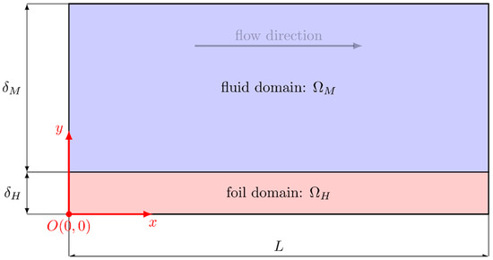
Figure 2.
The scheme of the main domains of the test section (fluid and foil) considered in the calculations.
The heat equation [19] with an internal heat source was used to describe the temperature distribution in the heated wall of the minichannel:
where: TH—the heated wall temperature, ,
- L—the minichannel length, —the heated wall thickness, —Laplacian,—the heated wall thermal diffusivity coefficient, ,
- —the heated wall thermal conductivity, —the heated wall density,
- —the heated wall specific heat,
- —the internal heat source, , q—the heat flux, ,
- A—cross-sectional area of the heated wall, I—the current supplied to the foil, ΔU—the voltage drop across the heated wall.
The Fourier-Kirchhoff equation [19] defines the non-stationary temperature field of the flowing fluid as follows:
where , —the fluid temperature,
- —the minichannel depth, —fluid thermal diffusivity coefficient, ,
- —fluid thermal conductivity, —fluid density, —fluid specific heat, —component of the fluid velocity vector.
The boundary and initial conditions took into consideration measurements of the fluid temperature at the minichannel inlet and outlet as well as the recorded temperature of the heated wall and the assumption of ideal thermal insulation on the respective edges.
where: , —temperatures at inlet and outlet to the minichannel, respectively, and —temperature on the outer side of the heated wall. All data were obtained from experimental measurements.
The heat transfer problem in minichannels was solved by two numerical methods: FEM with Trefftz-type basis functions (FEMT) and ADINA software. The boundary and initial conditions listed above were used to solve the inverse heat transfer problem by FEMT. In the approach proposed by ADINA software, the direct heat transfer problem was solved with the application of additional boundary conditions formulated in Section 3.2.
3.1. FEM with Trefftz-Type Basis Functions (FEMT)
The inverse heat transfer problem described by Equations (1)–(9) was solved, as in [20], by a special calculation procedure based on FEM, combined with Trefftz functions in the domain divided into space-time cuboidal and 8-nodes elements. This calculation method consists of interpolating the unknown temperature function in the nodes of elements, using the time-dependent Trefftz functions, determined for the Fourier-Kirchhoff equation [20] and for the heat equation [21]. When determining the Trefftz functions for the heat equation, the parabolic velocity profile was taken into account as follows:
where —mean fluid velocity obtained based on total mass flow rate (see Table 1) and the density of the fluid.
By minimizing the functional describing the mean square error of the approximate solution at the boundary, at the initial time and along the common edges of adjacent subdomains, unknown values of the temperature function at the nodes were determined [22].
3.2. ADINA Software
The ADINA software, version 9.2, was used to solve the stated problem. In addition to Equations (1) and (2) that express the conservation of energy principle in the fluid and foil domains, respectively, equations that describe the conservation of mass and momentum principles were solved [23]. As a consequence, velocity and pressure p fields in fluid domain are independent variables, and it was not necessary to assume a fixed shape of the x-component of the velocity field as in Equation (10). Instead, additional boundary conditions had to be introduced as follows:
where , , is the absolute pressure at the outlet (known from the experiment—see Table 1).
Equation (11) represents the assumption that there are no heat losses to the environment at the boundary of the minichannel. Equations (12) and (13) represent the standard no-slip condition at the boundaries perpendicular to the flow direction. Equations (14) and (15) set the velocity of the fluid at the inlet and the absolute pressure of the fluid at the outlet, respectively.
The transient type of analysis was applied, and 2D 4-node, planar FCBI elements (flow-condition based interpolation) were used. The mesh used in the simulations was regular: elements were rectangles, and their sides along the length of the minichannel (x direction, Figure 2) have equal lengths in the perpendicular direction (y direction, Figure 2), the lengths of sides gradually decreased with the smallest sides near the fluid-foil interface. The number of subdivisions of lines in the direction perpendicular to the minichannel length (in the fluid and foil domains) were proportional to the number of subdivisions in the direction along the minichannel length. The mesh density depended only on one parameter, the number of subdivisions in the direction along the length of the minichannel (let us denote this number by N). The typical FE mesh used in the calculation in ADINA software is illustrated in Figure 3.
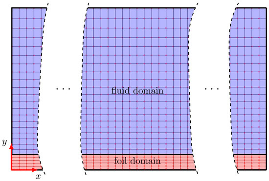
Figure 3.
A typical FE mesh used in the computation in ADINA software.
The unconditionally stable implicit time integration method was used with a time step equal to 1 s.
The mesh density, as essential for the simulations, was taken into special consideration. Various values of the parameter N (i.e., mesh densities) were tested, and the relationship between N and the values of the heat transfer coefficient in time for fixed x was investigated. An N was selected, for which the maximum relative difference between the distributions of the heat transfer coefficients in time and the fixed coordinate x for subsequent values of N was less than 5%. This goal was achieved for N = 500. The resulting mesh contains 18,000 elements (2000 elements in the foil domain and 16,000 in the fluid domain) and 19,038 nodes.
The procedure described above was carried out for the FEM simulation of the experiment at . However, the same FE mesh was also used in other calculations.
4. Results and Discussion
In general, the results are presented as boiling curves and local heat transfer coefficients. Moreover, experimental data, covering the temperature of the heater and the heat flux values, are also visualized.
Figure 4a–k present boiling curves, i.e., dependencies between heat flux (density) and the temperature difference between the heated wall and the bulk fluid temperature, for selected mass flow rates Qm (see Table 1). Each graph illustrates three curves, depending on the location along the minichannel length from which temperatures were taken: x/L = 1/3 (green curve), x/L = 1/2 (blue curve) and x/L = 2/3 (red curve). The data presented in these graphs were taken from experimental measurements for the entire experiment. The black arrows indicate the moments of the experiments taken into consideration in further analyses, with regard in detail to the points referring to subcooled boiling initiation, for curves marked in red. Furthermore, Figure 4l shows the heat flux as a function of time for the entire experiment at Qm = 55 [kg/h]. The red ellipse indicates a part of the experiment while the subcooled boiling starts, which was considered in the FEM simulations. It should be explained that, in calculations, only data from the experiment concerning boiling incipience and subcooled boiling region were considered.
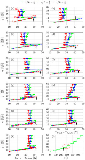
Figure 4.
(a–k) The boiling curves obtained for selected distances from the minichannel inlet: x/L = 1/3 (green curve), x/L = 1/2 (blue curve) and x/L = 2/3 (red curve), corresponding to following mass flow rates: (a) ; (b) ; (c) ; (d) ; (e) ; (f) ; (g) ; (h) ; (i) ; (j) (k) ; (l) heat flux versus time for the whole experiment, ; other data and parameters of the experimental series are listed in Table 1. The red ellipse indicates subcooled boiling region, whereas black arrows indicate onset of boiling (ONB).
During the construction of the boiling curves, the experimental data were plotted as a full line in Figure 4a to show a typical trend to emphasise the continuity of measurement. At the beginning, while increasing the heat flux (from point A to point ONB—onset of boiling), the heat transfer between the heated wall and the fluid proceeds by single phase forced convection. In the foil adjacent area, the liquid becomes superheated, whereas, in the flow core, it remains subcooled. The increase in activation of the vapour nuclei on the heated wall and their spontaneous nucleation cause a temperature drop on the heater surface, resulting from the spontaneous formation of vapour bubbles in the adjacent layer to the heated wall. Bubbles act as internal heat sinks and absorb a significant amount of energy transferred to the liquid. It is visible as a drop from ONB to point C, which is evidence that ‘nucleation hysteresis’ occurred [6]. A further increase in the heat flux supplied to the heater leads to developed nucleate boiling, Section C-D.
When analysing the results presented in Figure 4i–k, it was observed that the temperature difference between the heated wall and the bulk fluid temperature at the ONB point was the lowest compared to all other boiling curves presented. The curves shown in Figure 4i–k relate to the highest value of the mass flow rate. Furthermore, the highest temperature difference was gained for the boiling curve corresponding to , Figure 4e. When comparing the boiling curves with the distance from the inlet, it was observed that the curves generated at x/L = 2/3 were characterized by the lowest temperature difference at the ONB, which was related to the lowest mass flow rate set, Figure 4a–c. Moreover, when the part of the boiling curves that corresponds to saturated boiling (Section C-D) is taken into consideration, it is noticed that line C-D is almost parallelly shifted in the X axis (in such a manner that heat fluxes correspond to lower temperature differences with increasing distance from the inlet). It should also be added that similar courses of part of the boiling curves correspond to a single convection process (Section A-ONB).
The local heat transfer coefficients on the heated wall-fluid contact were calculated from the following formula:
where the temperature distributions at the fluid and foil domains were taken from the results of the numerical calculations (using Trefftz functions or ADINA software). Temperature is a reference temperature, i.e., temperature in the fluid domain at fixed line . This line was selected with the assumption that temperature does not change much in the direction perpendicular to the length of the minichannel and is approximately equal to the temperature at the inlet of the minichannel. It was assumed that , as in [24].
In addition, to verify the results obtained from the numerical methods, the local heat transfer coefficients in the heated wall-fluid contact were also calculated from a simple formula, based only on experimental measurements, as in [20]:
where were defined in Section 3.
Temperature distribution is assumed as follow:
Figure 5 shows the dependence between the heat flux q and the fluid velocity v (corresponding to the mass flow rate Qm). Data from experimental measurements regarding the onset of boiling were taken into consideration.

Figure 5.
Heat flux versus fluid velocity v and mass flow rate Qm, data from all chosen experiments, corresponding to ONB points are marked on boiling curves, indicated by black arrows in Figure 4.
When analysing the relationships shown in Figure 5, with increasing mass flow rate (flow velocity), the heat flux corresponding to the boiling incipience increases. This dependence is particularly recognizable for Qm < 30 [kg/h]. For higher values of Qm, this relationship runs slightly.
The heat transfer coefficient versus the coordinate x along the length of the minichannel is illustrated in Figure 6. The results are based on the data from experiments performed at several values of the mass flow rate. The curves shown in Figure 6a,c present the results of FEM calculations using Trefftz functions, while Figure 6b,d are the results from numerical computation with the aid of ADINA software. It should be explained that the results illustrated in Figure 6 correspond to the selected heat flux, corresponding to the onset of boiling (the point marked ONB, indicated by the black arrows on the boiling curves shown in Figure 4).
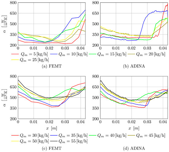
Figure 6.
The heat transfer coefficient versus coordinate x along the length of the minichannel determined using Trefftz functions and with the aid of ADINA software, the results obtained for several values of mass flow rate : (a,b) and (c,d) . The data corresponding to ONB points are indicated by black arrows in Figure 4.
After a comparable analysis of the results presented in Figure 6, similar values and coefficient distributions were obtained from two calculation methods. When analysing the results collected at Qm = 5–25 kg/h, the local heat transfer coefficients determined with the help of the ADINA program turned out to be higher compared to the results of the heat transfer coefficient obtained from FEMT (except the channel outlet region). It should be noted that the results gained at Qm = 10 kg/h differ slightly compared to the results found at other mass flow values. The maximum value of the heat transfer coefficient for this mass flow rate value is reached closer to the minichannel inlet part. Furthermore, when the results are analysed at the channel inlet, it can be indicated that, for lower fluid velocities, lower values of the heat transfer coefficient were obtained, Figure 6a,b. In addition, the heat transfer coefficient increases with distance from the minichannel and is reached to the maximum at the outlet. However, for higher mass flow rates, Figure 6c,d, higher coefficient values were obtained at the inlet compared to those collected at lower mass flow rates. Furthermore, the heat transfer coefficient decreases with increasing distance, at distances up to 3/4 minichannel length (starting from the inlet). The minimum values of the heat transfer coefficient are located near the middle of the minichannel. When the inlet area of the channel is analysed, with increasing fluid velocities, a decrease of the heat transfer coefficient is observed. Furthermore, at the outlet, similar coefficient values were obtained, comparing the results is illustrated in Figure 6a,b and Figure 6c,d.
In order to emphasize the comparison of the distributions of the heat transfer coefficient, the coefficient versus the coordinate x along the length of the minichannel is shown in Figure 7a,c,e. The graphs present the results determined from ADINA software (green curves), with the help of Trefftz functions (blue curves) and additionally according to the 1D mathematical method of calculations (red curves). The distributions of the heat transfer coefficient were captured for three selected mass flow rates , and ). Furthermore, in Figure 7b,d,f, the relative differences between the results of the heat transfer coefficient are highlighted.
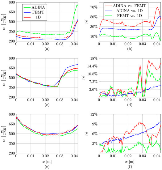
Figure 7.
The comparison of the distributions of the heat transfer coefficient versus coordinate x along the length of the minichannel obtained from three calculation methods (FEM using Trefftz functions, ADINA software and the 1D method) (a,c,e) and relative differences (rd) between the results (b,d,f). The data collected for: (a,b) , (c,d) , (e,f) . The data corresponding to ONB points are indicated by black arrows in Figure 4.
The relative difference between the heat transfer coefficients named α1 and α2 as the results of using two selected calculation methods (considering three methods described above) was estimated from the following formula:
The results presented in Figure 7 confirm the previous comments concerning the exposed dependencies. At lower mass fluxes, the heat transfer coefficient increased in the outlet part of the channel. Furthermore, the minimum values of the coefficient are recognizable in the middle part of the channel for the average mass flow rates. However: (i) at the highest flow rates, the highest heat transfer coefficient is detected at the inlet, (ii) at the medium flow rates, higher values of the transfer coefficient are observed in the middle part of the channel, and (iii) at the highest flow rates, the highest heat transfer coefficient is observed near the inlet and higher in the middle of the channel, compared to small and average . In addition, for low mass flow rates, Figure 7a,b, greater discrepancies (up to 70%) are found when analysing the results compared to the results collected at higher mass flow rates, Figure 7c,d,e, for which differences reached a dozen or so per cent. The lowest values of relative differences are obtained for the highest . Generally, for the lowest and the highest values of , the lowest relative differences rd between the results for FEMT vs. 1D was noted (Figure 7b,f, but for Qm = 30 [kg/h], the trend is not clear (Figure 7d). Furthermore, lower rd values were achieved close to the minichannel inlet.
Figure 8 illustrates the heat transfer coefficient versus fluid velocity/mass flow rate for three selected distances from the minichannel inlet defined as x/L, in detail as follows: x/L = 0.25, 0.5 and 0.75. This figure also refers to the data captured during boiling incipience. The results are obtained by calculations performed with the aid of ADINA software and (Figure 8a) and using Trefftz functions (Figure 8b).
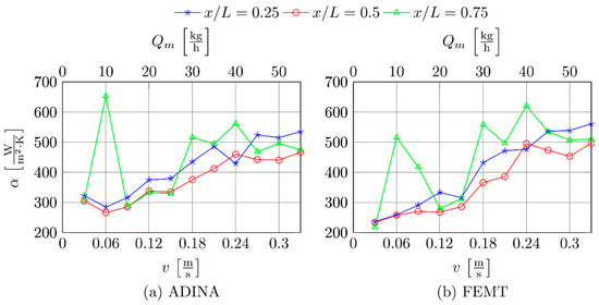
Figure 8.
The heat transfer coefficient versus fluid velocity/mass flow rate for three selected distances from the minichannel inlet was defined as x/l, the results obtained from the calculations: (a) with the help of ADINA software and (b) using Trefftz functions. The data corresponding to ONB points are indicated by black arrows in Figure 4.
Upon analysis of the results shown in Figure 8, it was observed that, in general with increasing mass flow, the heat transfer coefficient increased. However, the results obtained for the distance defined as x/L = 0.5 showed several extremums, while the maximum heat transfer coefficient occurs at . Furthermore, the greatest data scatter was noticed in the dependence constructed for x/L = 0.75. It can be noted that the dependence obtained for x/L = 0.5 corresponds to the lowest values of the heat transfer coefficient.
The distributions of the heater temperature versus the coordinate x along the channel length and time, obtained from the infrared thermography measurement performed on the outer foil surface, for 11 values of mass flow rate, are presented in Figure 9a–k. Furthermore, the fluid temperature on the reference line, as the result of the calculations resulting from the ADINA software (on the basis of data for ) is additionally shown in in Figure 9l. Sharp differences between values are characteristic for lower mass flow rates, Figure 9a–e. For higher flow rates, the recorded data are blurred, Figure 9f–k. Furthermore, changes in fluid temperature are uniform and stable, Figure 9l. It can be added that the lowest temperature of the heated foil near the channel outlet was noticed for , Figure 9b. It resulted in the highest values of the heat transfer coefficient, achieved for in Figure 8. The time intervals considered in FEM simulations relate to the boiling incipience and the subcooled boiling region. In numerical computation, it was assumed that the initial time is zero. In Figure 9k, the numbering of moments of time, related to the whole experiment, was also shown.
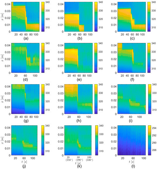
Figure 9.
The distribution of the heater temperature versus coordinate x and time, based on infrared thermography measurement, performed on the outer foil surface, mass flow rate: (a) ; (b) ; (c) ; (d) ; (e) ; (f) ; (g) ; (h) ; (i) ; (j) ; (k) , *—the numbering of moments of time related to the entire experiment (see Figure 4l); (l) the fluid temperature at the reference line (see Figure 2), , calculations according to ADINA software.
Figure 10 shows distributions of the heat transfer coefficient versus coordinate x and time t, obtained using ADINA software, Figure 10a,d,g and Trefftz functions, Figure 10b,e,h, based on data collected for three values of the mass flow rate. Furthermore, the distribution of the relative differences between the heat transfer coefficient, determined according to two calculation methods (ADINA and FEMT) for the selected mass flow rate (), is presented in Figure 10h.
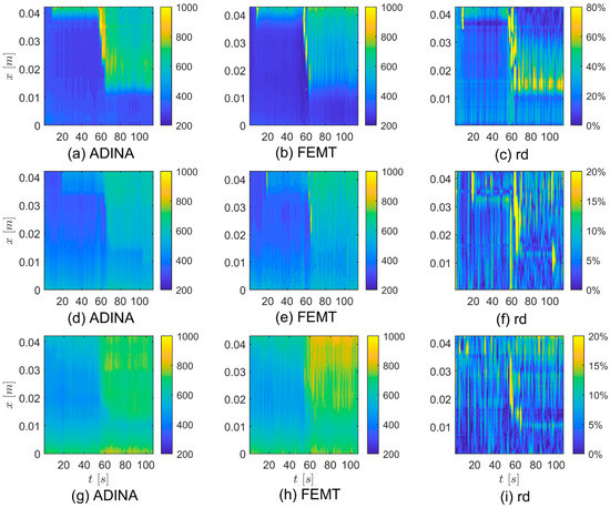
Figure 10.
The distribution of the heat transfer coefficient versus coordinate x and time t obtained using ADINA software (a,d,g) and FEMT with applying Trefftz functions (b,e,f); the relative differences between local heat transfer coefficients as the results of calculations according to these two methods (ADINA and FEMT). The calculations performed on the basis of the results of experiments were performed at three values of mass flow rate: (a–c) ; (d–f) ; (g–i) .
When analysing the dependence of the heat transfer coefficient versus coordinate x and time presented in Figure 10, it can be seen that after about 60 s there was a sudden increase in heat flux (see Figure 4l), which corresponds to a stepwise increase in the heat transfer coefficient. Generally, similar distributions of the local heat transfer coefficient were achieved. Furthermore, there is good agreement between the heat transfer coefficients, determined with the help of ADINA software, and based on the FEMT calculation using Trefftz functions, Figure 10c,f,i. It can also be noticed that a high level of relative differences is reached between the results of the numerical calculations in small regions of the t and x variation domain, but in the rest of this domain, the relative differences are low. Therefore, even though there is a high maximum of relative differences, their average values appeared to be low. For the lowest mass flow rate, significantly higher relative differences were achieved up to 80%, Figure 10c, compared to the results obtained for higher mass flow rates, Figure 10f,i. It can be emphasized that, during experiments, the heat flux increases over time (the experimental methodology is described in Section ‘Experimental background’), while the example dependence of the heat flux, as a function of time for the entire experiment, is given in Figure 4l, for . It can be observed that maximum relative differences between heat transfer coefficients, according to both calculation methods, occur when there is a sharp increase in the heat flux.
In Figure 11 are shown the average values of relative differences of the heat transfer coefficient, obtained from calculations performed using different calculation methods (ADINA software, FEMT using Trefftz functions and the 1D approach), as a function of the mass flow rate.

Figure 11.
The average values of relative differences of the heat transfer coefficient obtained using different approaches: ADINA software, FEMT and 1D approach versus flow rate .
When analysing the graph, it can be found that, with an increase in mass flow rate, the mean relative differences decrease. It should be underlined that for > the relative differences are below 10%. The highest relative differences occurred for the lowest mass flow rate, especially and when FEMT versus 1D method or ADINA versus FEMT were considered (value of relative differences greater than 40%). It can be mentioned that, considering the resulting relative differences between ADINA versus FEMT, the adoption of the reference line is an essential issue. In the future, the authors plan to investigate the influence of assuming the reference line in calculations, considering the thickness of the hydraulic and thermal boundary layers.
5. Conclusions
This article describes an investigation of subcooled boiling during FC-72 flow in a heat sink with a group of five parallel minichannels heated asymmetrically. The focus of the authors was the heat transfer characteristics at boiling incipience and the subcooled flow boiling region. The results of time-dependent experiments were the basis for mathematical calculations. Infrared thermography helped to measure the temperature on the heater surface, while other flow and thermal parameters were recorded by specialized measuring devices. In order to solve the heat transfer problem, two numerical methods, based on the FEM, were used. One was based on the Trefftz functions (FEMT), and the ADINA program was the other. Using FEMT, the inverse heat transfer problem was solved, while due to the ADINA program, a solution to a direct heat transfer problem was obtained. In an experimental way, the effect of the mass flow rate on the heat transfer coefficients was investigated. The results achieved with two calculation methods were discussed with special attention to the distributions of the temperature and heat transfer coefficient, considering the relation to the fluid mass flow rate.
The boiling curves and heat transfer coefficient distributions were presented. Furthermore, the distribution of the temperature of the heater and the heat flux are shown. It was found that, with an increase in mass flow rate, the heat flux corresponding to the boiling incipience increases. This dependence was particularly recognizable for Qm < 30 [kg/h].
After a comparable analysis of the results obtained, it was seen that similar values and coefficient distributions were obtained from two calculation methods (FEMT and ADINA software). Furthermore, in general, as the mass flow increased, the heat transfer coefficient increased. When the results at the channel inlet were analysed, it was indicated that, for lower fluid velocities, lower values of the heat transfer coefficient were obtained. In addition, the heat transfer coefficient increases with the distance from the minichannel. For higher mass flow rates, higher coefficient values were obtained at the inlet compared to those collected at a lower mass flow rate. The minimum values of the heat transfer coefficient were located near the middle of the minichannel. In the inlet area of the channel, a decrease of the heat transfer coefficient was observed with increasing fluid velocities. Good agreement was found between the heat transfer coefficients determined with the help of the ADINA software and those based on the FEMT calculation. The distribution of the relative differences between the heat transfer coefficient, calculated according to two calculation methods and the 1D calculation method, were determined, visualised and analysed. It was found that above Qm > 15 [kg/h], the average relative differences decrease with increasing mass flow rate. The greatest relative differences occurred when FEMT was compared with other methods at Qm = 10 [kg/h].
The continuation of experimental and theoretical investigations, testing the application of other numerical programs (Ansys Fluent/CFX, Simcenter STAR-CCM+, OpenFOAM) and semi-analytical-numerical methods with application of the Trefftz function in the issue of flow boiling heat transfer in minichannels, are planned by the authors.
Author Contributions
Conceptualization, M.P., B.M. and P.Ł.; data curation, M.P., B.M. and P.Ł.; formal analysis, M.P., B.M. and P.Ł.; funding acquisition, M.P.; investigation, M.P.; methodology, M.P., B.M. and P.Ł.; project administration, M.P.; software, B.M. and P.Ł.; validation, M.P., B.M. and P.Ł.; visualization, P.Ł.; writing—original draft, M.P., B.M. and P.Ł.; writing—review and editing, M.P., B.M. and P.Ł. All authors have read and agreed to the published version of the manuscript.
Funding
This research was funded by the National Science Centre, Poland, grant number UMO-2018/31/B/ST8/01199.
Institutional Review Board Statement
Not applicable.
Informed Consent Statement
Not applicable.
Data Availability Statement
Not applicable.
Conflicts of Interest
The authors declare no conflict of interest.
References
- Kandlikar, S.G.; Grande, W.J. Evolution of Microchannel Flow Passages-Thermohydraulic Performance and Fabrication Technology. Heat Transf. Eng. 2003, 24, 3–17. [Google Scholar] [CrossRef]
- Van den Bergh, W.J.; Moran, H.R.; Dirker, J.; Markides, C.N.; Meyer, J.P. Effect of Low Heat and Mass Fluxes on the Boiling Heat Transfer Coefficient of R-245fa. Int. J. Heat Mass Transf. 2021, 180, 121743. [Google Scholar] [CrossRef]
- Marzoa, M.G.; Ribatski, G.; Thome, J.R. Experimental Flow Boiling Heat Transfer in a Small Polyimide Channel. Appl. Therm. Eng. 2016, 103, 1324–1338. [Google Scholar] [CrossRef]
- Maciejewska, B.; Hozejowska, S.; Piasecka, M. Trefftz-Type Functions Applied for Subcooled Flow Boiling Heat Transfer Calculations in a Minichannel of Different Spatial Orientation. Heat Transf. Eng. 2022. [Google Scholar] [CrossRef]
- Piasecka, M.; Hozejowska, S.; Maciejewska, B.; Pawinska, A. Time-Dependent Heat Transfer Calculations with Trefftz and Picard Methods for Flow Boiling in a Mini-Channel Heat Sink. Energies 2021, 14, 1832. [Google Scholar] [CrossRef]
- Piasecka, M.; Strąk, K.; Maciejewska, B. Heat Transfer Characteristics during Flow along Horizontal and Vertical Minichannels. Int. J. Multiph. Flow 2021, 137, 103559. [Google Scholar] [CrossRef]
- Marcinkowski, M.; Taler, D.; Taler, J.; Węglarz, K. Comparison of Individual Air-Side Row-By-Row Heat Transfer Coefficient Correlations on Four-Row Finned-Tube Heat Exchangers. Heat Transf. Eng. 2022, 1–13. [Google Scholar] [CrossRef]
- Che, M.; Elbel, S. Comparison of Local and Averaged Air-Side Heat Transfer Coefficients on Fin-and-Tube Heat Exchangers Obtained With Experimental and Numerical Methods. J. Therm. Sci. Eng. Appl. 2022, 14, 071013. [Google Scholar] [CrossRef]
- Memon, A.A.; Anwaar, H.; Muhammad, T.; Alharbi, A.A.; Alshomrani, A.S.; Aladwani, Y.R. A Forced Convection of Water-Aluminum Oxide Nanofluids in a Square Cavity Containing a Circular Rotating Disk of Unit Speed with High Reynolds Number: A Comsol Multiphysics Study. Case Stud. Therm. Eng. 2022, 39, 102370. [Google Scholar] [CrossRef]
- Li, Z.; Pan, J.; Peng, H.; Chen, D.; Lu, W.; Wu, H. Numerical Study on Subcooled Flow Boiling in Narrow Rectangular Channel Based on OpenFOAM. Prog. Nucl. Energy 2022, 154, 104451. [Google Scholar] [CrossRef]
- Georgoulas, A.; Andredaki, M.; Marengo, M. An Enhanced VOF Method Coupled with Heat Transfer and Phase Change to Characterise Bubble Detachment in Saturated Pool Boiling. Energies 2017, 10, 272. [Google Scholar] [CrossRef]
- Piasecka, M.; Piasecki, A.; Dadas, N. Experimental Study and CFD Modeling of Fluid Flow and Heat Transfer Characteristics in a Mini-Channel Heat Sink Using Simcenter STAR-CCM+ Software. Energies 2022, 15, 536. [Google Scholar] [CrossRef]
- Peng, Y.; Zarringhalam, M.; Hajian, M.; Toghraie, D.; Tadi, S.J.; Afrand, M. Empowering the Boiling Condition of Argon Flow inside a Rectangular Microchannel with Suspending Silver Nanoparticles by Using of Molecular Dynamics Simulation. J. Mol. Liq. 2019, 295, 111721. [Google Scholar] [CrossRef]
- Zarringhalam, M.; Ahmadi-Danesh-Ashtiani, M.; Toghraie, D.; Fazaeli, R. Molecular Dynamic Simulation to Study the Effects of Roughness Elements with Cone Geometry on the Boiling Flow inside a Microchannel. Int. J. Heat Mass Transf. 2019, 141, 1–8. [Google Scholar] [CrossRef]
- Zhang, H.; Bathe, K.J. Direct and Iterative Computing of Fluid Flows Fully Coupled with Structures. In Proceedings of the First MIT Conference on Computational Fluid and Solid Mechanics, Cambridge, MA, USA, 12–15 June 2001; Elsevier Science: Oxford, UK, 2001. [Google Scholar]
- Khimenko, A.V.; Tikhomirov, D.A.; Vasilyev, A.N.; Samarin, G.N.; Shepovalova, O.V. Numerical Simulation of the Thermal State and Selecting the Shape of Air Channels in Heat-Storage Cells of Electric-Thermal Storage. Energy Rep. 2022, 8, 1450–1463. [Google Scholar] [CrossRef]
- Wu, W.; Guo, T.; Peng, C.; Li, X.; Li, X.; Zhang, Z.; He, Z. FSI Simulation of the Suction Valve on the Piston for Reciprocating Compressors. Int. J. Refrig. 2022, 137, 14–21. [Google Scholar] [CrossRef]
- Piasecka, M.; Strąk, K. Characteristics of Refrigerant Boiling Heat Transfer in Rectangular Mini-Channels during Various Flow Orientations. Energies 2021, 14, 4891. [Google Scholar] [CrossRef]
- Poniewski, M.E.; Hożejowska, S.; Kaniowski, R.; Maciejewska, B.; Pastuszko, R.; Piasecka, M.; Wójcik, T.M. Encyclopedia of Two-Phase Heat Transfer and Flow I: Fundamentals and Methods Volume 4: Special Topics in Pool and Flow Boiling; Thome, J.R., Ed.; World Scientific: Singapore, 2015; ISBN 978-981-4623-20-9. [Google Scholar]
- Maciejewska, B.; Piasecka, M. Time-Dependent Study of Boiling Heat Transfer Coefficient in a Vertical Minichannel. Int. J. Numer. Methods Heat Fluid Flow 2019, 30, 2953–2969. [Google Scholar] [CrossRef]
- Cialkowski, M.; Grysa, K. Trefftz Method in Solving the Inverse Problems. J. Inverse Ill-Posed Probl. 2010, 18, 595–616. [Google Scholar] [CrossRef]
- Maciejewska, B.; Piasecka, M. Trefftz Function-Based Thermal Solution of Inverse Problem in Unsteady-State Flow Boiling Heat Transfer in a Minichannel. Int. J. Heat Mass Transf. 2017, 107, 925–933. [Google Scholar] [CrossRef]
- ADINA R&D Inc. ADINA Theory and Modeling Guide, Volume III: ADINA CFD & FSI; ADINA R&D, Inc.: Watertown, MA, USA, 2015. [Google Scholar]
- Piasecka, M.; Maciejewska, B.; Łabędzki, P. Heat Transfer Coefficient Determination during FC-72 Flow in a Minichannel Heat Sink Using the Trefftz Functions and ADINA Software. Energies 2020, 13, 6647. [Google Scholar] [CrossRef]


Publisher’s Note: MDPI stays neutral with regard to jurisdictional claims in published maps and institutional affiliations. |
© 2022 by the authors. Licensee MDPI, Basel, Switzerland. This article is an open access article distributed under the terms and conditions of the Creative Commons Attribution (CC BY) license (https://creativecommons.org/licenses/by/4.0/).