Using Statistical Shape Models to Optimize TKA Implant Design

Featured Application

This article provides some examples on how Statistical Shape Models can best be used in daily practice of TKA implant design.

Abstract

(1) TKA implants should well fit on each patient’s anatomy. Statistical Shape Models (SSM) statistically represent the anatomy of a given population. The aims of this study were to assess how to generate a valid SSM for implant design and provide guidelines and examples on how to use the SSMs to evaluate the anatomic fit of TKA components. (2) Methods: A Caucasian SSM was built from 120 anatomies (65 female, 55 male) and an Asian SSM was based on 112 patients (75 female, 37 male). These SSMs were used to generate a database of 20 bone models. The AP/ML dimensions of the bone models were compared to those of the input population. Design input parameters, such as the tibial contour, trochlea, and femur curvature were extracted from the SSMs. Femur and patella components were virtually implanted on the bone models. (3) Results: the dimensions of the generated bone models well represented the population. The overhang of the femoral component as well as the coverage and peak restoration of the patella component were visualized. (4) Conclusions: SSMs can be used to efficiently gain input into TKA design and evaluate the implant fit on the studied population.

1. Introduction

To restore good function of the knee joint, total knee arthroplasty (TKA) implants should fit well to each patient’s anatomy. On the femoral side, a good fit of the component is crucial to obtain good kinematics and a stable knee joint. Overhang of the component can cause soft-tissue irritation [1,2], while overstuffing of the patella can lead to anterior knee pain [3]. A good fit between the anterior shield and the trochlea is vital to restore satisfying patellofemoral kinematics [4]. On the tibial side, sufficient bone coverage is important [5] while overhang should be avoided to prevent soft-tissue irritations [1,6].

Several studies have outlined that implant designs do not fit well to some populations [7,8,9]. Finding a design that fits each patient well is indeed very challenging, as bone morphology greatly varies among patients. Besides ethnicity, other factors, such as gender and pathology, also influence the bone morphology.

Before introducing a new implant to the market, implant manufacturers need to prove that the design fits well to the patient’s anatomy. The norm for joint replacement implants ISO 21534 requires ‘the suitability of the dimensions and shape of the implant for the population for which it is intended’ be ensured. However, there is currently no clear guideline on how to best proceed.

Currently the fit of implants is mainly assessed in the three following ways:

Prototype or trial implants are placed intraoperatively on patients’ bones [2,10]. The main limitation is the restricted number of available bones. Additionally, the number of implant sizes that can be tested, the number of dimensions that can be measured intra-operatively, and the accuracy with which those measurements can be performed are limited.

The most common method is the use of 2D or 3D medical images (radiographs, CT or MRI data) to collect specific dimensions on a specific population. For example several studies report the anteroposterior (AP) and mediolateral (ML) dimensions of the distal femur and proximal tibia obtained from medical images [7,8,9,11,12,13,14,15]. These dimensions can then be compared to the implants’ dimensions. This provides the first valuable information on the needed dimensions in an implant portfolio. However, it is limited to a few dimensions in specific areas of the implant. Moreover, it must be carefully considered whether the definition of the dimensions corresponds exactly to the analyzed implant dimension. For example, the location at which the AP dimension of the proximal tibia is measured to serve as a reference for the AP dimension of the tibial plate has to be considered with great care.

Finally, 3D bone models generated from medical images can be used in different ways to evaluate the implant fit:

A ‘virtual implantation’ enables the placement of implant components on 3D bone models. The fit can then be assessed by performing different measurements, such as overhang and underhang of the components. The challenge is to place the components in a clinically realistic way. In studies including a high volume of datasets, algorithms were developed to enable an automated placement of the components [16]. However, these algorithms cannot take individual specificities into account, which would influence the component placement during surgery. Furthermore, the quality of the virtual implantation is limited due to the lack of information on the soft tissue situation.

Three-dimensional bone models can also be used to extract information about the 3D shape of relevant surfaces, such as the shape of the tibial plateau. For example Dai [17] provides a statistical description of the proximal tibia plateau, which can then be used to define the optimal contour of a tibial component.

Finally, 3D bone models can be used to generate Statistical Shape Models (SSM) [18]. These models are created from many—typically over 100—bone models reconstructed from CT or MRI data of a given population. The SSM is built by aligning all bone models, computing an average geometry, and performing a principal component analysis on the deviations between the individual models and the average geometry. The resulting principal components are called modes of (geometric) variation. In a decreasing order of importance, these modes show the most important changes in geometry witnessed in the studied population. Modes can then be tuned to generate different sizes and geometries. The SSM thus corresponds to a statistical representation of the anatomy of the input population. Hence, it is a powerful tool to reduce the number of bone models to be analyzed in order to obtain statistically relevant measurements.

Once the SSM is built, the question arises of how to best use it to validate that the size and shape of TKA components are well adapted to each patient’s anatomy. To the authors’ knowledge, there is no literature describing how to use SSMs to evaluate the anatomical fit of TKA implant design. The aims of this study were (1) to evaluate how to generate a valid SSM for implant design and (2) provide examples on how to use the SSMs to evaluate the anatomic fit of TKA components.

2. Materials and Methods

2.1. Generation of the SSM

2.1.1. Selection of Input Data

Beside the methodology used to create the SSM, two main factors influence the quality of a SSM: the number of datasets used and the homogeneity of the studied population. It is therefore important to balance those two factors when selecting the pool of data used to build a model: the more homogeneous the group, the better the model will represent it. The more morphologies are included in the model, the better it will represent a large portion of the population. Therefore, for each application, the input population must be defined with care. When building a SSM to evaluate the fit of TKA implants, it has to be considered whether the input population should be limited to osteoarthritic (OA) patients, or if the model would benefit from including healthy patients as well. Consideration should also be given to whether different SSMs should be generated for each gender and ethnicity, or whether a global model will suffice.

• Impact of pathology: arthritic versus healthy population.

In a preliminary study, the following three SSMs were built: The ‘OA-SSM’ was built from CT scans of 40 arthritic patients (24 female, 16 male, mean age: 68 ± 10 years; range 46–91 years). Patients with Kellgren–Lawrence grades one to three [19] were included. Severe deformities were excluded. The ‘healthy SSM’ was built from CT scans of 40 patients (20 female, 20 male, mean age: 65 ± 14 years, range 29–87 years) with no known knee disorder. The ‘combined SSM’ was built from all the healthy and OA CT scans described above (80 patients, 44 female, 36 male, mean age: 67 ± 12 years, range 29–91 years). The CT scans were obtained from different hospitals across Europe.

The average models of the cortical femur, cortical tibia, and cortical patella of each population (OA, healthy and combined) were compared using two methods. First, the SSMs of the OA and healthy population were aligned to each other by minimizing the root mean square (RMS) error between the two models. This RMS error along with the maximum deviations between the SSMs were used to compare both SSMs. This analysis was performed for all three bones (femur, tibia, patella) via a numerical color map that showed the RMS error between the mesh points of each model (Materialise^® Mimics Innovation Suite Software). Second, to gain insight into how differently the OA and healthy populations behave when they are part of the combined population, Student’s T-test was performed on the mode coefficients of the combined SSM: If the OA and healthy populations were similar, the mode coefficients of the combined SSM would not be statistically different from the mode coefficients of the healthy and OA SSMs.

• Impact of gender and ethnicity.

The impact of mixing genders and ethnicities in different models was evaluated as follows: 92 CT scans from healthy Caucasian and Asian male and female patients were used. One SSM was generated out of the 92 datasets. The CT scans were divided in four equal subgroups according to the ethnicity and gender of the patients (23 CT scans for each group): Caucasian male, Asian male, Asian female, and Caucasian female. One SSM was built for each subgroup, resulting in 4 distinct SSMs. The first mode of variation was used to define different sizes of the model: 5th, 50th and 95th percentile. Each SSM was used to rebuild the anatomy of another subgroup.

Based on these preliminary studies, a Caucasian SSM was built from 120 anatomies (65 female, 55 male) and an Asian one was built from 112 patients (75 female, 37 male).

2.1.2. Generation of the SSM: Choice of the Reference System

The first step in building an SSM is to align all the individual bone models. All bone models need to be represented in a reference system that ensures a good relative alignment of the models. The choice of the reference system influences the robustness of the SSM and its ease of use. The reference system should be easy to identify on all bone models (highly reproducible) and ideally correspond to the landmarks used in clinical practice.

For the tibia, the origin was defined by the mid-point between the most proximal point on the medial tibial spine and the most proximal point on the lateral tibial spine. The proximodistal axis connects the origin to the mid of the malleoli. The AP axis connects the center of posterior cruciate ligament attachment to the medial third of the tibial tuberosity [20].

For the femur, the center of the femoral head and the surgical trans-epicondylar line were used to build the reference system [21,22,23].

For the patella, a coordinate system was defined with one axis aligned with the ridge of the patella [24]. An iterative method was used to define the ridge (proximodistal axis) and the most medial and lateral points of the patella (ML axis). The origin was defined on the usual resection plane of the patella, 6 mm below the patella peak along the AP axis. Use of this coordinate system facilitated resection surface analysis, component placement, and peak medialization analysis. The ability of this reference system to properly align the individual bone models (step 1 in creating the SSM) was evaluated as follows: two alternative SSM were built using the same CT dataset, but using a different method to align the individual bone models. For SSM1, the bone models were aligned by minimizing the RMS error for all models. For SSM2, the individual bone models were aligned using a reference system based on inertial moments. As a result, the SSM built with the patella coordinate system described above enabled us to capture the geometric variance in fewer SSM modes. Thus, the modes were more compact as they captured geometrical trends better.

2.2. Validation of the SSM

Once the SSM was built, a series of tests allowed to ensure that it statistically represents the population well. As the use of SSMs in medical applications is limited, most of these specific validation tests were developed by Materialise^®, Leuven, Belgium. Some preliminary tests are briefly summarized below:

• The Vectorization Errors Test quantifies the error introduced by preprocessing each patient’s bone before it can be used for a SSM (all bones included in the SSM must have the same mesh).
• The Normality Test analyzes whether the population is normally distributed.
• The Compactness Test analyzes how well the modes of variation of the SSM capture the geometrical variation. If the SSM is very compact, the SSM can describe the geometrical variation observed in the input population in a few virtual modes.

Since the focus of this paper is on the use of SSMs for TKA design, the following two tests are described in more detail.

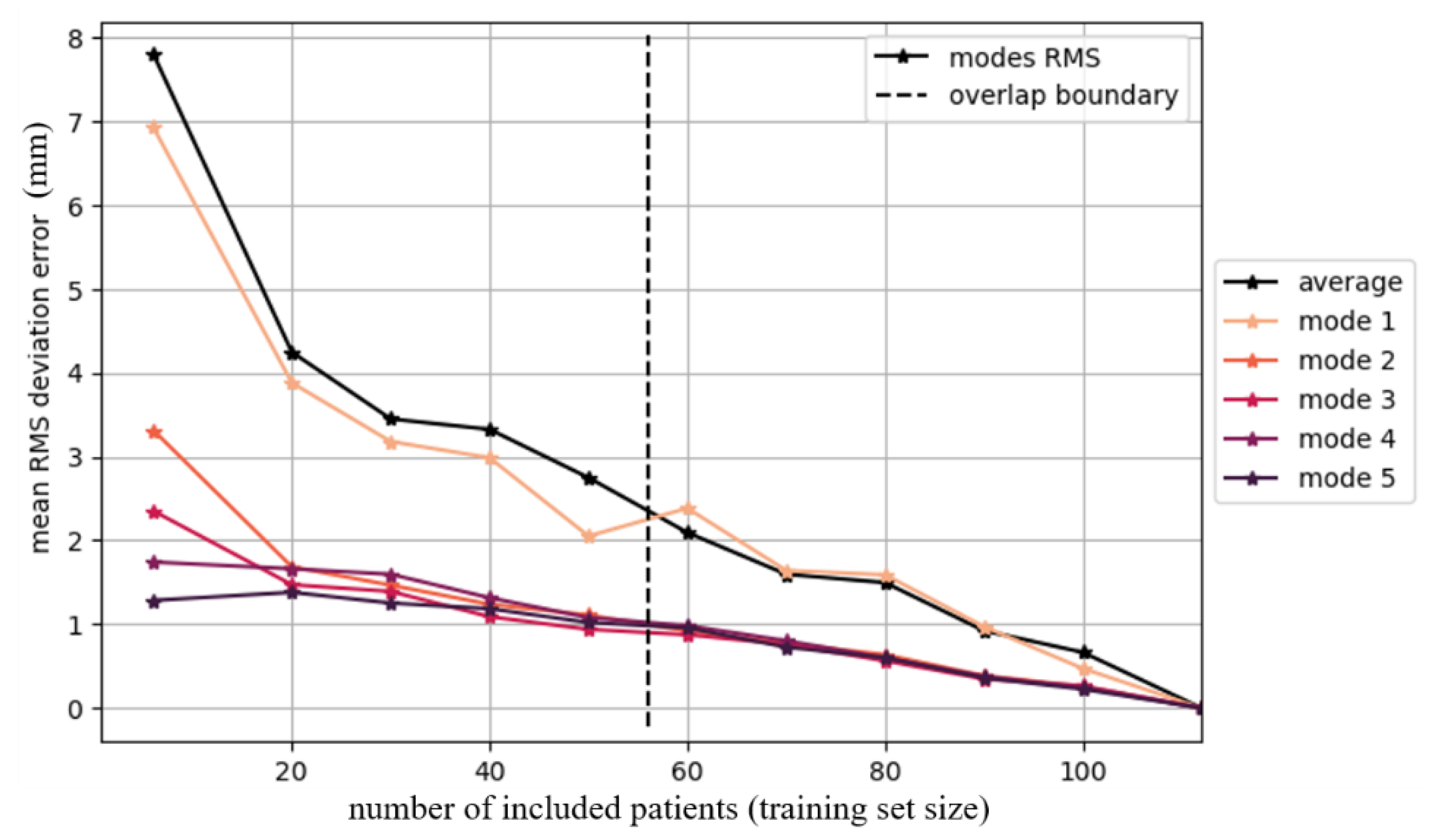
• The Convergence Test analyzes the impact of adding additional patients. If convergence is achieved, additional scans no longer have an impact on the SSM. If convergence is not achieved, this test can be used to calculate the impact of adding new scans to enable the SSM to better capture the input population.

To perform this test, the input data are used to build two independent SSMs. For example, with a population of 100 patients, 50 patients are used to build one SSM; the remaining 50 patients are used to build a second SSM. The RMS error between these SSMs is computed. An increasing amount of datasets is used to compute both SSMs. At a certain point, the populations begin to overlap. For example, with an input population of 100 patients, if 70 patients are used to build the SSMs, 20 patients are used in both models (overlap of 20). The optimal training size is reached when the RMS error reaches the value zero before the populations begin to overlap. This would mean that two models built with independent populations are similar.

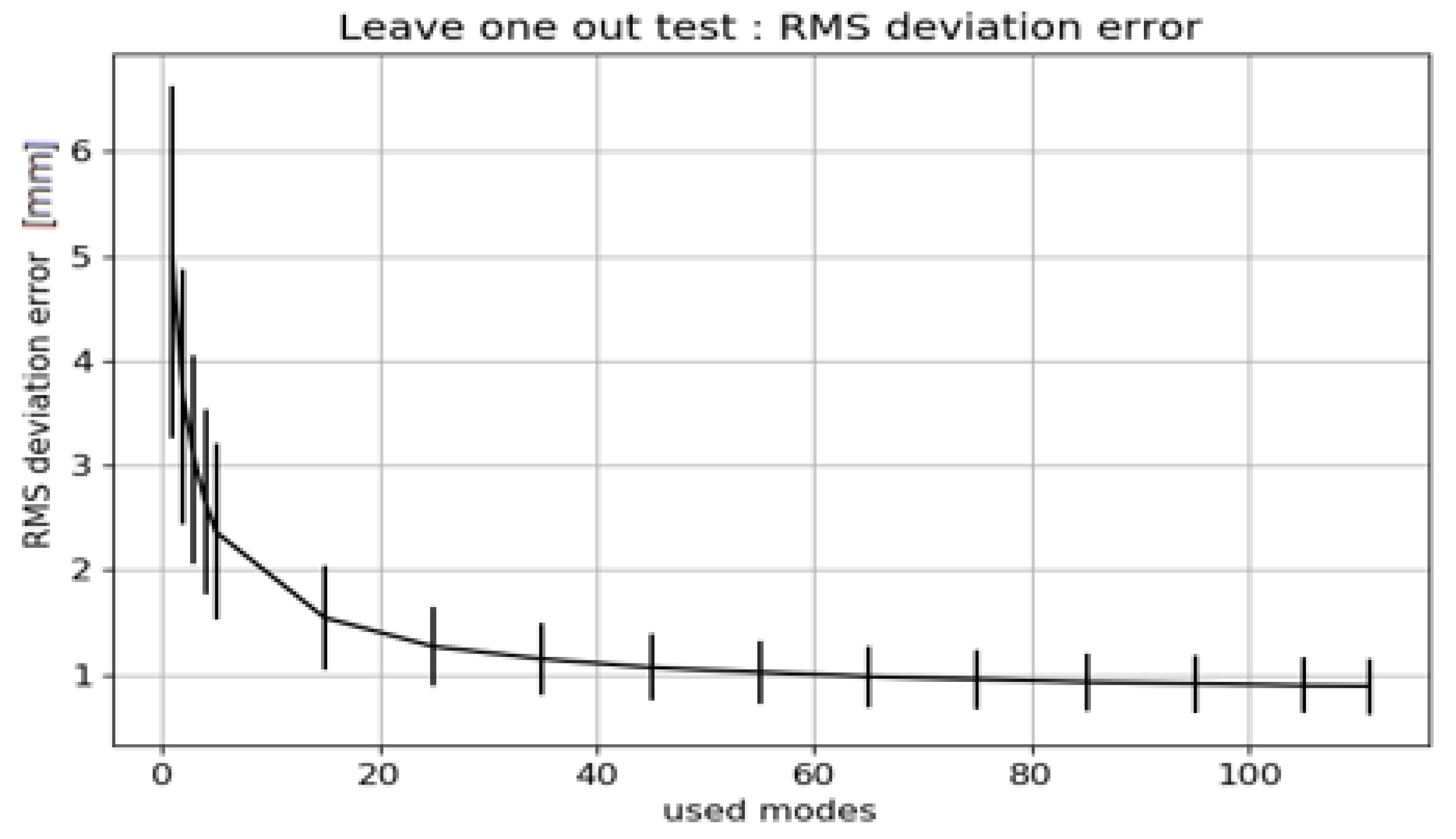
• The Leave-one-out Test analyzes how well the SSM describes patients who are not part of the input population. To perform this test multiple SSMs are generated, leaving out each input patient in turn. For example, with an input population of 112 patients, 112 different SSMs are built with 111 patients. Each of those 111 SSMs is built with an increasing number of modes. The average RMS deviation between the SSMs is computed.

2.3. Use of the SSM

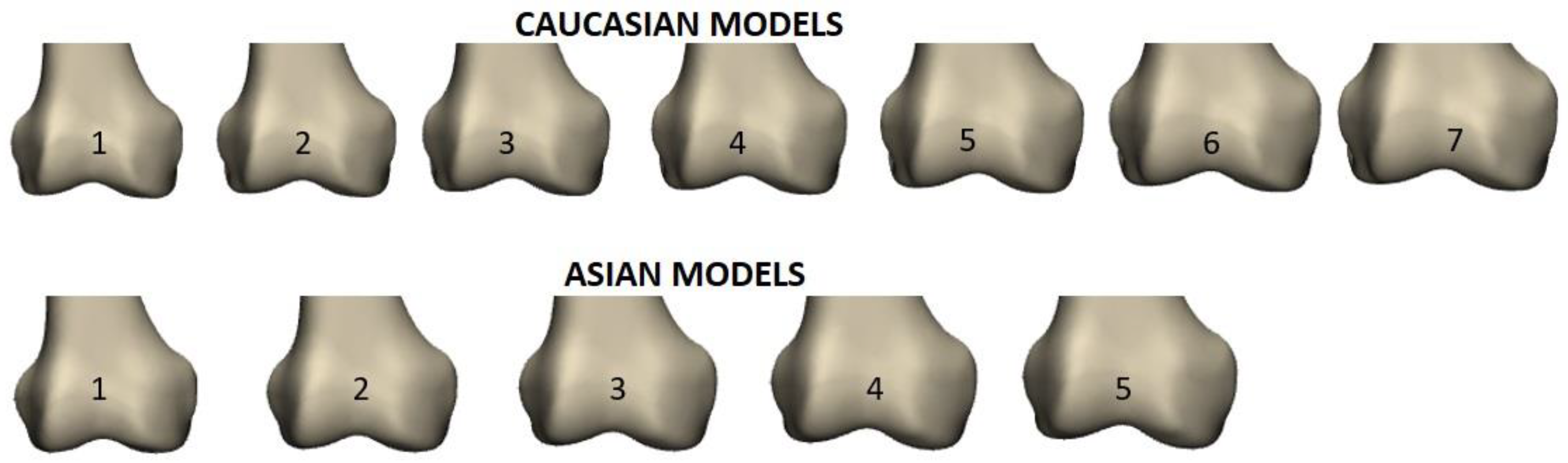
2.3.1. Definition of a Representative Database of 3D Bone Models

The first bone model obtained from the SSM is the geometrical average of the input population. This is considered to be a medium sized model. Since the bone models used for design input and validation must represent anatomies of different shapes and sizes, the first step is to define a database of bone models, that is representative of the population. Seven sizes were defined by tuning the first mode of variation of the Caucasian SSM (Figure 1).

Similarly, 5 sizes were defined using the Asian model. Since the range of AP/ML is smaller in this population, fewer sizes were defined (Figure 1).

To validate this approach, the AP/ML dimensions of the SSMs were compared with the AP/ML dimensions of the individual anatomies. The AP dimensions were defined as the dimensions between the resected cortex and the posterior condyles [25]. The ML dimension was defined as follows: A distal resection was performed orthogonal to the mechanical axis, 9 mm from the most distal point of the condyles. The ML distance along the anatomical trans-epicondylar line was measured.

Ten additional bone models were computed to cover non-average anatomies (patients closer to the borderline of the populations’ dimensions). Ten AP/ML dimensions that well represent the boundary of the population were defined. For each of those AP/ML dimensions, the most average shape of a bone was computed as follows: A large amount of virtual bone models of various sizes and shapes was created using the Markov chain Monte Carlo sample. For each selected AP/ML combination, the virtual bone models with AP/ML dimensions within a certain tolerance of the target dimensions were selected. Within these selected virtual bone models, the most average shape was defined according to the chi-squared distribution. The shape for which the sum of squares of the mode coefficients (which were already normalized by their standard deviation) was closest to zero was defined as the most average. The sum of the squares of the coefficients correspond to the p-value.

2.3.2. Use of SSMs for Design Input

SSMs were used as follows to obtain information for design input. To define the best possible contour for a tibial implant, the averaged sized Caucasian tibia SSM was cut orthogonal to the mechanical axis at different heights (8, 10, and 12 mm). To determine the optimal trochlea design, the depth and path of the native trochlea (deepest points of the trochlea groove) were extracted from different statistical shape model sizes. The resulting splines were projected on the sagittal plane. To evaluate femoral curvature, a spline at the center of the femoral canal was computed for different femur sizes.

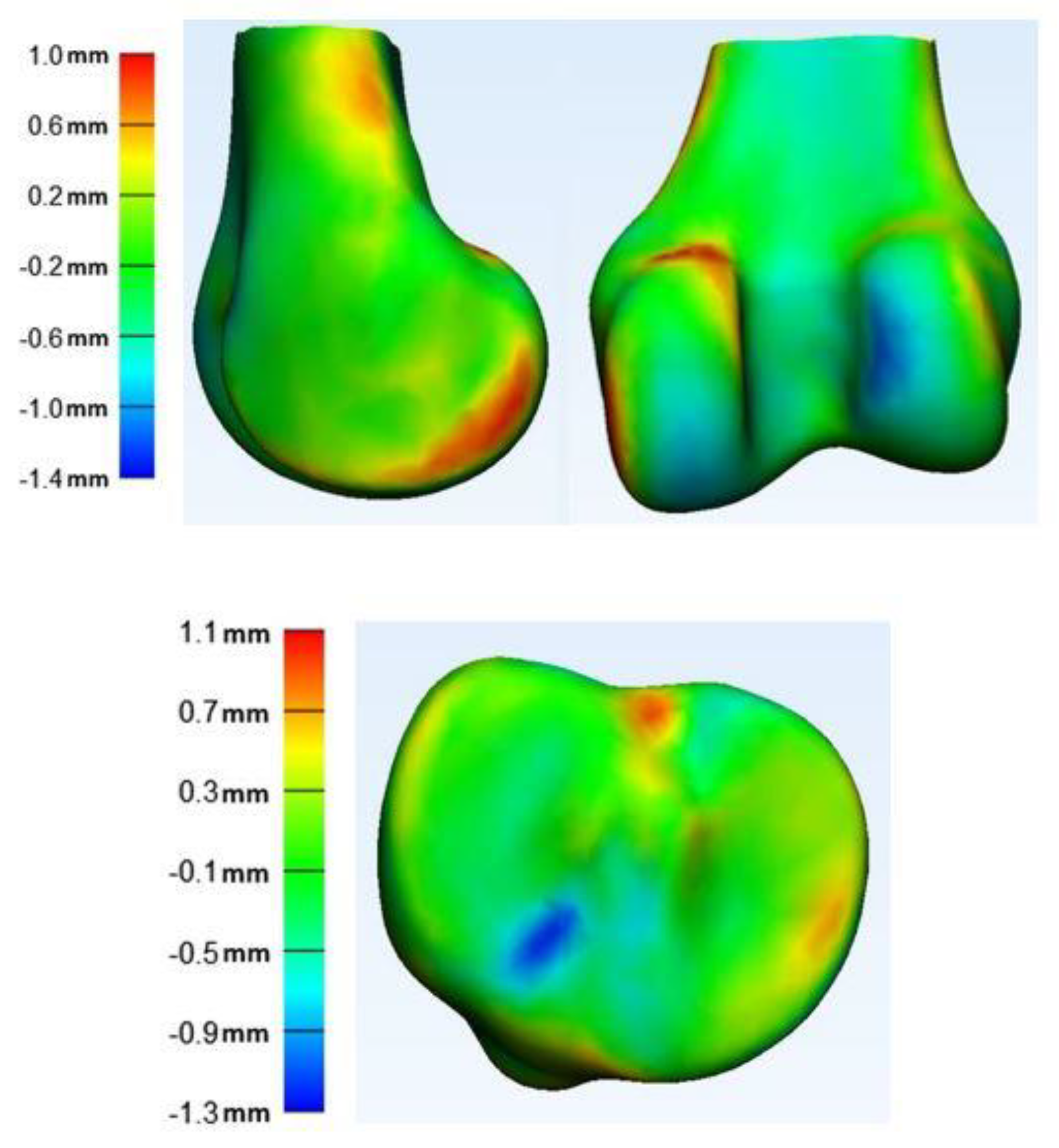
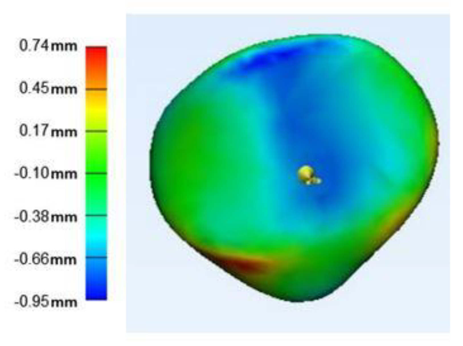
2.3.3. Use of SSMs for Design Validation

SSMs were used as follows to validate implant designs. For the patella, the SSM was cut at 6 mm in its frontal plane. The 3D model of a patella implant (B.Braun Aesculap, Tuttlingen, Germany) was placed on an average-sized SSM. The bony coverage was computed as the percentage of the resected surface covered by the implant. The difference in ML position between the implant peak and the bone peak was measured.

The 3D model of a femoral component (Vega^®, Aesculap, Tuttlingen, Germany) was implanted on seven sizes of the Caucasian and five sizes of the Asian SSM. The overhang and underhang of the component relative to the bone were computed for each of the SSM sizes. A color map was generated to indicate the areas of greatest overhang and underhang.

3. Results

3.1. Generation of the SSM

3.1.1. Selection of Input Data, Impact of Pathology

The numerical color map enabled to visualize the differences between the models (Figure 2). ‘OA-SSM’ and ‘healthy SMM’ differed on average by 1 mm. Some differences were visible on the distal and posterior condyles, as well as on the shape of the articular surface of the patella.

The t-test performed on the combined SSM showed significant differences (p < 0.05) for 3 modes for the femur (mode 4, 10 and 15), 5 modes for the tibia (mode 3, 9, 10, 12 and 19) and 3 modes for the patella (mode 6, 17 and 63).

This pilot study led to the conclusion that the SSM used to represent the arthritic population should preferably be created exclusively from CT scans of arthritic patients if the number of available datasets is sufficient.

3.1.2. Selection of Input Data, Impact of Gender and Ethnicity

The global SSM was able to rebuild the subgroups models with a maximum error of 4.4 mm to 6.5 mm. The subgroup SSMs only managed to recreate the other subgroup’s anatomy with an error between 9.4 and 15.7 mm. Comparing the global SSM with the subgroup SSMs allowed to draw conclusions about the main differences between the anatomies of each subgroups: the Caucasian SSMs were broad in ML, the male Asian SSM were large in AP, and the intercondylar notch of the female Asian SSM proved to be narrow. It was concluded that gender and ethnicity have an important influence on the SSM and thus are distinguishable features in the populations.

3.2. Generation of the SSM: Validation

• For the SSMs used in this study 99% of the Vectorization Errors were less than 0.5 mm and the assumption of normally distributed populations was not rejected.
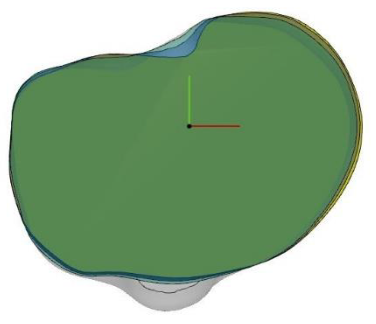
• Convergence Test: Results of the Convergence Test are exemplified for the Asian femur SSM. The effect of increasing the population size (to up to 112 patients) on the resulting average model is depicted Figure 3. Convergence is not achieved, as the mean RMS error does not reach zero before the populations begin to overlap (dotted line). However, with 80 patients (thus 24 overlapping scans), the error is less than 1.5 mm.

Figure 3. Mean RMS deviation between two Asian femur SSMs computed with different input data, for an increasing number of input patients (set size).

Figure 3. Mean RMS deviation between two Asian femur SSMs computed with different input data, for an increasing number of input patients (set size).

Leave-One-Out Analysis

Results of the leave-one-out study are exemplified for the Asian femur SSM. With 112 patients it was possible to predict patients with an RMS error below 1.5 mm using 15 modes of variation (Figure 4). Using all modes of variation, the model is able to predict patients with a mean accuracy of about 1 mm.

3.3. Use of the SSM

3.3.1. Definition of a Representative Database of 3D Bone Models

The AP/ML dimensions of the seven Caucasian bone models and the five Asian bone models lie in the middle of the cloud representing the AP/ML dimensions of the individual patients (Figure 5). The AP/ML dimensions of the seven Caucasian bone models ranged from (53.6/64.9 mm) for size 1 to (67.7/80.7 mm) for size 7. The AP/ML dimension of the five Asian bone models ranged from (53.0/62.4 mm) for size 1 to (60.5/72.4 mm) for size 5. The dimensions of the 10 additionally generated bones deviated from the target dimension on average (±1 standard deviation) by 0.2 ± 0.4 mm in AP and 0.5 ± 0.5 mm in ML. The maximum deviation was 0.9 mm in AP and 1.0 mm in ML. All 10 bones had a p-value of p < 10⁻²⁷.

3.3.2. Use of SSMs for Design Input

The tibia contours obtained by cutting the Caucasian tibia SSM orthogonally to the mechanical axis at 8, 10 and 12 mm are depicted in Figure 6.

The deepest points of the trochlea are depicted in Figure 7A. The resulting spline for one size is depicted in Figure 7B. Figure 7C shows the comparison of splines obtained with femurs of different sizes.

Splines of the center of the femoral canal in the frontal and sagittal planes were depicted for SSMs of different sizes (Figure 8) and are a useful input for defining the optimal curvature of long stems.

3.3.3. Use of SSMs for Design Validation

The shape of the patella resection and the position of the implant’s peak with respect to the native peak of the patella is shown on Figure 9. The peak is lateralized by 1.6 mm; the implant covers 75% of the resected surface.

The overhang and underhang of the Vega component are exemplified in Figure 10. This can well be analysed in 3D in all regions of the components.

4. Discussion

Statistical Shape Models are very interesting tools when analyzing the morphology in the population. They can be used for example to predict tibiofemoral kinematics [26], knee joint instability [27], or to quantify bony defects in hip revision surgery [28,29,30]. To our knowledge, there is no guideline on how to best use these models in the process of implant design. The aim of this study was to assess how to generate a valid SSM for implant design and to provide examples of how to use SSMs to evaluate the anatomic fit of TKA components. Those examples may contribute to the definition of guidelines on how to validate the anatomical fit of TKA components.

When generating a SSM for implant validation, it is crucial to analyze which input population should be used. For each application, a good compromise between homogeneity and size of the input population must be found. Gender and ethnicity have an important impact on the SSM and thus are distinguishable features in the populations. Therefore, it would be beneficial to examine the fit of the implant to SSMs built on different gender and ethnicities. In the present approach, it was decided to build two SSMs, one representing the Asian and the other the Caucasian population. The use of 120 Caucasian and 112 Asian anatomies, as well as the use of reference systems based on relevant anatomical landmarks, enabled robust SSMs. The fact that clinically relevant landmarks were used to define the reference systems greatly facilitated the use of the SSMs for design input and validation.

The crucial step to practically use the SSM for implant design was to generate a database of bone models out of the average SSMs. The seven Caucasian and five Asian bone models generated represented the average population well. Their AP/ML dimensions were located in the center of the cloud of points representing the AP/ML dimensions of the different patients. An additional 10 statistical models were computed to represent not only the average but also the patients with AP/ML dimensions at the borderline. Hence, a database of 22 bone models statistically well represented the Caucasian and Asian populations.

Various analyses can be performed on the database of bones to design and validate TKA implants. For design input, the outer shape of the proximal tibia is, for example, a key element to define the contour of the tibia plateau. Different studies compare the implant design with the anatomy of the population [16,17] by using a large number of CT scans of the input population. Algorithms are used to automatically place the components and evaluate their fit on all these anatomies. With the approach presented in the current study, the number of bone models included in the analysis could be drastically reduced by using bone models that statistically represent the population.

For the design of the anterior shield of the femoral component, the 3D geometry of the trochlea is an important input parameter which has been described in literature [31,32,33]. However, differences in the reference systems used make it difficult to compare these studies. Du [34] used 42 bone models to compare different trochlea designs. Our proposal to use a limited number of statistically relevant bone models is again a major advantage, as more anatomies are covered and less analyses are required. This also applies to the analysis of the overhang/underhang of the femoral component. Similarly, when looking at the patella, several studies have analyzed the morphology of the patella intraoperatively on several anatomies [10] or CT scans [35]. The bony coverage of various components could also be evaluated using a variety of patients’ anatomies [10,36]. The use of a limited database of statistically relevant bones allowed us to easily analyze the bony coverage and peak restoration of patella components on the input population.

One limitation of the models is that they represent the femur, patella, and tibia bones independently from each other. Knowing the relative position of the bones would be valuable information. An alternative would be to compute SSMs for the whole leg. That means building SSMs that comprise the tibia, the patella, and the femur. These SSMs can be valuable to analyze, for example, the relative size of the tibia and femur, or the relative alignment of the patella and the femur. However, the alignment of the bones is strongly influenced by the patient’s position during the CT scan. Since the patient is scanned lying on his back, this bone position does not necessarily match the knee in active conditions such as standing upright or being in flexion. For this reason, it would be interesting to work with 4D SSMs that include gait to capture the correct anatomical position and relative bone position during motion. This would also help us to link the models to the expected kinematics and allow to visualize and thereby better understand the kinematic of each patient’s joint. Another limitation is the lack of soft-tissue information, which limits the quality of the virtual implantation. Moreover, cartilage is not represented in the models if they are based on CT data. The SSMs presented in this paper were built on 112 and 120 CT datasets. This limits the power of the model to provide insight for specific parts of the population. For example, it is difficult to draw design conclusions for very small patients (such as, for example, the first percentile of the population). Additionally, since these tools are recent and rely on methods that most of the medical community are not familiar with, it can be very useful to complete this validation on individual anatomies.

5. Conclusions

The use of SSMs enables a detailed and very efficient evaluation of the anatomical fit of TKA designs. Few models suffice to represent the big variability in the population. Detailed 3D analysis can be performed. The key element is to build robust and valid models that can then be used to derive a database of bones. This set of bone models in various shapes and sizes statistically well represent the population. Different measurements can then easily be performed for design input or to check how well an implant fits these models, and hence the input population.

References

1. Bonnin, M.P.; Schmidt, A.; Basiglini, L.; Bossard, N.; Dantony, E. Mediolateral oversizing influences pain, function, and flexion after TKA. Knee Surg. Sports Traumatol. Arthrosc. 2013, 21, 2314–2324. [Google Scholar] [CrossRef] [PubMed] [Green Version]
2. Mahoney, O.M.; Kinsey, T. Overhang of the femoral component in total knee arthroplasty: Risk factors and clinical consequences. J. Bone Jt. Surg. 2010, 92, 1115–1121. [Google Scholar] [CrossRef]
3. Matz, J.; Lanting, B.A.; Howard, J.L. Understanding the patellofemoral joint in total knee arthroplasty. Can. J. Surg. 2019, 62, 57–65. [Google Scholar] [CrossRef] [Green Version]
4. Ng, J.W.G.; Bloch, B.V.; James, P.J. Sagittal radius of curvature, trochlea design and ultracongruent insert in total knee arthroplasty. EFORT Open Rev. 2019, 4, 519–524. [Google Scholar] [CrossRef]
5. Gu, S.; Kuriyama, S.; Nakamura, S.; Nishitani, K.; Ito, H.; Matsuda, S. Underhang of the tibial component increases tibial bone resorption after total knee arthroplasty. Knee Surg. Sports Traumatol. Arthrosc. 2019, 27, 1270–1279. [Google Scholar] [CrossRef]
6. Bonnin, M.; Saffarini, M.; Shepherd, D.; Bossard, N.; Dantony, E. Oversizing the tibial component in TKAs: Incidence, consequences and risk factors. Knee Surg. Sports Traumatol. Arthrosc. 2015, 24, 2532–2540. [Google Scholar] [CrossRef] [PubMed]
7. Chaichankul, C.; Tanavalee, A.; Itiravivong, P. Anthropometric measurements of knee joints in Thai population: Correlation to the sizing of current knee prostheses. Knee 2011, 18, 5–10. [Google Scholar] [CrossRef]
8. Cheng, F.B.; Ji, X.F.; Lai, Y.; Feng, J.C.; Zheng, W.X.; Sun, Y.F.; Fu, Y.W.; Li, Y.Q. Three dimensional morphometry of the knee to design the total knee arthroplasty for Chinese population. Knee 2009, 16, 341–347. [Google Scholar] [CrossRef] [PubMed]
9. Chung, B.J.; Kang, J.Y.; Kang, Y.G.; Kim, S.J.; Kim, T.K. Clinical Implications of Femoral Anthropometrical Features for Total Knee Arthroplasty in Koreans. J. Arthroplast. 2015, 30, 1220–1227. [Google Scholar] [CrossRef]
10. Yang, C.C.; Dennis, D.A.; Davenport, P.G.; Kim, R.H.; Miner, T.M.; Johnson, D.R.; Laz, P.J. Patellar component design influences size selection and coverage. Knee 2017, 24, 460–467. [Google Scholar] [CrossRef] [Green Version]
11. Morris, W.Z.; Gebhart, J.J.; Goldberg, V.M.; Wera, G.D. Implant Size Availability Affects Reproduction of Distal Femoral Anatomy. J. Knee Surg. 2016, 29, 409–413. [Google Scholar] [CrossRef]
12. Dai, Y. (Ed.) Distal Femoral Morphology and Its Correlation with Two Contemporary TKA Designs. In Proceedings of the ORS 2017 Annual Meeting, San Diego, CA, USA, 19–22 March 2017. [Google Scholar]
13. Ha, C.W.; Na, S.E. The correctness of fit of current total knee prostheses compared with intra-operative anthropometric measurements in Korean knees. J. Bone Jt. Surg. Br. Vol. 2012, 94, 638–641. [Google Scholar] [CrossRef] [PubMed]
14. Hitt, K.; Shurman, J.R.; Greene, K.; McCarthy, J.; Moskal, J.; Hoeman, T.; Mont, M.A. Anthropometric measurements of the human knee: Correlation to the sizing of current knee arthroplasty systems. J. Bone Jt. Surg. Am. Vol. 2003, 85 (Suppl. S4), 115–122. [Google Scholar] [CrossRef] [Green Version]
15. Lonner, J.H.; Jasko, J.G.; Thomas, B.S. Anthropomorphic differences between the distal femora of men and women. Clin. Orthop. Relat. Res. 2008, 466, 2724–2729. [Google Scholar] [CrossRef] [PubMed] [Green Version]
16. Clary, C.; Aram, L.; Deffenbaugh, D.; Heldreth, M. Tibial base design and patient morphology affecting tibial coverage and rotational alignment after total knee arthroplasty. Knee Surg. Sports Traumatol. Arthrosc. 2014, 22, 3012–3018. [Google Scholar] [CrossRef] [PubMed] [Green Version]
17. Dai, Y.; Bischoff, J.E. Comprehensive assessment of tibial plateau morphology in total knee arthroplasty: Influence of shape and size on anthropometric variability. J. Orthop. Res. 2013, 31, 1643–1652. [Google Scholar] [CrossRef]
18. Cootes, T.; Taylor, C.J. Statistical Models of Appearance for Computer Vision; University of Manchester: Manchester, UK, 2004. [Google Scholar]
19. Kellgren, J.H.; Lawrence, J.S. Radiological assessment of osteo-arthrosis. Ann. Rheum. Dis. 1957, 16, 494–502. [Google Scholar] [CrossRef] [PubMed] [Green Version]
20. Akagi, M.; Oh, M.; Nonaka, T.; Tsujimoto, H.; Asano, T.; Hamanishi, C. An Anteroposterior Axis of the Tibia for Total Knee Arthroplasty. Clin. Orthop. Relat. Res. 2004, 420, 213–219. [Google Scholar] [CrossRef]
21. Franceschini, V.; Nodzo, S.R.; Della Gonzalez Valle, A. Femoral Component Rotation in Total Knee Arthroplasty: A Comparison between Transepicondylar Axis and Posterior Condylar Line Referencing. J. Arthroplast. 2016, 31, 2917–2921. [Google Scholar] [CrossRef] [PubMed]
22. Kobayashi, H.; Akamatsu, Y.; Kumagai, K.; Kusayama, Y.; Ishigatsubo, R.; Muramatsu, S.; Saito, T. The surgical epicondylar axis is a consistent reference of the distal femur in the coronal and axial planes. Knee Surg. Sports Traumatol. Arthrosc. 2014, 22, 2947–2953. [Google Scholar] [CrossRef]
23. Victor, J.; van Doninck, D.; Labey, L.; van Glabbeek, F.; Parizel, P.; Bellemans, J. A common reference frame for describing rotation of the distal femur: A ct-based kinematic study using cadavers. J. Bone Jt. Surg. Br. 2009, 91, 683–690. [Google Scholar] [CrossRef] [Green Version]
24. Dupraz, I.; Jacobs, M.; Deckx, J.; Firmbach, F.-P.; Utz, M. Mise en Place d’un Référentiel Anatomique sur un Modèle Statistique de la Rotule; Livre des résumés des communications de la SOFCOT: Paris, France, 2019. [Google Scholar]
25. Dai, Y.; Scuderi, G.R.; Penninger, C.; Bischoff, J.E.; Rosenberg, A. Increased shape and size offerings of femoral components improve fit during total knee arthroplasty. Knee Surg. Sports Traumatol. Arthrosc. 2014, 22, 2931–2940. [Google Scholar] [CrossRef] [Green Version]
26. van Dijck, C.; Wirix-Speetjens, R.; Jonkers, I.; Vander Sloten, J. Statistical shape model-based prediction of tibiofemoral cartilage. Comput. Methods Biomech. Biomed. Eng. 2018, 21, 568–578. [Google Scholar] [CrossRef]
27. Cerveri, P.; Belfatto, A.; Manzotti, A. Predicting Knee Joint Instability Using a Tibio-Femoral Statistical Shape Model. Front. Bioeng. Biotechnol. 2020, 8, 253. [Google Scholar] [CrossRef] [PubMed]
28. Vanden Berghe, P.; Demol, J.; Gelaude, F.; Vander Sloten, J. Virtual anatomical reconstruction of large acetabular bone defects using a statistical shape model. Comput. Methods Biomech. Biomed. Eng. 2017, 20, 577–586. [Google Scholar] [CrossRef]
29. Schierjott, R.A.; Hettich, G.; Graichen, H.; Jansson, V.; Rudert, M.; Traina, F.; Weber, P.; Grupp, T.M. Quantitative assessment of acetabular bone defects: A study of 50 computed tomography data sets. PLoS ONE 2019, 14, e0222511. [Google Scholar] [CrossRef] [Green Version]
30. Hettich, G.; Schierjott, R.A.; Ramm, H.; Graichen, H.; Jansson, V.; Rudert, M.; Traina, F.; Grupp, T.M. Method for quantitative assessment of acetabular bone defects. J. Orthop. Res. 2019, 37, 181–189. [Google Scholar] [CrossRef] [PubMed]
31. Nascimento, S.R.R.; Pereira, L.A.; Oliveira, M.J.; Wafae, G.C.; Ruiz, C.R.; Wafea, N. Morphometric analysis of the angle of the femoral trochlea. J. Morphol. Sci. 2011, 28, 250–254. [Google Scholar]
32. Iranpour, F.; Merican, A.M.; Dandachli, W.; Amis, A.A.; Cobb, J.P. The geometry of the trochlear groove. Clin. Orthop. Relat. Res. 2010, 468, 782–788. [Google Scholar] [CrossRef] [PubMed] [Green Version]
33. Monk, A.P.; Choji, K.; O’Connor, J.J.; Goodfellow, J.W.; Murray, D.W. The shape of the distal femur: A geometrical study using MRI. Bone Jt. J. 2014, 96, 1623–1630. [Google Scholar] [CrossRef] [PubMed]
34. Du, Z.; Chen, S.; Yan, M.; Yue, B.; Wang, Y. Differences between native and prosthetic knees in terms of cross-sectional morphology of the femoral trochlea: A study based on three-dimensional models and virtual total knee arthroplasty. BMC Musculoskelet. Disord. 2017, 18, 166. [Google Scholar] [CrossRef] [PubMed]
35. Huang, A.-B.; Luo, X.; Song, C.-H.; Zhang, J.-Y.; Yang, Y.-Q.; Yu, J.-K. Comprehensive assessment of patellar morphology using computed tomography-based three-dimensional computer models. Knee 2015, 22, 475–480. [Google Scholar] [CrossRef] [PubMed]
36. Ali, A.; Long, J.; Wright, A.; Clary, C.W. The Shape of the Resected Patella and Design Factors Affecting Patella Coverage and Restoration of Patella Anatomy. In Proceedings of the ORS 2014 Annual Meeting, New Orleans, LA, USA, 28–29 April 2014. [Google Scholar]
Figure 1. Generated Caucasian and Asian bone models.
Applsci 12 01020 g001
Figure 2. Comparison between average SSMs of the healthy and arthritic bones (femur/tibia/patella). Positive values mean the average arthritic model is larger than the average healthy model.
Applsci 12 01020 g002aApplsci 12 01020 g002b
Figure 4. Average RMS deviation between the 112 Asian Femur SSMs computed by leaving each patient out once, with an increasing number of modes. The error bars indicate the standard deviations.
Applsci 12 01020 g004
Figure 5. AP/ML dimensions on the Caucasian and Asian population, the SSM and the 10 additionally generated statistical models.
Applsci 12 01020 g005
Figure 6. Contour of the tibia plateau cut at 8 (dark green), 10 (blue) and 12 mm (light green).
Applsci 12 01020 g006
Figure 7. (A) Trochlea extracted on a Statistical Shape Model; (B) spline of the Trochlea projected on the sagittal plane; (C) comparison of trochlea splines for 3 SSM sizes.
Applsci 12 01020 g007
Figure 8. (A) Spline of the femoral canal; (B) splines of different sized SSMs (sagittal view); (C) splines of different sized SSMs (frontal view).
Applsci 12 01020 g008
Figure 9. Statistical Shape Model of Patella resected at 6 mm and implanted with a universal patella (Aesculap, Tuttlingen, Germany). The implant peak (red) is 1.6 mm lateralized with respect to the native patella peak (blue).
Applsci 12 01020 g009
Figure 10. (A): Underhang of the femoral component in the frontal view. The underhang is most important on the lateral side of the anterior shield. (B): Underhang of the femoral component in the axial view. The underhang is most important on the medial side of the distal cut.
Applsci 12 01020 g010
Publisher’s Note: MDPI stays neutral with regard to jurisdictional claims in published maps and institutional affiliations.