Abstract
Geophysical techniques are widely applied in the archaeological field to highlight variations of the physical behaviour of the subsoil due to the presence of ancient and buried remains., Considerable efforts are required to understand the complexity of the relationship between archaeological features and their geophysical response where saturated conditions occur. In the case of lacustrine and wetland scenarios, geophysical contrasts or electromagnetic signal attenuation effects drastically reduce the capabilities of the geophysical methodologies for the detection of structures in such conditions. To identify the capability of the electrical and electromagnetic methods in different water-saturated scenarios, an experimental activity was performed at the Hydrogeosite CNR laboratory. The test allowed us to analyze the limits and potentialities of an innovative approach based on the combined use of the ground-penetrating radar and 2D and 3D electrical resistivity tomographies. Results showed the effectiveness of the ground-penetrating radar for detecting archaeological remains also in quasi-saturated and underwater scenarios despite the em signal attenuation phenomena; whilst the results obtained involving the resistivity tomographies offered a new perspective for the archaeological purposes due to the use of the loop–loop shaped array. Moreover, the radar signal attenuation, resolution and depth of investigation do not allow to fully characterize the archaeological site as in the case of the scenarios with a limited geophysical contrast (i.e., water-saturated and arid scenarios). The experimental tests show that these limits can be only partially mitigated through the integration of the geophysical methodologies and further efforts are necessary for improving the results obtainable with an integrated use of the adopted geophysical methodologies.
1. Introduction
Among various active geophysical techniques, electric and electromagnetic (em) methods are strongly effective for the detection of archaeological features located in the subsoil at different depths and scenarios [1,2,3,4,5,6,7]. Localization of anthropic structures placed in the soil is possible due to the contrast of the em physical properties between the materials constituting the buried objects and the subsoil where they are “preserved”. The presence of the “geophysical contrast” between the analyzed structures and background soil represents the necessary conditions for successful research in the archaeogeophysical field. However, the presence of subsoil with a high-water content (close to the saturation) could be a limit for the research due to em signal attenuation problems and “homogenization effect” of the subsoil physical behaviour. From one side, the attenuation phenomena related to a high water and clay content of the soil play a crucial role for the em methodologies and strongly influence the depth of investigation, resolution, and velocity of propagation [8]. From the other side, a homogenous electrical behaviour of the subsoil due to high water content, also in presence of archaeological features, could be a hard problem for the resistivity techniques. Moreover, despite limitations caused by the presence of water, em and electrical geophysical prospecting are often the only way that can support archaeologists to identify interesting areas to excavate. Additionally, archaeogeophysical investigations in underwater conditions today represent one of the most interesting challenges for the geophysical applications [9]. In this fascinating field, the geophysical methods have been fast developing in the last two decades and, regarding the sub-water archaeological surveys, the use of acoustic (sound or sonar) systems in well-established [10]. These include echo-sounders, multi-beam swath systems, side-scan sonars, sub-bottom profilers, and bottom classification systems. Nevertheless, notwithstanding the great depth of investigation, these methods are characterized by a low resolution; therefore, in scenarios with fresh water, great attention is addressed to the investigations of underwater structures with high resolution techniques, among which stands out the ground penetrating radar (GPR) [11,12,13], joint to other methodologies such as direct current (DC) electrical resistivity method.
The use of GPR in water covered areas is still a challenge because it suffers a series of problems linked to the em signal attenuation in the presence of water. However, it has been successfully used to detect geological structures and archaeological features beneath see, rivers, ponds, and swamps bottom [14,15,16,17,18]. In general, the surveys were carried out using small boats and antennas with frequencies between 100 and 400 MHz.
On the contrary, electrical resistivity methods are more commonly used in water covered areas (stream, river, wetland, lake, and sea), for evaluating subsurface conditions for hydrogeological and environmental purposes [19,20]. Rarer are applications in the maritime archaeological field [21,22]. In general, surveys in water-covered areas include conventional surveys using a multi-electrode resistivity system where part of the survey line crosses a river or a lake, and surveys conducted entirely within a water-covered environment. In applications in seas and rivers, this method has been performed both with fixed electrodes placed on the water surface or on the seabed and riverbed [23,24,25,26,27,28,29] or by dragging the electric cable on the water surface with the aid of ships or boats [30,31]. In the first case, usually, the cable is weighted in order to allow direct contact with the marine sediments. The use of floating cables allows to cover a wider area; however, measurement errors may be higher due to the stacking suppression, off-line array movement induced by boat navigation, wind, or wave action, electrode cavitation at high boat speeds, and vegetation entrainment on electrodes. Usually, streamer electrodes can be made of steel or graphite; however, the latter are more fragile but more resistant to saltwater corrosion [24]. Less common are electrical resistivity measurements in water-covered areas such as wetlands, ponds, and lakes [31,32,33,34].
One strategy to improve the resolution of electrical resistivity tomograms in water covered areas is to incorporate constraints on the water-column resistivity and thickness. In particular, the electrical resistivity of the water, in the margins of eligible error, can be considered constant [35].
In this framework, the main goal of our research consists of the preliminary analysis of the contribution of the two different geophysical methods, direct current (DC) and GPR offer for archaeogeophysical purposes, unsaturated and underwater scenarios (i.e., lacustrine, wetlands, underwater landslide, and fast natural erosion coast).
For these aims, an archaeological site was reconstructed at the Hydrogeosite laboratory [36] with buried full-scale archaeological remains and different water content conditions were reproduced. The archaeological test site was characterized by remains simulating structures of the Lucanian and Roman times (walls, tombs, roads, etc.) covered by sediments [37,38,39,40]. The approach adopted is based on the cooperative use of GPR and electrical resistivity tomography (ERT), adopting 2D and 3D data acquisition strategies. The paper defines different GPR and DC conventional and non-conventional acquisition procedures, in order to highlight the best setting in water saturated/quasi-saturated subsoil and flooded conditions, and a first level of integration is shown. In particular, we applied GPR on a boat and ERT on the water to demonstrate the potentiality of the methods applied in tandem for shallow underwater research. Further, the effectiveness of the non-conventional loop–loop array for ERT analyses was analyzed and compared with classical setting. With the loop-shaped acquisition scheme, we have tried to overcome the limitations analysing the effective capacity of the DC method. The qualitative integration of the GPR and ERT data has been tried in order to reduce the uncertainties for the archaeological features detection and preliminary quantitative analyses of the geophysical data regarding the real sizes and positions of the buried objects, which are discussed in this paper.
The outline of this paper is as follows. After a brief overview of GPR and ERT is applied to the archaeological field, a description of the archaeological test site is shown. Then, the results obtained in two main phases of the experiments are presented and discussed. Finally, conclusions and future perspectives are debated in the last paragraph.
2. Theoretical Notes
Geophysical techniques have become of crucial importance in the preliminary phase of archaeological site detection and mapping; indeed, they are able to provide quick and inexpensive high-quality information on the presence and distribution of remains in many different archaeological scenarios. The probability of a successful application rapidly increases if multi-methodological approaches are adopted, according to a logic of objective complementarity of information and global convergence toward a high quality multi-parametric imaging of the buried structures [41].
In detail, GPR represents an excellent tool to support the archaeologists to identify and reconstruct the real geometry of the objects located in the soil. The GPR lies in electromagnetic (em) theory where the full electromagnetic field is mathematically described by Maxwell’s equations. GPR allows for the study of the scattering phenomena of em waves caused by variations of some physical properties of the investigated medium as dielectric permittivity (ε, F/m), electrical conductivity (σ, S/m), and magnetic permeability (μ, H/m). These physical variations generate reflections related to contrasts in the em impedance; further, the em properties of the soil barely influence the velocity of propagation of em waves and the attenuation of the energy introduced in the subsoil. In low-loss conditions, velocity and the attenuation of em waves can be approximated as follows [42]:
where is the velocity of light in a vacuum (m/s), and are the magnetic permeability (4π × 10−7 H/m) and dielectric permittivity (8.854 × 10⁻¹² F/m) in the free space and the dielectric constant (dimensionless) with magnetic permeability considered negligible and ε the dielectric permittivity of the medium (F/m).
The above two expressions show that the dielectric permittivity (ε) controls em wave velocity, while the electrical conductivity () has a large effect on attenuation. For this reason, GPR works well where the soil conductive is low [42,43,44,45].
Nowadays, GPR is probably one of the most used non-invasive geophysical techniques in the archaeological field witnessed by an increasing amount of scientific research published in the last four decades [7,45,46,47,48,49,50,51,52,53,54,55,56,57,58,59,60,61,62,63].
Direct current (DC) electrical methods are among the oldest and most popular techniques for the non-invasive geophysical investigations. Among them, ERT allows to investigate the horizontal and vertical electrical resistivity variations of the subsurface materials potentially induced by the presence of anomalous bodies.
DC method is based on the measurement of an electric field artificially created in the ground with suitable electronic devices; it normally consists of two pairs of electrodes fixed in the ground, of which: a pair constitutes the current injection circuit, the other the measuring circuit of the potential difference (dV) generated in the ground by the passage of the current itself. The fundament of this technique is Ohm’s Law, which indicates that the potential difference dV (V) at the ends of a conductor, at a given temperature T, is proportional to the electric current I (A) passing through it by means of a quantity constant and typical of the conductor, said resistance R (Ω):
where ρ (Ωm) is the electrical resistivity, L (m) is the conductor length, and A (m2) is the conductor area. Generally, a switched square wave is the current waveform used [64]. The data acquired are expressed in form of apparent resistivity (ρa)
where ΔV (V) is the measured potential, I (A) the transmitted current, and K (m) the geometric factor, which depend on the position of electrodes. It is possible to define different configuration: Wenner, Shlumberger, dipole–dipole, gradient arrays, pole–pole, pole–dipole. Moreover, due to new acquisition instruments with a high number of channels, it is possible to make a personal disposal of the electrodes with different regular or irregular geometry [65]. The apparent resistivity is then interpreted in terms of real resistivity and depth by means of inversion software. The aim of the inversion procedure is to compute the ‘best’ set of resistivity values, which satisfies both the measured dataset and some a priori constraints, in order to stabilize the inversion and constrain the final image [66,67]. However, the method is affected by limitations mainly due to the resolution and time to perform the investigations. In the past, 2D ERTs were successfully used for archaeological prospecting [68,69,70,71,72,73,74,75,76,77,78]. Furthermore, several authors have effectively performed 3D ERT applied in the archaeological field to detect the excavation of buried structures [1,78,79,80,81,82,83]. Resistivity methods, including ERT, are less used then GPR in archaeological surveys for the limited resolution, but in the presence of conductive context as in the case of soils with high content of water, salt water or clay), they could be a good alternative to the GPR that suffers attenuation problems. Furthermore, an integration and a comparison of the results obtained via the two techniques is a preferable approach to support archaeologists and enhance the quality of the interpretation of the geophysical data as showed by the existing literature [1,84,85,86,87,88].
ρa = ΔV/IK
3. Materials and Methods
3.1. The Full-Scale Archaeologeophysical Test
The experiment was realized at the Hydrogeosite laboratory (CNR-IMAA Marsico Nuovo -PZ), where a concrete pool of 250 m3 (12 × 7 × 3 m) is located (Figure 1). The pool is filled with silica sand (95% SiO2) characterized by an average diameter equal to 0.09 mm (very fine sand), a porosity of about 45–50%, and a hydraulic conductivity of about 10−5 m/s (see Table 1).
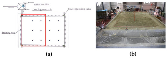
Figure 1.
The operating system of the concrete pool used for hydrogeophysical experiments at the Hydrogeosite laboratory (a) and an aerial photo of the investigated site (b).

Table 1.
Particle size analysis and chemical and hydraulic parameters of the homogeneous sand used at the Hydrogeosite laboratory.
The pool is equipped with 17 wells and a hydraulic system (draining ring system) for the reproduction of a phreatic aquifer that allows the variation of groundwater level (Figure 1a).
In this context, an archaeological site was reconstructed and buried by sand and different water content conditions were reproduced in order to simulate wet and lacustrine conditions typical of wetlands even assuming extreme events (for example, submarine landslide or fast coast natural erosion). For this experiment, a limited area of 6 m × 4 m (Figure 1b) inside the large pool was selected, and the archaeological features were buried until a depth of about 1.50 m from the original ground surface.
After the excavation activities, the area was filled with moist sand to obtain a quite homogeneous filling. We have proceeded layer by layer regularly compacting the sand by several cycles of tap water charge and discharge, from the bottom to the surface. In order to make the reconstruction as faithful as possible to real case, a study on the historical and archaeological area was carried out, taking in account the material used, the construction types, and techniques and methods of materials. The archaeological context was obtained following the dictates reported by ancient sources as those set forth by Vitruvio (De Architectura) and several studies published over time [89,90,91,92,93,94,95,96,97]. We adopted stylistic and structural elements belonging to different historical periods, places, and ethnos that find their coexistence in the middle Republican age and in the late-Imperial phase but even employed in more recent times, such as the capuchin tombs and ‘box-grave’ composed of large clay tegulae (tiles) used in the IV-III B. C. century but also in the Imperial period, or the opus coementicium (i.e., a hydraulic mortar laid in alternate courses with aggregate) continuously employed from its invention to the present time. In detail, it was involved in the construction of two different areas for the living context and funerary world, as shown in Figure 2b. A marble column, a capuchin burial, and a tiles burial were placed, as shown in Figure 2c along the S1 section (from left to right). Instead, along the S2 section as shown in Figure 2d (from left to right), part of a building and a paved road fragment were constructed. The building, defined by two dividing walls converging to form a corner, had incorporated a floor covered with mosaic; in this case, a small collapse near the structure was simulated. In Table 2, the electrical and em properties of the archaeological elements and background soil are presented.
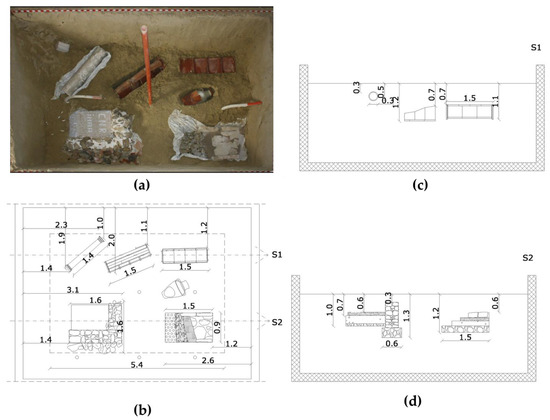
Figure 2.
The archaeological framework reconstructed in the laboratory: (a) plan of remains (b) and transversal sections S1 (c) and S2 (d). The circles shown in the maps represent the positions of the piezometers and the numbers indicate the distance in meters. The pool is 12 m × 7 m × 3 m.
Table 2.
Electrical and em properties of the archaeological elements and background soil.
The experiment consisted of two main working phases (WP):
- WP1: top of the shallower structures placed at 0.30 m from the original surface (Figure 3a);
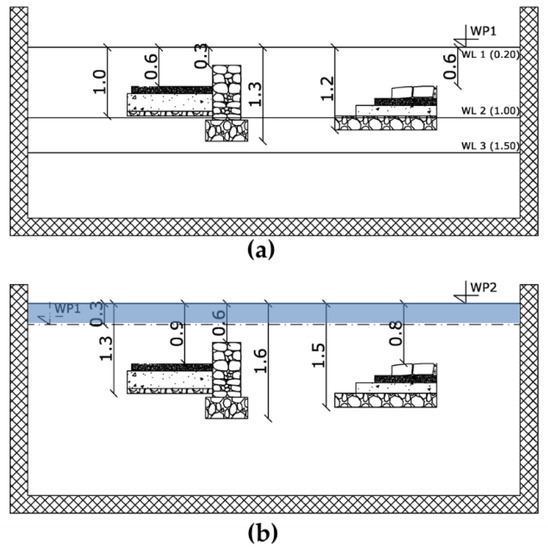 Figure 3. Two WPs were investigated: (a) WP1 with the water table placed at three different depths (respectively fixed to 0.20 m (WL1), 1.00 m (WL2) and 1.50 m (WL3); and (b) WP2, with the archaeological site covered by a water column of 0.3 m. The numbers indicate the distances in meters.
 - WP2: all the site was covered by water to reproduce an underwater archaeological site (Figure 3b).
In WP1, the water level (WL) was placed at three different heights equal to 0.20 m (WL1), 1.00 m (WL2), and 1.50 m (WL3) from the surface of investigation (Figure 3a), while in WP2 the surveys were performed in the presence of a water column of 0.3 m above the sand surface (Figure 3b). The entire experiment was realized with the use of tap water characterized by the electrical resistivity value of about 30 Ωm.
3.2. Geophysical Surveys
Geophysical surveys were performed with the use of the SIR-3000 TerraSurveyor (GSSI System) ground penetrating radar (Figure 4a) and Syscal Pro Switch 96 (Iris Instruments) georesistivimeter (Figure 4b). Data acquisition and processing were set considering the two different scenarios related to WP1 (Figure 4a,b) and WP2 (Figure 4c,d).
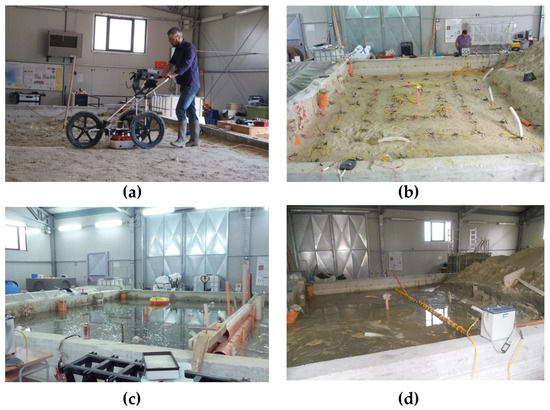
Figure 4.
GPR Sir 3000 and 400 Mhz antenna with survey wheel: (a) loop–loop ERT acquisition system (b) performed in WP1 (unsaturated scenarios), 400 Mhz GPR antenna on a small boat, and (c) a 2D ERT profile with floating electrode (d) in WP2 (underwater scenario).
In detail, GPR surveys were carried out in WP1 using a reference grid where the distance from each line was equal to 0.20 m and the investigations were made in both the main directions (red arrows in Figure 5a). In WP2, the presence of the water did not allow the 3D acquisition and only the two sections S1 and S2 were investigated (Figure 5c). In this case, the antenna was placed on a small boat dragged with pulleys fixed at the concrete wall of the pool to allow for the collection of the data without the use of an odometer. A marker every 0.075 m was imposed for assigning the real position to the acquired traces. All the data were acquired in continuous and reflection mode with the two-time window of 70 ns at the frequency of 400 MHz. The scan samples were set at 512 with a resolution of 16 bits and a transmission rate of 100 KHz.
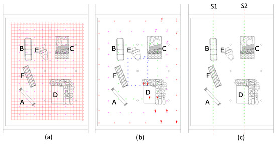
Figure 5.
Acquisition grid used to collect GPR data and the location of the electrodes for dipole–dipole acquisition in WP1: (a) the red arrows indicate the GPR acquisition direction, while the coloured circles individuate the position of the electrodes; (b) the loop–loop 3D ERT was defined with the electrodes located along four loops with different electrode distances; (c) the lines investigated with the GPR and ERT in WP2, the green circles indicate the position of the electrodes.
GPR data processing consisted of the use of some basic operations, including band-pass filters, gain function removal, amplitude compensation, background removal filter, and Kirchhoff migration. To migrate the data, the em velocity evaluation was performed, studying the diffraction hyperbolas generated by the archaeological features that was constantly varied due to the raising of the water table. In order to detect and reconstruct the archaeological remains, after the examination of the individual radargrams, 3D data volumes were created and some significative time slices, converted in depth slices, were extracted to identify the buried structures. In WP2, it has been necessary to add a further step for the data editing, including the association of the real position to the traces acquired without the use of the odometer.
Regarding the ERT acquisitions in WP1, 3D ERTs were performed with the use of two different types of 3D arrays. In detail, a 3D acquisition based on a grid of 96 steel electrodes (pink circles in Figure 5a) distributed on an area of 7 × 4 m was adopted. First, 3D pseudo resistivity data were collected using dipole–dipole array with in-line, parallel-line and diagonal-line dipoles; the electrode spacing was 0.60 m in both the directions. Further, a 3D non-conventional array with a loop shaped (loop–loop array) was used: both current (C+ and C−) and potential (V+ and V−) electrodes were distributed along the entire site surface according to four concentric rings (Figure 5b). In the outer ring (red circles), the electrodes were placed at a reciprocal distance of 1.00 m; in the second ring (magenta circles), the mutual distance was 0.75 m; for the last two inner rings, the distances were 0.50 (green circles) and 0.25 m (blue circles), respectively.
In WP2, where underwater scenarios have been simulated, 2D ERTs were carried out with electrodes placed both on the underwater floor and on the water surface by a floating system, which was realized ad hoc. In addition, only the S1 and S2 sections were investigated (Figure 5c).
ERT data were processed by means of an inverse modelling software according to an iterative process, which aims at minimizing the difference between the measured pseudo-section and the calculated pseudo-section based on a starting model. In detail, apparent resistivity data inversion of 3D ERT was performed using ERTLab software using a quadrilateral mesh. The inversion procedure is based on a smoothness constrained least-squared algorithm with Tikhonov model regularization, where the condition of the minimum roughness of the model is used as a stabilizing function. [98]. The 2D inversion was carried out with the ResIPy open-source software [99]. In this case, a confined rectangular mesh was used for considering the presence of the concrete walls of the pool. Moreover, in WP2, the presence of the water column has necessarily required the optimization of the starting forward model by considering, above the sand body, the presence of a 30 cm thick layer with constant electrical resistivity value equal to 30 Ωm.
4. Results
4.1. WP1—Unsaturated Scenarios
4.1.1. GPR Results in WP1
In WP1, the depth of the shallower archaeological structures was about 0.20 m, corresponding to the top of the column and stone wall. The drier scenario (WL3), with the water table deep 1.50 m, is characterized by the em velocity of 0.17 mns−1 equivalent to a εr of 2.8. The reflections imputable to the column (A), stone wall (D), rectangular tomb (B), and paved road (C) are clearly detectable (Figure 6). Regarding the size of the highly reflective bodies, there is a good agreement between the reflective areas and the presence of the structures, especially for the column and the wall. Some difficulties are related to the localization of the capuchin tomb (F) and enchytrismos (E) that are not clearly detectable for to their geometrical sizes and orientation. Further some reflections not associable to the structures, due to a low soil compaction, have caused a blurry image of the buried objects.
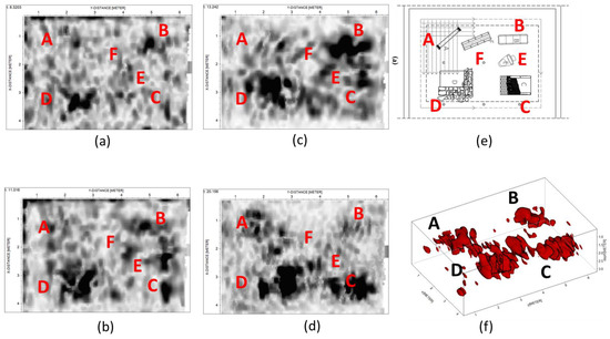
Figure 6.
Time-slices at the depths of 0.25 m (a), 0.45 m (b), 0.70 m, and (c) 1.00 m (d) with a water table at a depth of 1.50 m (WL3). In (f) the 3D iso-amplitude volumes obtained selecting only the highest reflections; (e) the plane of the test site.
The intermediate scenario (WL2) with the water table at a depth of 1.00 m (structures partially underwater) is characterized by the em velocity of 0.15 mns−1 equivalent to a εr of 4.0. The results obtained with WL2 are shown in Figure 7. It is interesting to note how the reflections related to the objects are weakened at the depth of one meter for the attenuation of the signal. The capuchin tomb (F) is not easily recognizable, while the enchytrismos (E) is not identifiable. The rectangular tomb (B), the paved road (C), and the wall corner (D) are detectable; moreover, the last structure is well-defined and focused, because the increase of the water content degree has induced a better compaction of the ground and some reflections caused by the excavation activities, visible in the previous case, disappear.
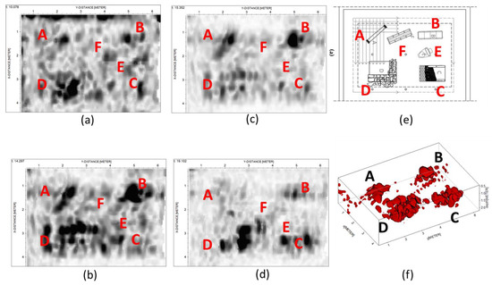
Figure 7.
Time-slices at the depths of 0.25 m (a), 0.45 m (b), 0.70 m (c), and 1.00 m (d) with a water table at a depth of 1.00 m (WL2); (f) the 3D iso-amplitude volumes obtained selecting only the highest reflections; (e) the plane of the test site.
The third step was obtained with the water table level fixed at 0.20 m (WL1). This is the wetter scenario characterized by a em velocity of 0.07 mns−1 equivalent to a εr of 18.5. The results shown in Figure 8 highlight unequivocally the attenuation imputable to the fact that the objects are all underwater. Indeed, only the column (A), the top of the wall (D), the rectangular tomb (B), and the enchytrismos (E) are clearly detectable, whilst the capuchin tomb (F) and the paved road (C) are not easily detectable.
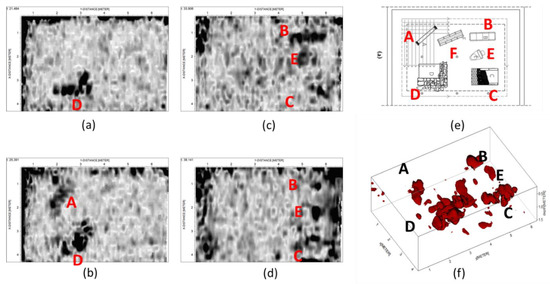
Figure 8.
Time-slices at a depth of 0.25 m (a), 0.45 m (b), 0.70 m, (c) and 1.00 m (d) with a water table 0.20 m (WL1); (f) the 3D iso-amplitude volumes obtained selecting only the highest reflecions and in (e) the plane of the test site.
4.1.2. ERT Results in WP1
As shown in Figure 9, the resistivity values obtained with the use of the 3D-ERTs range between 2 and 200 Ωm. The low values of resistivity are due to the presence of a high-water content in the sand while the greater values are induced by the presence of the archaeological remains. The resistivity distribution acquired with the classical 3D ERT configuration is not associated well to the buried archaeological structures, both in the drier scenario (Figure 9a) and the wetter scenario (Figure 9b). On the contrary, the loop–loop array provided an enhanced information regarding their distribution and shape (Figure 9c,d). In fact, several resistivity anomalies are well detected in the loop–loop 3D ERT image and they clearly highlight the presence of the corner wall (D), the capuchin tomb (F), and enchytrismos (E), as shown in the wetter scenario WL2 (Figure 9d). Less evident is the presence of the other structures that are located at the edges of the investigated area (column A and rectangular tomb B) or at a greater depth, as in the case of the paved road (C).
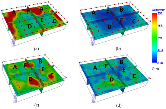
Figure 9.
3D ERTs acquired with the classical dipolar approach (upper figure) and loop–loop array (lower figure) in WL3 (a,c) and WL2 (b,d), respectvely. The cross section between the horizontal slices and the vertical ones is 0.5 cm.
The comparison of the results obtained with the two approaches shows the importance of the results obtained with the less conventional loop–loop shaped array, also highlighted by the depth slices extracted in the three different scenarios (Figure 10, Figure 11 and Figure 12). In detail, the slices extracted at increasing depths from the resistivity model in WL3 (drier scenario) allow to detect at least five of the six structures buried in the subsoil (Figure 10) despite the apparent noise in the shallower layer of the subsoil, induced by the excavation activities and bad compaction of the soil (Figure 10a). Increasing the depth, the presence of the structures is more easily detectable, as in the case of the corner wall (D) and the paved road (C) (Figure 10b,c). At the depth of 1.00 m, no structures are detectable for the scarce resolution of the method imputable to the few measurement points available.
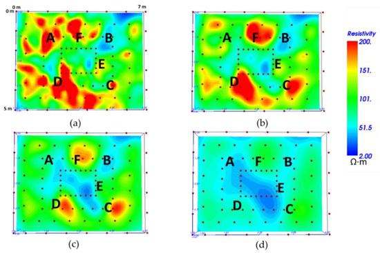
Figure 10.
3D loop–loop ERT depth-slices at 0.25 m (a), 0.45 m (b), 0.70 m (c), and 1.00 m (d) at WL3.
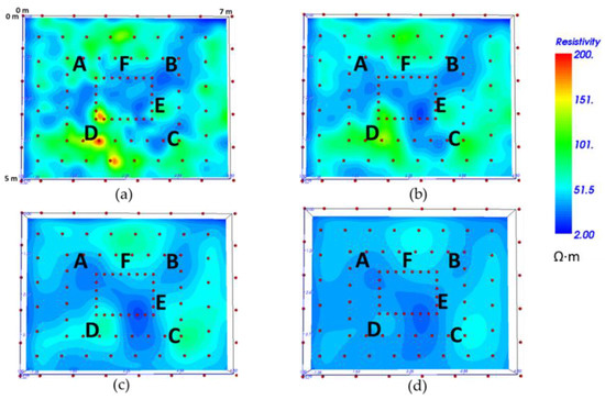
Figure 11.
3D loop–loop ERT depth-slices at 0.25 m (a), 0.45 m (b), 0.70 m (c), and 1.00 m (d) in WL2.
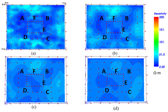
Figure 12.
3D loop–loop ERT depth-slices at 0.25 m (a), 0.45 m (b), 0.70 m (c), and 1.00 m (d) in WL1.
The results obtained with the water table at the depth of 1.00 m (in WL2) allow to detect a lower noise in the shallowed layers due to the higher water content in the subsoil (Figure 11), resulting in an improved geophysical contrast between the archaeological structures (more resistive) and background soil (more conductive). As in the previous case, apart from the rectangular tomb (B), the electrical anomalies can be associated for position and shape to the buried structures at the depths of 0.25 m (Figure 11a), 0.45 m (Figure 11b), and 0.70 m (Figure 11c).
In WL1 (Figure 12), the high water content does not permit the identification of electrical anomalies associated to the buried structures in any slices.
4.2. WP2—Underwater Scenario
In this phase, the underwater archaeological scenario has been analyzed. The experiment was setup by simulating a water column of 30 cm above the sand surface. In correspondence of the S1 and S2 transects, 2D GPR was performed above the water surface while ERTs were carried out above and below the water column.
GPR results are shown in Figure 13. In this case, the signal attenuation is greater than the previous conditions (WP1). However, it is possible to easily detect the location and the shape of the buried archaeological structures. The em velocity was equal to 0.035 mns−1 for the water layer (εr-w ≈ 81) and 0.065 mns−1 for the water saturated sand (εr ≈ 25).
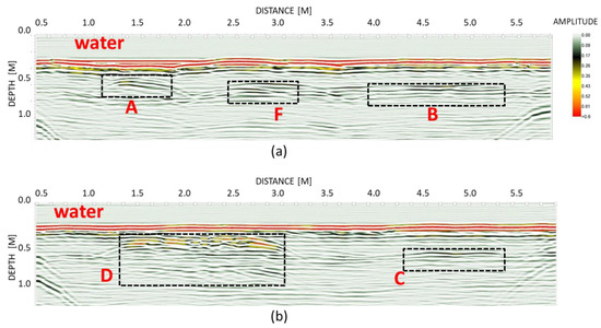
Figure 13.
2D radargrams obtained along the S1 (a) and S2 (b) profiles in Figure 5 with indication of the anomalies related to the archaeological structures.
Even with the presence of water-saturated soil and the water column, the reflections imputable to the column (A), the stone wall (D), and the top of the two tombs (F and D) are clearly individuated (Figure 13a,b) while the top of the road (C) is weakly identifiable.
Moreover, 2D ERTs results are shown in Figure 14. Electrical resistivity measurements were performed with a dipole–dipole array and an electrode spacing of about 0.20 m. Inversions with ResIPy software converged into four iterations reaching the final RMS Misfit of 1.0. The electrical resistivity values range is between 10 and 100 Ωm. In general, the lower resistivity values (<50 Ωm) are due to the presence of the saturated sand while the higher values (>50 Ωm) are induced by the presence of the archaeological remains.
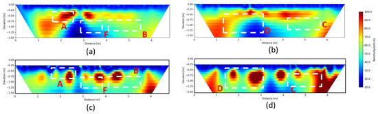
Figure 14.
2D ERTs obtained on S1 and S2 with floating (a,b) and underwater (c,d) electrodes using the dipole–dipole Array (the inversions are performed with ResIPy).
The 2D ERTs were acquired with two different approaches. The electrical resistivity distribution obtained with floating electrodes was not able to detect anomalies well that were associated with the buried objects (Figure 14a,b). It is possible to identify the shallowest features (column A, the wall D) whilst, the features at greater depth, as in the case of the paved road and tombs, are not visible. On the contrary, the electrical resistivity image obtained with electrodes placed on the underwater floor provides an improvement of the information about the position of the archaeological remains (Figure 14c,d). In fact, the shallowest (column A, the wall D) and deeper (paved road and tombs) features are highlighted well.
5. Discussion
Electrical DC and electromagnetic (GPR) techniques were applied to an archaeological framework reconstructed in a laboratory to test the capability of geophysics to identify some objects characterized by different materials (stone, bricks, mortar, etc.) and shapes (rectangular, circular, irregular, etc.) placed in lacustrine and very wet scenarios.
The aim of the experiments was to analyze the limits of the geophysical techniques, as GPR and ERT, when the archaeological structures are below the water level or close to the water table (high water content). The experiment was realized in two distinct phases: in the first one (WP1), ERT and GPR analyses were performed in different scenarios characterized by an increasing water content (WL1–WL2–WL3). The surveys were carried out adopting 3D GPR and ERT. The results have demonstrated the limits of the two methodologies for archaeological issues when the remains are below the water table (high saturation degree).
Regarding GPR surveys, in all the analyzed cases, the influence of the water on the propagation of the em pulses was evident. In Figure 15, the results obtained at the frequency of 400 MHz in the three different scenarios analyzed in WP1 are compared. A strong decay of the radar amplitude signals with the increasing of the groundwater level is clearly recorded.
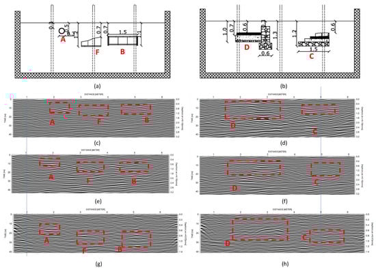
Figure 15.
Comparison of the radargrams acquired in correspondence of the S1 (a) and S2 (b) that represent the main sections of the test site (c). The radargrams acquired in WL3 (c,d), WL2 (e,f), and WL1 (g,h) allow to detect the different structures (anomalies in red).
Further in the first two cases (WL2 and WL3), characterized by a lower water content in the vadose zone, the electromagnetic reflections allow to identify all the buried structures (Figure 15c–f) while in the full saturated case, the GPR anomalies are less evident (15g–h). Figure 16 shows the frequency spectrum of the mean trace for the radargram acquired above the wall and road (S2). In WL2 and WL3 (Figure 16a,b) the signal spectra are almost identical with a limited downshift for the wetter case (Figure 16b). On the contrary, the spectrum in WL1 (Figure 16c) suffers a substantial variation towards the lower frequency where the biggest variation is evident, and the archaeological structures presents are more difficulty to be identified. The frequency centroids estimated for the three cases were equals to 484 MHz (WL3), 406 MHz (WL2) and 348 (WL1) in agreement with the expected signal attenuation in a lossy medium which is affected by absorption and dispersion phenomena able to cause a decay of their amplitude [100].
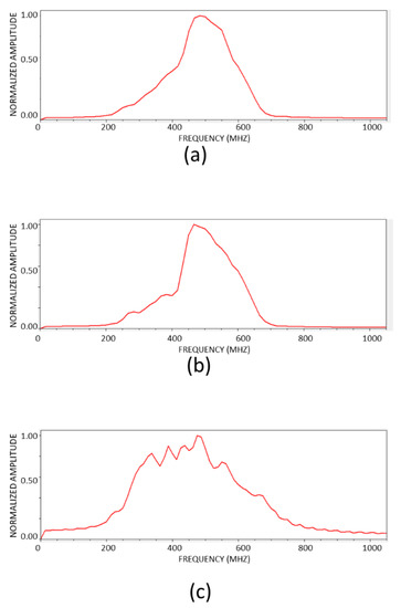
Figure 16.
Frequency spectra of the mean trace related to the radargram acquired in S2 for WL3 (a), WL2 (b), and WL1 (c).
However, the 3D reconstructions obtained with the GPR data have demonstrated a great capability to identify all the structures in WL2 and WL3; in WL1, where the attenuation is greater, it was impossible to detect those objects placed at the greater depths or not perpendicular to the adopted acquisition grid. It is worth noting that some difficulties are also encountered with the drier scenario (WL3) where the results are noisier because the inadequate compaction of the soil and the scarce permittivity contrast did not allow to reconstruct the real shape of the archaeological structure, that are better focused in WL2 where the water content is higher; therefore, the expected geophysical contrast is higher.
In WP2 (underwater scenario), GPR showed encouraging results in presence of non-ionic solutions giving optimal information about the distribution and geometrical shape of the structures despite the attenuation limits (strong variation of the spectrum frequency characterized by a centroid value of 287 MHz). Thus, GPR confirmed its usefulness for the archaeological research also in lacustrine contexts as support of the well-established sound acoustic techniques allowing to obtain a higher resolution.
Results obtained with the 3D ERTs show how important it is to define the best electrode setting; therefore, the simulated approaches in full-scale laboratory experiments help to evaluate the best solution for each kind of detection aims. In our experiments, the results highlight the capability of the loop–loop array to detect the structures buried in the subsoil is greater than the classical dipolar approach. Therefore, these results show the potentiality of this approach for the investigation in areas where obstacles can reduce the possibility to perform electrical analyses with 2D and 3D ERTs based on conventional approaches.
Moreover, 2D ERTs acquired with electrodes located on the water surface show that the high conductive environment and the depth of investigation of the methodology do not allow to easily identify the buried structures. On the contrary, the use of floor embedded electrodes allows to improve the depth of investigation for supporting the detection of the buried structures. Therefore, 2D ERTs can be a suitable contribution for the shallower structures, but the limitations mainly related to the problem of resolution at depth require further efforts to apply in contexts similar to the analyzed ones.
In order to overcome the limits of the single methodology used, the best approach is the integration of electrical resistivity and GPR data. In detail, through a simplified geophysical integration of the GPR and ERT 3D data, based on the model co-rendered image process [101], the integration of the methodologies provides good information for the localization of the archaeological buried remains as shown in Figure 17. 3D ERTs have provided acceptable results only in the drier conditions (WL2 and WL3). The cause is due to the low resolution of the method when the water table was shallower (WL1) and the electrical contrasts were weak. However, the strong reflections are generally correspondent to the higher electrical anomalies, and where one of the two methodology struggles, the other one can support the detection of the structure. This is the case of the capuchin tomb (F), which is not clearly detectable by the GPR data due to its orientation with respect to the acquisition direction, whereas ERT data clearly identify the presence of a strong electrical anomaly where the tomb is expected. On the contrary, the rectangular tomb (B) is well detectable with the GPR, while it is not visible for the ERT because its position too marginal within the acquisition scheme.
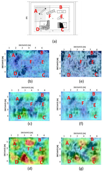
Figure 17.
Model co-rendered GPR and ERT loop–loop depth slices at 0.45 m (left column) and 0.70 m (right column) in WL1 (b–e), WL2 (c–f), and WL3 (d–g) with the site plan (a).
Moreover, GPR radargrams and ERTs acquired along S1 and S2 during WP2 (underwater conditions) are model co-rendered and the results are plotted in Figure 18. The first level of integration highlights the capability of both the methods to detect electric and em anomalies in correspondence of the buried structures despite the different resolution. Generally, the presence of strong reflections implies anomalies of the electrical behaviour of the subsoil related to the presence of archaeological remains. The results are in good agreement, especially in the upper layer where the ERTs, acquired with the electrodes fixed into the floor, have the better resolution and all the structures are distinguishable.
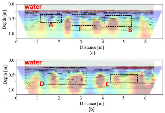
Figure 18.
Model co-rendered GPR and ERT data acquired along the two main sections (a,b) in WP2.
A further quantitative consideration can be realized comparing the geophysical detected anomalies both with the GPR and the ERTs with the real sizes and depths of the various objects buried in the subsoil. As previously shown, the used geophysical methods were able to detect the buried structures and the GPR was the best one in the different scenarios. In Figure 19 and Figure 20, a preliminary quantitative analysis between the geophysical and expected results in the plan is shown in terms of position and size of the detected structures, which reveal the greater or lesser capability of the used methodology for the localization and characterization of the archaeological features for the different water levels adopted in WP1 where 3D acquisitions were performed. It is evident how in wetter conditions GPR is more able for detecting the real sizes of the elements. This is clearly due to the reflection focusing effects induced by the increase of the dielectric permittivity related to the background soil. GPR results further highlight a wrong positioning of the column if compared with the planned design. The best results are obtained for those elements with regular shape, as in the cases of the rectangular tomb, paved road, and stone wall. In detail, as showed in Figure 19, the anomaly of the column in WL2 is equal to the expected sizes of 1.4 m × 0.2 m; the reflections related to the rectangular tomb in WL1 highlight an anomaly really similar to the real one; similarly, the anomalies recorded in WL2 and WL1 for the stone wall with sizes of 1.6 m × 1.6 m. Further, there is a strong agreement between the reflections induced by the paved road and its planimetric development. Regarding the enchytrismos, only in WL1 were the detected sizes adequately matched with the real ones. The depth of the objects, when detected, generally complies with the real ones, and some discrepancies can be related to the heterogenous compaction degree of the sand placed above the structures.
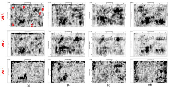
Figure 19.
Comparison of GPR slices at the depths of 0.25 m (a), 0.45 m (b), 0.70 m (c) and 1.00 m (d) for the different scenarios in WP1.
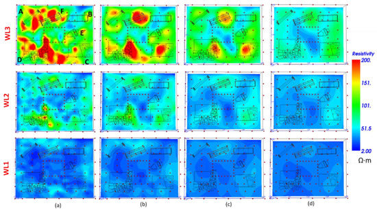
Figure 20.
Comparison of ERT slices at the depths of 0.25 m (a), 0.45 m (b), 0.70 m (c) and 1.00 m (d) for the different scenarios in WP1.
Despite the lower resolution, ERTs have detected some archaeological structures and in the case of the paved road and stone wall, have permitted to characterize the sizes with high detail. This is particularly true for WL2 when the water saturation degree is in intermediate conditions. Regarding the other buried objects, it is possible to define only the position; indeed, the sizes of the resulting electrical anomalies do not allow to reconstruct the expected geometries.
As summarized in Table 3, GPR has permitted to quantitatively characterize, with high accuracy, the sizes of the buried objects when the strong geophysical contrast occurs as in the case of WL1, while the lower attenuation of WL2 and WL3 makes the identification of the structures more difficult. Regarding ERT, the higher water content of WL1 do not allow to reconstruct the real shape of the buried objects, while in WL2 and WL3, the results are encouraging for real application in the archaeological field.
Table 3.
Comparison between the expected and geophysical results for the detection of the buried object in terms of position and size for WL1, WL2, and WL3 in WP1.
6. Conclusions
The geophysical tests realized at the Hydrogeosite laboratory for testing the capability of ERT and GPR for archaeological purposes in humid and lacustrine scenarios have provided interesting results. In particular, GPR measurements constituted a valid support in humid/lacustrine scenarios, but their usefulness depends strongly on the size and positions of the buried structures as demonstrated in WP1. Furthermore, as shown in WP2, GPR can work very well, both near the banks of rivers and lakes and above the water providing an excellent resolution; however, a crucial role is played in this case by the required investigation depth.
The applicability of ERT needs more attention; in particular, the resolution and quality of the electrode contacts should be considered carefully in order to obtain results acceptable from the archaeological point of view. The best results in this work were achieved with analyses carried out with the 3D loop–loop array; whilst the use of the classical 3D array with electrodes equispaced in two directions did not allow to easily localize the archaeological features. This result is very interesting for the applicability of the resistivity methods often not used in urban scenarios where regular disposition of the electrodes are not always fully achievable for the constant presence of obstacle (trees, monuments, urban furniture, etc.). In WP2, the 2D ERT profiles have highlighted the capability of the methodology to identify strong anomalies in correspondence of the shallower structures showing the usefulness of the resistivity methods in very conductive scenarios.
Despite great efforts carried out for the test, some limitations are difficult to overcome; therefore, a qualitative integration of GPR and ERT data was tried by co-rendering the images. In this research, the integration was effectively created by adopting 3D and 2D data for the WP1 and WP2, respectively, and the results obtained demonstrate, unequivocally, the importance of the comparison and integration of different methodologies for improving the localization and identification of the buried structures in humid and wetland scenarios.
In the future, greater efforts will be required to integrate the geophysical data aimed at obtaining quantitative information about the planimetric and volumetric structures placed in the subsoil also involving the use of advanced adopting algorithms (i.e., image data-fusion, machine learning algorithms). At the same time, a further topic of the GPR research analyses will be to identify the best strategies for the migration of the hyperbola in order to make quantitative analyses possible.
Author Contributions
Conceptualization, E.R., F.P. and L.C.; methodology, L.C., V.G. and E.R.; investigation, L.C., F.P., G.D.M., V.G. and E.R.; data processing, L.C., V.G. and E.R.; technical supervision, G.D.M.; writing—original draft preparation, L.C.; writing—review and editing, E.R., L.C. and V.G.; visualization, L.C., E.R. and V.G.; project administration, E.R. and V.L.; final review, E.R. and V.L. All authors have read and agreed to the published version of the manuscript.
Funding
The experiments are funded by the Basilicata Region, Progetto PO FSE Basilicata 2007–2013: “Promozione della ricerca e dell’innovazione e sviluppo di relazioni con il sistema produttivo regionale” DD n. 796/2013 Azione n. n. 15/AP/05/2013/REG.
Institutional Review Board Statement
Not applicable.
Informed Consent Statement
Not applicable.
Data Availability Statement
The data that support the findings of this study are available from the corresponding author upon reasonable request.
Acknowledgments
The experiments were funded by the Basilicata Region, Progetto PO FSE Basilicata 2007–2013: “Promozione della ricerca e dell’innovazione e sviluppo di relazioni con il sistema produttivo regionale” DD n. 796/2013 Azione n. n. 15/AP/05/2013/REG. We are grateful to the Director of the CNR Institute of Methodologies for Environmental Analysis for the experimental phase in the Laboratory Hydrogeosite facility.
Conflicts of Interest
The authors declare no conflict of interest.
References
- Rizzo, E.; Chianese, D.; Lapenna, V. Integration of magnetometric, GPR and geoelectric measurements applied to the archaeological site of Viggiano (Southern Italy, Agri Valley-Basilicata). Near Surf. Geophys. 2005, 3, 13–19. [Google Scholar] [CrossRef]
- Campana, S.; Dabas, M.; Marasco, L.; Piro, S.; Zamuner, D. Integration of remote sensing, geophysical surveys and arcaheological excavations for the study of a medieval mound (Tuscany, Italy). Archaeol. Prospect. 2009, 16, 167–176. [Google Scholar] [CrossRef]
- Piro, S.; Ceraudo, G.; Zamuner, D. Integrated Geophysical and Archaeological Investigations of Aquinum in Frosinone, Italy. Archaeol. Prospect. 2011, 18, 127–138. [Google Scholar] [CrossRef]
- Filzwieser, R.; Olesen, L.H.; Neubauer, W. Large-scale geophysical archaeological prospection pilot study at Viking Age and medieval sites in west Jutland, Denmark. Archaeol. Prospect. 2017, 24, 373–393. [Google Scholar] [CrossRef]
- Tsokas, G.N.; Tsourlos, P.I.; Kim, J.-H.; Papazachos, C.B.; Vargemezis, G.; Bogiatzis, P. Assessing the Condition of the Rock Mass over the Tunnel of Eupalinus in Samos (Greece) using both Conventional Geophysical Methods and Surface to Tunnel Electrical Resistivity Tomography. Archaeol. Prospect. 2014, 21, 277–291. [Google Scholar] [CrossRef]
- Leucci, G.; Parise, M.; Sammarco, M.; Scardozzi, G. The Use of Geophysical Prospections to Map Ancient Hydraulic Works: The Triglio Underground Aqueduct (Apulia, Southern Italy). Archaeol. Prospect. 2016, 23, 195–211. [Google Scholar] [CrossRef]
- Capozzoli, L.; Catapano, I.; De Martino, G.; Gennarelli, G.; Ludeno, G.; Rizzo, E.; Soldovieri, F.; Uliano Scelza, F.; Zuchtriegel, G. The Discovery of a Buried Temple in Paestum: The Advantages of the Geophysical Multi-Sensor Application. Remote Sens. 2020, 12, 2711. [Google Scholar] [CrossRef]
- Binley, A.; Hubbard, S.S.; Huisman, J.A.; Revil, A.; Robinson, D.A.; Singha, K.; Slater, L.D. The emergence of hydrogeophysics for improved understanding of subsurface processes over multiple scales. Water Resour. Res. 2015, 51, 3837–3866. [Google Scholar] [CrossRef]
- Bowens, A. Underwater Archaeology—The NAS Guide to Principles and Practice, 2nd ed.; Nautical Archaeological Society: Wales, UK, 2012; ISBN 978-1-405-17592-0. [Google Scholar]
- Winton, T. Quantifying Depth of Burial and Composition of Shallow Burie Archaeological Material: Integrated Sub-bottom Profiling and 3D Survey Approaches. In 3D Recording and Interpretation for Maritime Archaeology; Mc Carthy, J.K., Benjamin, J., Winton, T., van Duivenvoorde, W., Eds.; Springer: New York, NY, USA, 2019. [Google Scholar]
- Westley, K.; Mcneary, R. Archaeological Applications of Low-Cost Integrated Sidescan Sonar/Single-Beam Echosounder Systems in Irish Inland Waterways. Archaeol. Prospect. 2017, 24, 37–57. [Google Scholar] [CrossRef]
- Tizzard, L.; Bicket, A.R.; Benjamin, J.; Loecker, D.D. A Middle Palaeolithic site in the southern North Sea: Investigating the archaeology and palaeogeography of Area 240. J. Quat. Sci. 2014, 29, 698–710. [Google Scholar] [CrossRef]
- Zielhofer, C.; Rabbel, W.; Wunderlich, T.; Vött, A.; Berg, S. Integrated geophysical and (geo)archaeological explorations in wetlands. Quat. Int. 2018, 473, 1–2. [Google Scholar] [CrossRef]
- Abramov, A.; Vasiliev, A. Underwater ground penetrating radar in archeological investigation below sea bottom. In Proceedings of the Tenth International Conference on Grounds Penetrating Radar, Delft, The Netherlands, 21–24 June 2004; IEEE: Piscataway, NJ, USA, 2004; pp. 455–458. [Google Scholar]
- Ruffell, A. Under-water scene investigation using ground penetrating radar (GPR) in the search for a sunken jet ski, Northern Ireland. Sci. Justice 2006, 46, 221–230. [Google Scholar] [CrossRef]
- Yang, C.H.; Tong, L.T.; Yu, C.Y. Integrating GPR and RIP methods for water surface detection of geological structures. Terr. Atmos. Ocean. Sci. 2006, 17, 391–404. [Google Scholar] [CrossRef]
- Qin, T.; Zhao, Y.; Lin, G.; Hu, S.; An, C.; Geng, D.; Rao, C. Underwater archaeological investigation using ground penetrating radar: A case analysis of Shanglinhu Yue Kiln sites (China). J. Appl. Geophys. 2018, 154, 11–19. [Google Scholar] [CrossRef]
- Ruffell, A.; Parker, R. Water penetrating radar. J. Hydrol. 2021, 597, 126300. [Google Scholar] [CrossRef]
- Giampaolo, V.; Capozzoli, L.; Grimaldi, S.; Rizzo, E. Sinkhole risk assessment by ERT: The case study of Sirino Lake (Basilicata, Italy). Geomorphology 2016, 253, 1–9. [Google Scholar] [CrossRef]
- Dahlin, T.; Loke, M.H. Underwater ERT surveying in water with resistivity layering with example of application to site investigation for a rock tunnel in central Stockholm. Near Surf. Geophys. 2018, 16, 230–237. [Google Scholar] [CrossRef]
- Simyrdanis, K.; Bailey, M.; Moffat, I.; Roberts, A.; van Duivenvoorde, W.; Savvidis, A.; Cantoro, G.; Bennett, K.; Kowlessar, J. Resolving Dimensions: A Comparison Between ERT Imaging and 3D Modelling of the Barge Crowie, South Australia. In 3D Recording and Interpretation for Maritime Archaeology; Mc Carthy, J.K., Ed.; Springer: New York, NY, USA, 2019. [Google Scholar]
- Papadopoulos, N.; Oikonomou, D.; Simyrdanis, K.; Heng, L.M. Practical considerations for shallow submerged archaeological prospection with 3-D electrical resistivity tomography. Archaeol. Prospect. 2021, 28, 1–21. [Google Scholar] [CrossRef]
- De Souza, H.; Sampaio, E.E.S. Apparent resistivity and spectral induced polarization in the submarine environment. An. Acad. Bras. Cienc. 2001, 73, 429–444. [Google Scholar] [CrossRef]
- Kwon, H.; Kim, J.; Ahn, H.; Yoon, J.; Kim, K.; Jung, C.; Lee, S.; Uchida, T. Delineation of fault zone beneath a riverbed by an electrical resistivity survey using a floating stream cable. Explor. Geophys. 2005, 36, 50–58. [Google Scholar] [CrossRef]
- Freyer, P.A.; Nyquist, J.E.; Toran, L.E. Use of underwater resistivity in the assessment of groundwater–surface water interaction within the burd run watershed. In Proceedings of the Annual Symposium on the Application of Geophysics to Engineering and Environmental Problems 8; Environmental and Engineering Geophysical Society: Seattle, WA, USA, 2006. [Google Scholar]
- Losito, G.; Aminti, P.L.; Martelletti, L.; Grandjean, J.-M.; Mazzetti, A.; Trova, A.; Benvenuti, G. Marine geoelectrical prospecting for soft structures characterization in shallow water: Field and laboratory test. In Proceedings of the EAGE 69th Conference & Exhibition, London, UK, 11–14 June 2007; European Association of Geoscientists & Engineers: Houten, The Netherlands, 2007. [Google Scholar]
- Crook, N.; Binley, A.; Knight, R.; Robinson, D.A.; Zarnetske, J.; Haggerty, R. Electrical resistivity imaging of the architecture of substream sediments. Water Resour. Res. 2008, 44, W00D13. [Google Scholar] [CrossRef]
- Nyquist, J.E.; Freyer, P.A.; Toran, L. Stream bottom resistivity tomography to map ground water discharge. Ground Water 2008, 46, 561–569. [Google Scholar] [CrossRef] [PubMed]
- Henderson, R.D.; Day-Lewis, F.D.; Abarca, E.; Harvey, C.F.; Karam, H.N.; Liu, L.; Lane, J.W. Marine electrical resistivity imaging of submarine groundwater discharge: Sensitivity analysis and application in Waquoit Bay, Massachusetts, USA. Hydrogeol. J. 2010, 18, 173–185. [Google Scholar] [CrossRef]
- Day-Lewis, F.D.; White, E.A.; Johnson, C.D.; Lane, J.W.J.R.; Belaval, M. Continuous resistivity profiling to delineate submarine groundwater discharge—Examples and limitations. Lead. Edge 2006, 25, 724–728. [Google Scholar] [CrossRef]
- Castilho, G.; Maia, D. A successful mixed land underwater 3D resistivity survey in an extremely challenging environment in Amazônia. In Proceedings of the 21st EEGS Symposium on the Application of Geophysics to Engineering and Environmental Problems, Philadelphia, PA, USA, 6–10 April 2008; Environmental and Engineering Geophysical Society (EEGS): Denver, CO, USA, 2008; pp. 1150–1158. [Google Scholar]
- Baumgartner, F. A new method for geoelectrical investigations underwater. Geophys. Prospect. 1996, 44, 71–98. [Google Scholar] [CrossRef]
- Mansoor, N.; Slater, L. Aquatic electrical resistivity imaging of shallow-water wetlands. Geophysics 2007, 72, F211–F221. [Google Scholar] [CrossRef]
- Loke, M.H.; Lane, J.W., Jr. Inversion of Data from Electrical Resistivity Imaging Surveys in Water-Covered Areas. Explor. Geophys. 2004, 35, 266–271. [Google Scholar] [CrossRef]
- Rizzo, E.; Straface, S.; Chidichimo, S.; Votta, M.; Lapenna, V. First hydrogeophysical controlled experiments in the large lab-scale Hydrogeosite Laboratory (IMAA-CNR). Geophys. Res. Abstr. 2008, 10, 9492. [Google Scholar]
- Capozzoli, L.; Caputi, A.; De Martino, G.; Giampaolo, V.; Luongo, R.; Perciante, F.; Rizzo, E. Electrical and electromagnetic techniques applied to an archaeological framework reconstructed in laboratory. In Advanced Ground Penetrating Radar (IWAGPR), Proceedings of the 2015 8th International Workshop on Advanced Ground Penetrating Radar, Firenze, Italy, 7–10 July 2015; IEEE: Piscataway, NJ, USA, 2015. [Google Scholar]
- Capozzoli, L.; De Martino, G.; Giampaolo, V.; Perciante, F.; Rizzo, E. Geophysical techniques applied to investigate underwater structures. In Advanced Ground Penetrating Radar (IWAGPR), Proceedings of the 2017 9th International Workshop on Advanced Ground Penetrating Radar, Edimbourgh, Scotland, 28–30 June 2017; IEEE: Piscataway, NJ, USA, 2017. [Google Scholar]
- Ludeno, G.; Capozzoli, L.; Rizzo, E.; Soldovieri, F.; Catapano, I. A Microwave Tomography Strategy for Underwater Imaging via Ground Penetrating Radar. Remote Sens. 2018, 10, 1410. [Google Scholar] [CrossRef]
- Rizzo, E.; Capozzoli, L. Integrated Geophysical Techniques for Archaeological Remains: Real Cases and Full Scale Laboratory Example. In Archaeogeophysics; El-Qady, G., Metwaly, M., Eds.; Springer International Publishing AG, Part of Springer Nature: New York, NY, USA, 2019; Chapter 13. [Google Scholar] [CrossRef]
- Goodman, D.; Piro, S. GPR Remote Sensing in Archaeology; Springer: London, UK, 2013. [Google Scholar]
- Daniels, D.J. Ground Penetrating Radar, 2nd ed.; The Institute of Electrical Engineers: London, UK, 2004. [Google Scholar]
- Davis, J.L.; Annan, A.P. Ground penetrating radar for high-resolution mapping of soil and rock stratigraphy. Geophys. Prospect. 1989, 37, 531–551. [Google Scholar] [CrossRef]
- Doolittle, J.A.; Collins, M.E. Use of soil information to determine application of ground-penetrating radar. J. Appl. Geophys. 1995, 33, 101–108. [Google Scholar] [CrossRef]
- Walther, E.G.; Pitchford, A.M.; Olhoeft, G.R. A strategy for detecting subsurface organic contaminants. In The Petroleum Hydrocarbons and Organic Chemicals in Ground Water, Prevention, Detection and Restoration; National Water Well Association: Houston, TX, USA, 1986; pp. 357–381. [Google Scholar]
- Capozzoli, L.; Mutino, S.; Liseno, M.G.; De Martino, G. Searching for the History of the Ancient Basilicata: Archaeogeophysics Applied to the Roman Site of Forentum. Heritage 2019, 2, 1097–1116. [Google Scholar] [CrossRef]
- Vickers, R.S.; Dolphin, L.T. A communication on an archaeological radar experiment at Chaco Canyon, New Mexico. MASCA Newslett. 1975, 11, 6–8. [Google Scholar]
- Nishimura, Y.; Goodman, D. Ground penetrating radar survey at Wroxeter. Archaeol. Prospect. 2000, 7, 101–105. [Google Scholar] [CrossRef]
- Neubauer, W.; Eder-Hinterleitner, A.; Seren, S.; Melichar, P. Georadar in the Roman civil town Carnuntum, Austria: An approach for archaeological interpretation of GPR data. Archaeol. Prospect. 2002, 9, 135–156. [Google Scholar] [CrossRef]
- Conyers, L.B.; Ernenwein, E.G.; Bedal, L.A. Ground-penetrating radar discovery at Petra, Jordan. Antiquity 2009, 76, 339–340. [Google Scholar] [CrossRef]
- Gaffney, V.; Patterson, H.; Piro, S.; Goodman, D.; Nishimura, Y. Multimethodological approach to study and characterise Forum Novum (Vescovio, Central Italy). Archaeol. Prospect. 2004, 11, 201–212. [Google Scholar] [CrossRef]
- Piro, S.; Goodman, D.; Nishimura, Y. The study and characterization of Emperor Traiano’s villa using high-resolution integrated geophysical surveys. Archaeol. Prospect. 2003, 10, 1–25. [Google Scholar] [CrossRef]
- Chianese, D.; D’Emilio, M.; Di Salvia, S.; Lapenna, V.; Ragosta, M.; Rizzo, E. Magnetic Mapping, Ground Penetrating Radar Surveys and Magnetic Susceptibility Measurements for the Study of the Archaeological Site of Serra di Vaglio (Southern Italy). J. Archaeol. Sci. 2004, 31, 633–643. [Google Scholar] [CrossRef]
- Goodman, D.; Piro, S.; Nishimura, Y.; Patterson, H.; Gaffney, V. Discovery of a 1st century AD Roman amphitheater and other structures at the Forum Novum by GPR. J. Environ. Eng. Geophys. 2004, 9, 35–41. [Google Scholar] [CrossRef]
- Seren, S.; Eder-Hinterleitner, A.; Neubauer, W.; Löcker, K.; Melichar, P. Extended comparison of different GPR systems and antenna configurations at the Roman site Carnuntum. Near Surf Geophys. 2007, 5, 389–394. [Google Scholar] [CrossRef]
- Campana, S.; Piro, S. Seeing the Unseen—Geophysics and Landscape Archaeology; CRC Press: London, UK, 2009; Volume 2, 376p, ISBN 978-0-415-44721-8. [Google Scholar]
- Novo, A.; Sala, R.; Garcìa, E.; Tamba, R.; Muñoz, F.; Solla, M.; Lorenzo, H. From Celtiberians to Romans: Combined geophysical (3D GPR and fluxgate gradiometer) prospection for the archaeological characterization of Castro de la Magdalena (Leon, Spain). ArchaeoSciences 2009, 33, 121–124. [Google Scholar] [CrossRef]
- Grasmueck, M.; Weger, R.; Horstmeyer, H. Three-dimensional ground-penetrating radar imaging of sedimentary structures, fractures, and archaeological features at submeter resolution. Geology 2004, 32, 933–936. [Google Scholar] [CrossRef]
- Grasmueck, M.; Weger, R.; Horstmeyer, H. Full-resolution 3D imaging. Geophysics 2005, 70, 12–19. [Google Scholar] [CrossRef]
- Annan, P. Electromagnetic principles of ground penetrating radar. In Ground Penetrating Radar: Theory and Applications; Jol, H.M., Ed.; Elsevier: Amsterdam, The Netherlands, 2009; pp. 1–40. ISBN 978-0-444-53348-7. [Google Scholar]
- Bavusi, M.; Giocoli, A.; Rizzo, E.; Lapenna, V. Geophysical characterisation of Carlo’s V Castle (Crotone, Italy). J. Appl. Geophys. 2009, 67, 386–401. [Google Scholar] [CrossRef]
- Rizzo, E.; Masini, N.; Lasaponara, R.; Orefici, G. ArchaeoGeophysical methods in the Templo del Escalonado (Cahuachi, Nasca, Perù). Near Surf. Geophys. 2010, 8, 433–439. [Google Scholar] [CrossRef]
- Rizzo, E.; Santoriello, A.; Capozzoli, L.; De Martino, G.; De Vita, C.B.; Musmeci, D.; Perciante, F. Geophysical survey and archaeological data at Masseria Grasso (BN, Italy). Surv. Geophys. 2018, 39, 1201–1217. [Google Scholar] [CrossRef]
- Zhao, W.; Tian, G.; Forte, E.; Pipan, M.; Wang, Y.; Li, X.; Shi, Z.; Liu, H. Advances in GPR data acquisition and analysis for archaeology. Geophys. J. Int. 2015, 202, 62–71. [Google Scholar] [CrossRef]
- Binley, A.; Kemna, A. DC resistivity and induced polarization methods. In Hydrogeophysics; Rubin, Y., Hubbard, S.S., Eds.; (Water Science and Technology Library Ser. 50); Springer: New York, NY, USA, 2005; pp. 129–156. [Google Scholar]
- Chang, P.Y.; Chang, S.K.; Liu, H.C.; Wang, S.C. Using integrated 2D and 3D resistivity imaging methods for illustrating the mud-fluid conduits of the Wushanting mud volcanoes in southwestern Taiwan. Terr. Atmos. Ocean. Sci. 2011, 22, 1–14. [Google Scholar] [CrossRef]
- Loke, M.H.; Barker, R.D. Practical techniques for 3D resistivity surveys and data inversion. Geophys. Prosp. 1996, 44, 499–523. [Google Scholar] [CrossRef]
- DeGroot-Hedlin, C.; Constable, S. Occams’ inversion to generate smooth, two-dimensional models from magnetotelluric data. Geophysics 1990, 55, 1613–1624. [Google Scholar] [CrossRef]
- Noel, M.; Xu, B. Archaeological investigation by electrical resistivity tomography: A preliminary study. Geophys. J. Int. 1991, 107, 95–102. [Google Scholar] [CrossRef]
- Tsokas, G.N.; Giannopoulos, A.; Tsourlos, P.; Vargemezis, G.; Tealby, J.M.; Sarris, A.; Papazachos, C.B.; Savopoulou, T. A large scale geophysical survey in the archaeological site of Europos (northern Greece). J. Appl. Geophys. 1994, 32, 85–98. [Google Scholar] [CrossRef]
- Piro, S.; Tsourlos, P.; Tsokas, G.N. Cavity detection employing advanced geophysical techniques: A case study. Eur. J. Environ. Eng. Geophys. 2001, 6, 3–31. [Google Scholar]
- Drahor, M.G.; Berge, M.A.; Kurtulmus, T.O.; Hartmann, M.; Speidel, M.A. Magnetic and Electrical Resistivity Tomography Investigations in a Roman Legionary Camp Site (Legio IV Scythica) in Zeugma, Southeastern Anatolia, Turkey. Archaeol. Prospect. 2008, 15, 159–186. [Google Scholar] [CrossRef]
- Cardarelli, E.; Fishanger, F.; Piro, S. Integrated geophysical survey to detect buried structures for archaeological prospecting. A case-history at Sabine Necropolis (Rome—Italy). Near Surf. Geophys. 2007, 6, 15–20. [Google Scholar] [CrossRef]
- Elwaseif, M.; Slater, L. Quantifying tomb geometries in resistivity images using watershed algorithms. J. Archaeol. Sci. 2010, 37, 1424–1436. [Google Scholar] [CrossRef]
- Passaro, S. Marine electrical resistivity tomography for shipwreck detection in very shallow water: A case study from Agropoli (Salerno, Southern Italy). J. Archaeol. Sci. 2010, 37, 1989–1998. [Google Scholar] [CrossRef]
- Trogu, A.; Ranieri, G.; Calcina, S.; Piroddi, L. The Ancient Roman Aqueduct of Karales (Cagliari, Sardinia, Italy): Applicability of Geophysics Methods to Finding the Underground Remains. Archaeol. Prospect. 2014, 3, 157–168. [Google Scholar] [CrossRef]
- Tonkov, N.; Loke, M.H. A resistivity survey of a burial mound in the Valley of the Thracian Kings’. Archaeol. Prospect. 2006, 13, 129–136. [Google Scholar] [CrossRef]
- Astin, T.; Eckardt, H.; Hay, S. Resistivity imaging survey of the Roman barrows at Bartlow, Cambridgeshire, UK. Archaeol. Prospect. 2007, 14, 24–37. [Google Scholar] [CrossRef]
- Chianese, D.; Lapenna, V.; Di Salvia, S.; Perrone, A.; Rizzo, E. Joint geophysical measurements to investigate the rossano of Vaglio archaeological site (Basilicata Region, Southern Italy). J. Archaeol. Sci. 2010, 37, 2237–2244. [Google Scholar] [CrossRef]
- Espino, D.; Tejero-Andrade, A.; Cifuentes-Nava, G.; Iriarte, L.; Farías, S.; Chávez, R.E.; López, F. 3D electrical prospection in the archaeological site El Pahñu, Hidalgo State, Central Mexico. J. Archaeol. Sci. 2013, 40, 1213–1223. [Google Scholar] [CrossRef]
- Tsourlos, P.; Papadopoulos, N.; Papazachos, C.; Yi, M.-J.; Kim, J.-H. Efficient 2D inversion of long ERT sections. J. Appl. Geophys. 2014, 105, 213–224. [Google Scholar] [CrossRef]
- Capizzi, P.; Cosentino, P.L.; Fiandaca, G.; Martorana, R.; Messina, P.; Vassallo, S. Geophysical investigations in the archaeological site of Himera (Northern Sicily). Near Surf. Geophys. 2007, 5, 417–426. [Google Scholar] [CrossRef]
- Negri, S.; Leucci, G.; Mazzone, F. High resolution 3D ERT to help GPR data interpretation for researching archaeological items in a geologically complex subsurface. J. Appl. Geophys. 2008, 65, 111–120. [Google Scholar] [CrossRef]
- Keay, S.; Earl, G.; Hay, S.; Kay, S.; Ogden, J.; Strutt, K.D. The role of integrated geophysical survey methods in the assessment of archaeological landscapes: The case of Portus. Archaeol. Prospect. 2009, 16, 154–166. [Google Scholar] [CrossRef]
- Orlando, L. GPR to constrain ERT data inversion in cavity searching: Theoretical and practical applications in archeology. J. Appl. Geophys. 2013, 89, 35–47. [Google Scholar] [CrossRef]
- Jiang, A.; Chen, F.; Masini, N.; Capozzoli, L.; Romano, G.; Sileo, M.; Yang, R.; Tang, P.; Chen, P.; Lasaponara, R. Archaeological crop marks identified from Cosmo-SkyMed time series: The case of Han-Wei capital city, Luoyang, China. Int. J. Digit. Earth (TJDE) 2017, 10, 846–860. [Google Scholar] [CrossRef]
- Masini, N.; Capozzoli, L.; Chen, P.; Chen, F.; Romano, G.; Lu, G.; Tang, P.; Sileo, M.; Ge, Q.; Lasaponara, R. Towards an operational use of Remote Sensing in Archaeology in Henan (China): Archaeogeophysical investigations, approach and results in Kaifeng. Remote Sens. 2017, 9, 809. [Google Scholar] [CrossRef]
- Rizzo, E.; Capozzoli, L.; de Martino, G.; Grimaldi, S. Urban Geophysical approach to characterize the subsoil of the main square in San Benedetto del Tronto town (Italy). J. Eng. Geol. 2019, 257, 105133. [Google Scholar] [CrossRef]
- Capozzoli, L.; de Martino, G.; Capozzoli, V.; Duplouy, A.; Henning, A.; Rizzo, E. The pre-Roman hilltop settlement of Monte Torretta di Pietragalla: First results of the geophysical survey. Archaeol. Prospect. 2021, 28, 1–14. [Google Scholar] [CrossRef]
- Giovannoni, G. La Tecnica delle Costruzioni Presso i Romani; Società Editrice di Arte Illustrate: Rome, Italy, 1925. [Google Scholar]
- Lugli, G. La Tecnica Edilizia Romana; Giovanni Bardi: Rome, Italy, 1957. [Google Scholar]
- Adam, J.P. L’arte di Costruire Presso i Romani; Materiale e Tecniche; Longanesi: Milano, Italy, 1998. [Google Scholar]
- Giuliani, C.F.; Ferretti, A.S. Opus cementicium. Il materiale e la tecnica costruttiva, Atti del seminario (Roma, facoltà di Ingegneria, 11/06/1997). In Materie e Strutture; fasc. 2–3; L’Erma di Bretschneider: Rome, Italy, 1997. [Google Scholar]
- Giuffrè, A. Letture sulla Meccanica delle Murature Storiche; Kappa Ed: Rome, Italy, 1999. [Google Scholar]
- Le Pera, S. Come Costruivano Gli Antichi Romani: Brevi Note di Tecnica Edilizia; Palombi Editore: Roma, Italy, 1999. [Google Scholar]
- Caleca, L. Architettura Tecnica; Flaccovio Editore: Palermo, Italy, 2000. [Google Scholar]
- Rocchietti, D. Aree Sepolcrali a Metaponto; Consiglio Regionale della Basilicata: Potenza, Italy, 2002. [Google Scholar]
- Giuliani, C.F. L’edilizia nell’Antichità; Carocci: Rome, Italy, 2006. [Google Scholar]
- Morelli, G.; LaBrecque, D.J. Advances in ERT inverse modelling. Eur. J. Environ. Eng. Geophys. 1996, 1, 171–186. [Google Scholar]
- Blanchy, G.; Saneiyan, S.; Boyd, J.; McLachlan, P.; Binley, A. ResIPy, an intuitive open source software for complex geoelectrical inversion/modeling. Comput. Geosci. 2020, 137, 104423. [Google Scholar] [CrossRef]
- Liu, L.; Lane, J.W.; Quan, Y. Radar attenuation tomography using the centroid frequency downshift method. J. Appl. Geophys. 1998, 40, 105–116. [Google Scholar] [CrossRef]
- Dell’Aversana, P. From rock physics to geophysical data integration: Theory, applications and implications. First Break 2014, 32, 159–161. [Google Scholar] [CrossRef]


Publisher’s Note: MDPI stays neutral with regard to jurisdictional claims in published maps and institutional affiliations. |
© 2022 by the authors. Licensee MDPI, Basel, Switzerland. This article is an open access article distributed under the terms and conditions of the Creative Commons Attribution (CC BY) license (https://creativecommons.org/licenses/by/4.0/).