Article

Modeling and Control of an Articulated Multibody Aircraft

1
UniSA STEM, University of South Australia, Adelaide 5095, Australia
2
Department of Aerospace Engineering, Faculty of Engineering, Universiti Putra Malaysia, Serdang 43400, Malaysia
3
Defence Science and Technology Group, Joint and Operations Analysis Division, Melbourne 3207, Australia
*
Author to whom correspondence should be addressed.
Appl. Sci. 2022, 12(3), 1162; https://doi.org/10.3390/app12031162
Submission received: 10 December 2021 / Revised: 12 January 2022 / Accepted: 19 January 2022 / Published: 23 January 2022
(This article belongs to the Special Issue Dynamic Phenomena)

Abstract

:
Insects use dynamic articulation and actuation of their abdomen and other appendages to augment aerodynamic flight control. These dynamic phenomena in flight serve many purposes, including maintaining balance, enhancing stability, and extending maneuverability. The behaviors have been observed and measured by biologists but have not been well modeled in a flight dynamics framework. Biological appendages are generally comparatively large, actuated in rotation, and serve multiple biological functions. Technological moving masses for flight control have tended to be compact, translational, internally mounted and dedicated to the task. Many flight characteristics of biological flyers far exceed any technological flyers on the same scale. Mathematical tools that support modern control techniques to explore and manage these actuator functions may unlock new opportunities to achieve agility. The compact tensor model of multibody aircraft flight dynamics developed here allows unified dynamic and aerodynamic simulation and control of bioinspired aircraft with wings and any number of idealized appendage masses. The demonstrated aircraft model was a dragonfly-like fixed-wing aircraft. The control effect of the moving abdomen was comparable to the control surfaces, with lateral abdominal motion substituting for an aerodynamic rudder to achieve coordinated turns. Vertical fuselage motion achieved the same effect as an elevator, and included potentially useful transient torque reactions both up and down. The best performance was achieved when both moving masses and control surfaces were employed in the control solution. An aircraft with fuselage actuation combined with conventional control surfaces could be managed with a modern optimal controller designed using the multibody flight dynamics model presented here.

1. Introduction

The potential applications of small unmanned aerial vehicles (SUAVs) for both military and civil applications continue to drive interest in their design. Insect-inspired maneuverability and agility are desirable characteristics for small SUAVs that might be expected to operate in cluttered environments [1].
Reproductive efficiency and the survival of many animals depends on locomotion for migration, territorial defense, predation and escape [2]. During aerial locomotion, animals actively change their body posture, and hence mass distribution, to produce forces and moments for propulsion and control [3,4]. Active maneuvering, therefore, relies on the ability of the animal to optimize the benefits of three main physical mechanisms to control posture: aerodynamic lift and drag on wings and body [5,6], control of the center of body mass and thus distance to aerodynamic force vectors [3,7], and body moments of inertia quantities and rates through active changes in body shape [8].
For mass-distribution modification, air and space craft have used internally moving masses as an addition to, or replacement of, traditional aerodynamic and moment generating actuators. Moving masses generate moments due to gravity or change the inertia properties for the purpose of controlling the motion of the vehicle. Most efforts have focused on employing movement of internal masses for trim, attitude, stability margin, detumbling of spinning spacecraft, trajectory, orbit, glide path and depth control.
The biological systems exploiting moving masses have similarities to technological examples and substantial differences. In addition, existing formulations of flight dynamics do not adequately capture the effect of comparatively large swinging appendages (masses) observed in insect flight. A convenient mathematical representation appropriate to aerodynamic systems connected to comparatively large, possibly numerous, mass elements connected by joints will be presented. This formulation allows modern multiple-input-multiple-output (MIMO) control techniques to be implemented to manage winged craft with actuated joints and weighted appendages.

1.1. Related Work

This study draws together two specific parts of the literature. One part replicates mechanisms and control paradigms that have application to small aircraft in the vicinity of insect scale. Another part involves developing flight dynamics and control models for aircraft, using conventional nomenclature and extensions of established technique, to simulate operation and use modern control methods.

1.1.1. Moving Masses in Insect Flight

In recent years, there has been an increased interest in the development of insect-inspired micro-aerial vehicles (MAVs), but biological research into insect flight has a long history. The development of bioinspired systems requires the understanding of the physics of biological systems and behaviors, not just copying the external shape [9].
Prior research on the importance of body appendages for force and moment generation in actively flying animals was largely done on insects, including fruit flies [10,11,12], house flies [13], orchid bees [14], moths [15,16], honeybees [17] and butterflies [18]. Several videos by Rüppell show dragonfly abdominal movements during flight [19]. The study conducted by Bode-Oke [20] also found some abdominal movement from kinematic analysis of dragonfly flight. This theory was tested using visual stimulation that mimicked yaw rotations, in which flying tethered flies bent their rear legs and abdomen horizontally to the inside of the intended turn [10,11,13,21]. In contrast, visual stimulation that mimicked body-pitching caused the abdomen to bend upward during upward motion of the visual pattern [22,23,24]. Abdominal steering is adequate for maintenance of body posture in the hawkmoth, according to mathematical models [15,16,22,25]. Some insects, such as desert locusts, flex their abdomens in response to changing air flow conditions in addition to the visual stimulus [26]. This behavior is said to resemble an aerodynamic rudder that aids the animal in orienting itself into the direction of the wind during flight [27,28]. In the flight of monarch butterflies, abdomen undulation has been shown to improve stability, and reduce energy and power consumption [29,30].
Many flight dynamics models used in studies rely upon a conventional single-body approach [31,32,33] to explore limited aspects of insect flight. Yet, to adequately capture the effects of movement of anatomical parts, the multibody modeling approach provides the necessary insight to insect flight [34]. Various methods have been used to derive multibody equations of motion for air vehicles including Newton–Euler [35,36,37,38], Lagrange’s energy-based methods [29,30,39,40], D’Alembert’s principle [41,42], and Kane’s method [43,44]. Regarding insect-inspired aircraft, most of the multibody flight dynamics models in the literature focus on the degrees of freedom associated with wing motion. Although some strictly only consider the relative movement of the wings [35,43,45,46,47,48,49], a few consider the effects of wing mass and inertia [38,50]. Fewer studies have considered the effect or role of abdominal articulation. A nonlinear model of a dragonfly-like flapping-wing MAV was developed by Du [51]. The study considered the effect of the head and abdomen in developing the equations of motion of a dragonfly-like MAV; however, their movements were not investigated with regard to their effects on flight, stabilization or control of the model. Dhyr et al. [22] developed a model to examine the active role of the abdomen in the hawkmoth. However, the model was obtained using a system identification approach. Another study by Tejaswi et al. [29,30] developed a model of the dynamics of a flapping-wing flyer, inspired by monarch butterflies. The model was, however, developed using Euler–Lagrange equations to examine the use of abdomen undulation to improve stability, and reduce energy and power consumption.
Dynamic moving masses in insects are typically a relatively large part of the aircraft mass, or have quite high moment due to length, or both. Actuation is generally in rotation about a joint with at least two degrees of rotational freedom, or involve controlled flexibility, or might have multiple joints along its length. Actuation can often be rapid, such that reaction torques are also significant. The mass is generally multifunctional, serving both anatomical and flight control functions.

1.1.2. Moving-Mass Control in Spacecraft and Aircraft

Mass distribution plays an important role in vehicle dynamics, and varying the vehicle’s mass distribution affects the system’s dynamics, stability and balance [52,53,54,55,56,57,58,59,60,61,62]. In the early days of aviation, pilots would modify their body posture, thus moving the aircraft’s center of mass to accomplish control or stability [63,64]. The concept is of primary importance in the control of hang-gliders [7].
In [65], Qin and Yang designed an attitude control system for a transatmospheric missile using three internal moving masses. Each mass was able to move along its respective axis to change the attitude of the missile. Simulation results showed the method was able to effectively control the missile, achieving static stability and attitude control. Other applications for missile control can be found in [66,67].
Rogers and Mark [68,69,70] developed a seven-degree-of-freedom (7DoF) flight dynamics model for trajectory control of a projectile with an internal translating vibrating mass to study the potential of this control mechanism. Significant control authority was achieved with a mass of about 1% of the total projectile mass by vibrating the mass normal to the axis of symmetry and at the roll rate frequency. Nonlinear equations of a spinning vehicle with two internal moving elements were derived by Wang et al. [71] to investigate the use of linearly moving-mass actuators for trajectory control. Results showed that the moving-mass controller was able to effectively control the vehicle’s trajectory.
Chen et al. [72] investigated a stratospheric airship with various control systems, including traditional aerodynamic control surfaces, vector thrust, ballonet, and moving mass. One mass moved laterally, controlling roll angle, while the other moved longitudinally to regulate pitch angle. The results showed that moving-mass control (MMC) outperformed control surfaces, since the moving masses had no effect on the drag of the airship.
The use of internal moving masses for flight control in SUAVs has also been demonstrated. Ertuk [36] was able to demonstrate the use of translational internal moving masses as a feasible alternative moment generation mechanism to conventional aerodynamic control surfaces for SUAVs. Another study by Vengate [73] showed through flight test that without ailerons, a small unmanned airplane was able to control roll using two laterally moving internal masses.
Moving-mass control has been implemented in rotorcraft as well. For the control of a large quadrotor, Haus et al. [74,75] implemented four translational movable masses in the quadrotor’s four arms to change the center of gravity and control the pitch and roll of the craft. Bouabdallah [76] used MMC for passive roll and pitch stabilization of an indoor coaxial helicopter. The mechanism involved the use of two semi-circular guides for mass movement. A study presented by Bermes [77] successfully implemented a spherical moving-mass steering mechanism to improve the passive stability of a mini-coaxial helicopter in hover.
The most effective techniques for managing spacecraft center of mass (CoM) and attitude trajectory are reaction forces and torques, using internal mass ejection and rotating masses. Command torques are also generated by reaction forces that do not pass through the CoM. As such, only propulsion, orbit and attitude control can be achieved [78]. Rotating masses, on the other hand, produce a variation in angular momentum in any direction, consequently commanding a torque for attitude control [78]. The masses are rotated by electric motors and the corresponding actuators are either fixed-axis variable-speed motors (reaction wheels) or control moment gyros with gimbaled fixed-speed motors that may be oriented in any desired direction. At low orbital altitudes of less than about 450 km, spacecraft suffer from aerodynamic disturbances. Momentum generated by moving-mass actuation has been observed to counteract the effects of these disturbances and stabilize the spacecraft [79].
Moving masses are attractive for exo-atmospheric situations, where aerodynamic forces are not available. Spacecraft can also suffer from wobbling. A study carried out by Childs [80] identified the movement of astronauts (moving mass) inside the space station as the main source of wobbling motion. Accordingly, Childs designed and implemented a momentum exchange mechanism for attitude stabilization with a single moving mass [81,82]. The mechanism was comprised of two cylindrical rigid bodies axially connected by cables that was effective in generating torque to eliminate wobbling.
When angular velocity is high, docking and reentry of spaceships is unsafe for astronauts. Accidental collisions can cause uncontrolled tumbling, which is also dangerous. Edwards and Kaplan using a movable mass control concept, designed a mechanism to convert tumbling motion into simple spin and demonstrated it through simulation. Results from the study showed that a large space station tumbling after collision was able to stabilize using a movable mass of about 1% of its total mass.
Due to the low density of the upper atmosphere, aerodynamic controllers such as a rudder may be inadequate for reentry vehicles [83]. Because aerodynamic control surfaces are prone to ablation and degradation by hypersonic flow, internal moving-mass actuation has been used to control reentry vehicles for decades [84]. Gao et al. [85] investigated the combined use of moving mass and aileron control. Pitch and yaw were controlled by moving masses along two orthogonal rails, while roll was controlled by ailerons. The study demonstrated the benefits of combining these control methods. Su et al. [86] also demonstrated roll control for a non-axisymmetric reentry vehicle using a moving mass. The moving mass was able to provide robust stability and performance throughout the flight without the need to modify controller gains. For other applications of moving mass in air and spacecraft, see [36]. Fluid transfer is another mass-shifting mechanism that has been used for control. For instance, because the Concorde could fly at supersonic speeds, changing the internal mass distribution by moving fuel helps with trimming the aircraft in transonic conditions [87,88,89].
For aircraft, adjustment of balance has by far been the preferred moving-mass application. The choice of mechanism for moving the masses varies with application. Internal solid mass actuation is done with linear motion in most applications [65,68,70,72,86,90,91,92,93,94] and along a circular path in some other applications [76,77,95].
From the literature on aircraft control, it is clear that any moving-mass control is an exception rather than the norm. For automated systems, mass movement has usually been slow (apart from gyroscope reaction torque-based control), generally dedicated to the function, usually linear, and typically internal.

1.1.3. Control Design for Multibody Aircraft

One of the many attributes that emerged from the application of internal moving masses in vehicles is the concept of multiple effectors. The availability of multiple effectors with overlapping functions introduces the problem of control allocation in an overactuated system. Feedback control system theory forms the backbone to address the challenges associated with MIMO systems. By comparing the reference signal to the actual response of the system, the controller calculates the control effort required [96,97]. The response of an aircraft system can be represented by nonlinear equations of motion with 6DoF, which can further be divided into longitudinal and lateral–directional parts, respectively describing pitching and rolling–yawing motions. Using the dynamics of each of these parts, individual flight controllers can be developed. Analysis of linear systems contain concepts and tools that facilitate control of such systems. Compared to nonlinear system-control theory, linear system-control theory presents a tractable solution and has been used extensively in aircraft flight control [96]. The Proportional Integral Derivative (PID) controller is the most widely used controller in real-world applications, and has been used for flight control as in [98,99,100,101,102,103]. However, the gain of the controller needs to be iteratively tuned, which consumes time and effort. Of the more robust control methods, H control and sliding mode control (SMC) are some popular choices [104,105,106,107,108]. However, H control is conceptually difficult and challenging to implement because it requires in-depth mathematical knowledge and model information. On the other hand, SMC is susceptible to chattering due to switching of the high-frequency control. Dynamic inversion is another common control method used for flight control [98,109]. Although this method is intended for nonlinear systems, estimation of the analytical inversion of nonlinear systems online is very difficult.
Optimal control is another control design approach, which has the advantage of being able to provide the best possible solution for a given cost function. Popular optimal control schemes include linear quadratic regulator (LQR), linear quadratic integrator (LQI), and model predictive control (MPC). Such schemes provide the optimal solution, and can also include multiple loop feedback at the same time [97,102,110,111]. Control Allocation (CA) is another strategy that has been developed to handle overactuated systems, which answers the question of how to distribute control action among a redundant set of effectors to achieve a control design. In control allocation, actuator selection is separated from the controller task so that the controller only handles virtual control [112]. Common methods for solving the control allocation problem include optimization-based CA [113,114,115], direct CA [116] and daisy chaining CA [117,118]. A detailed description of these methods can be found in [112,116,119].

1.2. A Dragonfly Biomimetic Aircraft Model

The conceptual SUAV developed in this study is inspired by the impressive flight characteristics of the dragonfly (of order Odonata, infraorder Anisoptera) [120]. Dragonflies can both hover and achieve high performance and efficiency in forward flight with cruise speeds of up to 54 km/h, with some species documented to migrate up to 800 km [121]. Dragonflies have excellent glide properties, with lift-to-drag ratios ranging from 3.5 to over 10 [122,123,124]. They are characterized by a large head with large eyes, a dense thorax, two pairs of independently controlled wings and a long abdomen. The abdomen of dragonflies constitutes a significant fraction (30–35%) of the total mass compared to the wings, which weigh less than 2% of the total mass. The dragonfly can be considered a tailless aircraft due to the lack of conventionally arranged aileron/elevator/rudder aerodynamic control surfaces for roll/pitch/yaw control. Most tailless aircraft are swept, with some dihedral. Dragonflies in fixed-wing flying mode, however, operate with a nearly straight-wing (zero quarter-chord sweep) configuration and are convenient insects for this study because they arguably best represent conventional aircraft. In many ways, they have made the fewest concessions to terrestrial operation, with limbs so adapted to grappling that they can hardly be used for walking. Long, unencapsulated, permanently horizontal wings sprout from a heavily muscled thorax, with most weight concentrated close to the line of bilateral symmetry. This leads to an anatomical simplicity relative to other flying insects. Comparing a mosquito to a dragonfly in Figure 1, it is apparent that the number of appendages available for the control of a mosquito is high.

1.3. Scope and Contributions

In this paper, an increased understanding of the various abdominal motions for control in insect flight is pursued through mathematical modeling and attitude control of a dragonfly-inspired straight-wing aircraft (DISWA), augmented to include an articulated abdomen (see Figure 2b). The flight of some insects consists of both flapping- and fixed-wing episodes. Since this is an isolated study of the effects of abdominal motions, the approach used will provide insight into the use of appendage motion for control. Technological systems have included dedicated active mass-distribution mechanisms for control, and in most cases, the slowly moving elements have been enclosed within a craft, creating space constraints. In the case of animals, all cases mentioned had comparatively fast, multifunctional, rotational or telescoping, external structures with physiological as well as control functions. This is indicative of the high level of optimization of biological systems, presenting inspiration for the design of technology.
The multibody nonlinear equations of motion were developed using the Newton–Euler method. Flight dynamics involves the use of many reference frames and respective coordinate systems. Changing the reference frame, for example, from inertial to body frame, is sometimes advantageous. The change of frame is governed by Euler’s generalized transformation. Classical Euler transformation factors the change in reference frame using ordinary time derivatives, where additional terms appear in the equations of motion (EoMs) to account for the time-dependent coordinate transformations. Using the classical formulation, the resulting expression is not a tensor due to the extra terms from time-dependent changes in coordinates, resulting in equations that are often described as complex and cumbersome [42,50]. The formulation used in this study preserves the tensor formulation using the rotational time derivative operator, offering a few major advantages. It is tensor-based and compact. It is in an invariant tensor form, which is independent of any coordinate system and therefore allows us to derive the mathematical model first without consideration of coordinate systems. Points and frames are used instead of classical radius vectors and coordinate systems.
Since the fore and hind wings are combined to form single wings with elevons, the equations of motion are simplified to a two-body problem; however, the method can be extended to include more than two bodies. In addition, the model of the articulated abdomen for control was derived for a specific regime, which allowed the linearization of the multibody model for stable equilibrium (level cruising flight). A linear quadratic integral controller (LQI) was designed and implemented to optimally maintain attitude (pitch and yaw) of the DISWA. The LQI controller offers the advantage of simplicity in design, and application of multiple-input-multiple-output (MIMO) systems in terms of control effort allocation. The developed model will enable the study of the flight dynamics of insect-like flapping aerial vehicles and a determination of the relative importance of abdominal actuation to insect flight.
The model we will derive treats appendages as mass elements that do not create lift or drag. Depending on the appendage, this might be a reasonable approximation. Future work could consider moments from drag on appendages. In this first formulation, it would replace one approximation (dragless slender bodies) with another (drag on slender bodies).

2. Development of the Multibody Equations of Motion

In this section, the equations of motion (EoMs) for the DISWA are derived using the simplest case of a two-body model. The dragonfly head/thorax/wings combination is abstracted as a rigid body and will be referred to as the central body. The central body typically has six degrees of freedom—three translational and three rotational. The abdomen is the second rigid body which has three additional degrees of freedom, constrained to move with respect to the central body about a joint. Additionally, the abdomen will be interchangeably referred to as the tail in this paper. It is common practice to derive equations of motion referenced to the combined center of gravity ( c g ) of an aircraft; however, to properly reflect the effects associated with dynamic changes in combined c g position, the dynamic equations presented in this study are referenced to point b, which is the center of mass of the central body.

2.1. Preliminaries

This section briefly introduces the concept of the rotational time derivative operator, which is used throughout the text. A brief description is presented below; more details about the rotational time derivative and its application in modeling can be found in [125]. Consider two arbitrary frames A and O, with relative angular velocity of ω O A , and a vector a, associated with frame A. For clarity, a vector associated with a frame implies it is constant, as it is fixed relative to the associated frame. In addition, vector a transforms similar to a first-order tensor given the coordinate systems of frames A and O as in
[ a ] O = [ R ] O A [ a ] A
where [ R ] O A is the transformation matrix from the coordinate system of frame A to frame O. Transformation matrices are applicable to second-order tensors (equivalent to matrices) as well.
Given that the time rate of change of vector a with respect to frame A is given by [ d a d t ] A , the time rate of change of vector a, expressed in frame O, can be obtained by applying the classical Euler transformation using ordinary time derivatives as
d a d t A = d a d t O + Ω O A a
where Ω O A is the skew symmetric matrix of the angular velocity vector ω O A . The resulting expression on the right-hand side (RHS) of Equation (2) does not preserve the tensorial formulation due to the time-dependent nature of the derivative of vector a.
To preserve the tensor formulation during Euler transformation, a time operator, called the rotational time derivative, is used instead of the ordinary time derivative, and was first introduced in Wrede’s textbook [126] on vector and tensor analysis. The operator depends only on a frame of reference such that the rotational time derivative of a vector a regarding frame A is expressed as D A a . A change in reference frame of vector a from frame A to O is obtained through Euler transformation [125] with the rotational time derivative, using the following relationship
D A a = D O a + Ω O A a
Thus, the vector a can be expressed in the coordinate system of any frame due to the tensor properties the rotational time derivative possesses as in
[ D A a ] O = [ R ] O A [ D A a ] A
The time rate of change of vector a with respect to its associated frame A can be written as [ D A a ] A . It is important to note that rotational time derivatives expressed in their own associated frame become ordinary time derivatives ready for numerical integration as in
[ D A a ] A = d a d t .
In the case of a multibody aircraft, the use of fixed body reference frames and displacement vectors between points in the associated reference frames enables the equations to be derived in tensor form, and to be both compact and coordinate-independent (invariant).

2.2. Reference Frames and Coordinate Systems

The reference frames and associated coordinate systems used for the development of equations of motion are as follows and shown in Figure 2b.
(a)
The inertial reference frame I { X I , Y I , Z I } : The Earth frame is assumed to be the inertial frame with its origin, I fixed at an arbitrary point relative to the Earth’s surface. The orientation of the inertial frame is such that the X I axis is positive facing North, Y I axis is positive facing East and Z I axis is positive downwards towards Earth’s center of gravity.
(b)
The body-fixed reference frame B { x B , y B , z B } : The origin is located at the center of mass of the central body, point b. The body frame is oriented such that x B axis lies on the plane of symmetry of the aircraft and points in the forward direction towards the head of the aircraft. The y B axis is perpendicular to the x B axis, pointing towards the right side of the aircraft and the z B axis is positive downwards and lies on the plane of symmetry.
(c)
The abdominal/tail reference frame T { x T , y T , z T } : This reference frame originates from the center of mass of the tail with its orientation the same as that of the body frame coordinate system when the tail is not deflected.

2.3. Reference Points

Reference points are introduced for each individual part of the aircraft model and are shown in Figure 2b. The reference point for the central body is its center of mass, point b, associated with frame B. The reference point for the tail is its center of mass, point t, associated with frame T. The tail joint, j, serves as an intermediate reference point. It will be mostly associated with frame B except in cases where it is stated to be associated with frame T. The center of mass of the whole aircraft (rigid body C) is located at point c and is associated with frame B.

2.4. Orientation and Transformation Matrices

The numerical simulation framework will rely on the appropriate transformation matrices to ultimately yield the EoMs in the body-fixed coordinate system. The standard transformation matrices of a rotation angle μ , about x, y and z axes of the coordinate systems are expressed as
R μ | x = 1 0 0 0 c μ s μ 0 s μ c μ R μ | y = c μ 0 s μ 0 1 0 s μ 0 c μ R μ | z = c μ s μ 0 s μ c μ 0 0 0 1
where s μ and c μ represent the sin and cosine functions of μ , respectively. Given any two arbitrary coordinate systems, the transformation matrices can be obtained using relationships between the rotation angles and axes of rotation in Equation (6).
In this paper, the attitude of the central body with respect to the inertial frame is described by the Euler angles ψ (yaw), θ (pitch) and ϕ (roll). The transformation matrix from inertial to body coordinate system, [ R ] B I , is obtained using the z-y-x rotational sequence of the Euler angles as in
[ R ] B I = R ψ | z R θ | y R ϕ | x
The transformation matrix from body to inertial coordinate system is obtained as the transpose of the [ R ] B I matrix, [ R ] I B = [ R ] B I . Euler angles ψ T (tail yaw), θ T (tail pitch) and ϕ T (tail roll) are used to specify the orientation of the abdomen relative to the central body. The transformation matrix from the body to tail coordinate system also follows the z-y-x rotational sequence as in
[ R ] T B = R ψ T | z R θ T | y R ϕ T | x

2.5. Kinematics

The velocities of each of the bodies will be defined in this section using the rotational time derivative operator and displacement vector between points. The velocities are ultimately expressed in the preferred B frame. Given that the displacement vector of the central body relative to the inertial frame is s b I , the translational velocity of the central body regarding the inertial frame is expressed as D I s b I . The translational velocity of the central body in the body frame can then be obtained using the inertial to body transformation matrix
[ D B s b I ] B = [ R ] B I [ D I s b I ] I
where the term [ D B s b I ] B = [ u , v , w ] , and u , v , w are the body velocity components.
Using the abdominal joint j as the reference point, the displacement of the joint with respect to the inertial frame can be expressed as a summation of displacement vectors as in
s j I = s j b + s b I
Hence, the relative translational velocity of the joint regarding the inertial frame is expressed as
D I s j I = D I s j b + D I s b I
Since D I s j b is not readily available for measurement, a simpler expression is established by applying a Euler transformation of D I s j b . Equation (11) becomes
D I s j I = D B s j b + Ω B I s j b + D I s b I
Noting that D B s j b = 0 , since s j b is associated with frame B, simplifies Equation (12) to
[ D I s j I ] I = Ω B I s j b + D I s b I
Similar to Equation (9), the abdominal joint relative velocity can be obtained using the inertial to body transformation matrix.
Rotational kinematic equations are mathematical representations of the relationships between the rate of change of kinematic parameters and the angular velocities. Let the Euler angle derivatives for the central body and the abdomen be ( ϕ ˙ , θ ˙ , ψ ˙ ) and ( ϕ ˙ T , θ ˙ T , ψ ˙ T ), respectively. The angular velocity of the central body relative to the inertial frame, expressed in the B frame, is introduced as [ ω B I ] B = [ p , q , r ] , while that of the abdomen relative to the body frame and expressed in the T frame is introduced as [ ω T B ] T = [ p T , q T , r T ] . The relationships between the rate of change of kinematic parameters and the angular velocities follow the sequence of rotations and are calculated according to
[ ω B I ] B = ϕ ˙ 0 0 + R ϕ | x 0 θ ˙ 0 + R ϕ | x R θ | y 0 0 ψ ˙
[ ω T B ] T = ϕ ˙ T 0 0 + R ϕ T | x 0 θ ˙ T 0 + R ϕ T | x R θ T | y 0 0 ψ ˙ T

2.6. Multibody Equations of Motion

Next, the equations of motion (EoMs) are derived using Newtonian and Eulerian mechanics. The equations will be derived using points defined in their associated reference frames and related using invariant displacement vectors. The approach presented in this section allows the tensor nature of the equations to be preserved. EoMs are required for translational, rotational, and abdominal motion.

2.6.1. Translational Dynamics

For a system of k clustered rigid bodies, the translational dynamic equations are developed as the sum of their individual contributions, considering their respective centers of mass at B k , with respect to the inertial frame I as follows [38,125]:
D I k m B k D I s B k I = k F k
where k F k is the contributing sum of all the forces acting on the aircraft from each rigid body, which will be discussed in Section 2.7.
Recall three previously introduced reference points b, j and t. Separating the individual contributions of the central body and the tail with s B k I = s b I + s t I and s t I = s t j + s j b + s b I gives
D I m B D I s b I + m T D I s t j + m T D I s j b + m T D I s b I = k F k
The first term on the left-hand side of Equation (17) represents the contribution of the central body, while the second, third and fourth terms represent the contributions of the tail. Merging the first and fourth terms of the left-hand side of Equation (17) and introducing D I s b I = V b I results in
m D I V b I Term I + m T D I s t j Term II + m T D I D I s j b Term III = k F k Term IV
Since T e r m I of Equation (18) relates to the body frame, we use the Euler transformation to represent this term in the body-fixed frame as
m D I V b I = m ( D B V b I + Ω B I V b I )
T e r m I I of Equation (18) relates to the tail frame, therefore, the rotational time derivative D I s t j is transformed to the tail frame, using Equation (3) as in
m T D I D I s t j = m T D I ( D T s t j + Ω T I s t j )
The vector s t j is constant in the tail frame, hence, D T s t j = 0 in Equation (20). Additionally, rewriting Ω T I = Ω T B + Ω B I results in
m T D I D I s t j = m T D I ( Ω T B s t j + Ω B I s t j )
In addition, the rotational time derivatives of Ω T B and Ω B I should be transformed into their associated frames, which are the tail and body frames, respectively. Therefore, Equation (21) becomes
m T D I D I s t j = m T [ D T ( Ω T B s t j ) + Ω T I Ω T B s t j + D B ( Ω B I s t j ) + Ω B I Ω B I s t j ] = m T D T Ω T B s t j + Ω T B D T s t j + Ω T I Ω T B s t j + D B ( Ω B I s t j ) + Ω B I D B s t j + Ω B I Ω B I s t j
Again, since D T s t j = 0 , the second term on the RHS of Equation (22) vanishes. Additionally, rewriting Ω T I = Ω T B + Ω B I and using the Euler transformation D B s t j = D W s t j + Ω T B s t j results in
m T D I D I s t j = m T D T Ω T B s t j + Ω T B Ω T B s t j + Ω B I D T s t j + D B Ω B I s t j + 2 Ω B I Ω T B s t j + Ω B I Ω B I s t j
However, D T s t j = 0 ; therefore, the final expression for T e r m I I in Equation (18) is
m T D I D I s t j = m T D T Ω T B s t j + Ω T B Ω T B s t j + D B Ω B I s t j + 2 Ω B I Ω T B s t j + Ω B I Ω B I s t j
T e r m I I I of Equation (18) should be transformed to the body frame as
m T D I D I s j b = m T D I ( D B s j b + Ω B I s j b )
Considering D B s j b = 0 since s j b is fixed in the body frame and transforming the rotational derivative to the body frame gives
m T D I D I s j b = m T [ D B Ω B I s j b + Ω B I Ω B I s j b ]
Finally, T e r m I V of Equation (18) represents the sum of all external forces acting on the aircraft. Substituting Equation (19), (24) and (26) into Equation (18) gives the translational dynamic equations of motion in an invariant tensor form as
m ( D B V b I + Ω B I V b I ) + m T D T Ω T B s t j + Ω T B Ω T B s t j + D B Ω B I ( s t j + s j b ) + Ω B I Ω B I ( s t j + s j b ) + 2 Ω B I Ω T B s t j = k F k
To use this equation in a simulation framework, all terms in Equation (27) must be written as body coordinate frames using transformation matrices.
m [ V ˙ B I ] B + [ Ω B I ] B [ V b I ] B + m T ( [ R ] B T [ Ω ˙ T B ] T [ s t j ] T + [ Ω T B ] T [ Ω T B ] T [ s t j ] T ) + [ Ω ˙ B I ] B ( [ R ] B T [ s t j ] T + [ s j b ] B ) + [ Ω B I ] B [ Ω B I ] B ( [ R ] B T [ s t j ] T + [ s j b ] B ) + 2 Ω B I [ R ] B T ( [ Ω T B ] T [ s t j ] T ) ) = k [ F k ] B

2.6.2. Rotational Dynamics

For a system of k clustered rigid bodies, the rotational dynamic equations are developed as the sum of their individual contributions based on Euler’s law, as follows [38,125]:
k D I I B k B k ω B k I Term I + k D I m B k S B k I D I s B k I Term II = k M k + k S B k I F k
where the expression k M k + k S B k I F k on the right-hand side (RHS) of Equation (29) is the contributing sum of all the moments acting on the aircraft from each rigid body, which will be discussed in Section 2.7. For the system being considered in this study, the tail and body contributions are separated in T e r m I in Equation (29) as
k D I I B k B k ω B k I = D I I B B ω B I + D I I T T ω T
Applying the chain rule and Euler transformation to each term on the RHS of Equation (30) leads to
k D I I B k B k ω B k I = ω B I D B I b B + I b B D B ω B I + Ω B I I b B ω B I + ω T I D T I t T + I t T D T ω T I + Ω T I I t T ω T I
Since the moment of inertia of the body and wing are constant in their corresponding frame, the first and fourth terms on the RHS of Equation (31) vanish. Additionally, considering D T ω T I = D T ω T B + D T ω B I and Ω B T = Ω T B , and performing the Euler transformation to establish D T ω B I in the body frame results in
k D I I B k B k ω B k I   = I b B D B ω B I + Ω B I I b B ω B I + I t T D T ω T B + D B ω B I Ω T B ω B I + ( Ω T B + Ω B I ) I t T ( ω T B + ω B I )
Applying the chain rule to T e r m I I in Equation (29) yields
k D I m B k S B k I D I s B k I   = k m B k D I S B k I D I s B k I + S B k I D I D I s B k I
The cross-product of the vector derivatives is zero; therefore, the first term on the RHS of Equation (33) is zero. Additionally, the body and abdominal contributions are separated, leading to
k D I m B k S B k I D I s B k I = m B S B I D I D I s b I + m T S t I D I D I s t I
Using Euler transformation, the first term on the RHS of Equation (34) becomes
m B S b I D I D I s b I = m B S b I ( D B V b I + Ω B I V b I )
The second term on the RHS of Equation (34) could be developed using the vector expansion s t I = s t j + s j b + s b I and performing Euler transformation, results in
m T S t I D I D I s t I = m T S t I D I D T s t j + Ω T I s t j + D B s j b + Ω B I s j b + V b I
As s t j and s j b are constant in their corresponding frames, the first and third terms of the equation above vanish. Additionally, the rotational time derivatives of the last two terms can be transformed to the body frame as follows
D I ( Ω B I s j b ) = D B Ω B I s j b + Ω B I Ω B I s j b and D I V b I = D B V b I + Ω B I V b I
Only the rotational derivative of the second term on the RHS of Equation (36) needs to be calculated. Using the expansion of the angular velocity tensor Ω T I = Ω T B + Ω B I and performing the Euler transformation results in
D I Ω T I s t j = D T Ω T B s t j + Ω T I Ω T B s t j + D B ( Ω B I s t j ) + Ω B I Ω B I s t j
Ω T I in the second term of RHS the above equation should be substituted using Ω T I = Ω T B + Ω B I . For the third term on the RHS of the above equation, we take the rotational time derivative of the term, apply the Euler transformation, D B s t j = D T s t j + Ω T B D B s t j and consider that D T s t j = 0 . These simplify the third term to
D B ( Ω B I s t j ) = D B ( Ω B I s t j ) + Ω T I Ω T B s t j
Substituting Equation (39) into Equation (38) and then substituting Equations (37) and (38) into Equation (36) gives
m T S t I D I D I s t I = m T S t I D T Ω T B s t j + Ω T B Ω T B s t j + D B Ω B I s t j + 2 Ω B I Ω T B s t j + Ω B I Ω B I s t j + D B Ω B I s j b + Ω B I Ω B I s j b + D B V b I + Ω B I V b I
Finally, substituting Equations (35) and (40) into Equation (34) and further substituting Equations (32) and (34) into Equation (29), we obtain
m T S t I D T Ω T B s t j + Ω T B Ω T B s t j + D B Ω B I s t j + 2 Ω B I Ω T B s t j + Ω B I Ω B I s t j + D B Ω B I s j b + Ω B I Ω B I s j b + D B V b I + Ω B I V b I + I t T D T ω T B + D B ω B I Ω T B ω B I + ( Ω T B + Ω B I ) I t T ( ω T B + ω B I ) + I b B D B ω B I + Ω B I I b B ω B I + m B S b I ( D B V b I + Ω B I V b I ) = k M k + k S B k I F k
The second term on the RHS of this equation can be written as the sum of contributions from individual parts
k S b k I F k = S b I F B + S T B + S b I F T = S b I k F k + S t b F T
The expression for k F k can be obtained from Equation (27). Multiplying both sides of Equation (27) by S b I and inserting into Equation (34) results in corresponding terms being canceled from both sides. Therefore, the rotational dynamic equations of motion in an invariant tensor form are
m T S t b D T Ω T B s t j + Ω T B Ω T B s t j + D B Ω B I ( s t j + s j b ) + Ω B I Ω B I ( s t j + s j b ) 2 Ω B I Ω T B s t j + D B V b I + Ω B I V b I + I t T D T ω T B + D B ω B I Ω T B ω B I + ( Ω T B + Ω B I ) I t T ( ω T B + ω B I ) + I b B D B ω B I + Ω B I I b B ω B I = k M k + S t b F T
For numerical simulations, these equations must be expressed in the body frame coordinate system as follows
m T ( [ R ] B T [ S t j ] T + [ S j b ] B ) ( [ R ] B T [ Ω ˙ T B ] T [ s t j ] T + [ Ω T B ] T [ Ω T B ] T [ s t j ] T + [ Ω ˙ B I ] B ( [ R ] B T [ s t j ] T + [ s j b ] B ) + [ Ω B I ] B [ Ω B I ] B ( [ R ] B T [ s t j ] T + [ s j b ] B ) + 2 Ω B I [ R ] B T ( [ Ω T B ] T [ s t j ] T ) + [ V ˙ B I ] B + [ Ω B I ] B [ V b I ] B ) + [ R ] B T [ I t T ] T [ ω ˙ T B ] T + [ R ] B T ω ˙ B I [ Ω T B ] T [ R ] B T [ ω B I ] B + ( [ R ] B T [ Ω T B ] T + [ Ω B I ] B ) [ R ] B T [ I t T ] T ( [ ω T B ] T + [ R ] B T [ ω B I ] B ) + [ I b B ] B [ ω ˙ B I ] B + [ Ω B I ] B [ I b B ] B [ ω B I ] B = k [ M k ] B + [ S t b ] B [ F T ] B

2.6.3. Abdominal Motion

The 3 DoF actuation of the abdomen can be considered to be three revolute joints for each DoF. Consider the pitch angular motion θ T of the abdomen about point j, relative to the body. The corresponding pitch angular motion is given by
I j y T θ ¨ T + κ θ ˙ T = τ l y + τ a y
where I j y T is the mass moment of inertia of the abdomen about y-axis at the joint j, and κ is the damping constant. τ l y is the load torque due to gravity and τ a y is the torque applied at the joint to actuate the abdomen.

2.7. Forces and Moments

The resultant forces and moments acting on the aircraft, expressed as contributions from the central body and the abdomen, are represented by the RHS of Equations (28) and (43) respectively. The forces and moments acting on the aircraft are due to aerodynamics ( F A , M A ), gravity ( F G , M G ), and propulsion ( F P , M P ), which ultimately must be represented in the body frame coordinate system as follows
k [ F k ] B = [ F A ] B + [ F G ] B + [ F P ] B
k [ M k ] B + [ s t b ] B × [ F T ] B = [ M A ] B + [ M G ] B
The propulsive force is assumed to act parallel to the aircraft x B axis and produces no moments, which yields
[ F P ] B = T n 0 0
The resultant gravitational forces are estimated by summing the contributions from the central body and the abdomen
[ F G ] B = [ R ] B I 0 0 m g
where g is the acceleration due to gravity.
As the gravitational force acting on the central body produces no moment, the resultant gravitational moment is produced by the abdomen
[ M G ] B = ( [ R ] B T [ s t j ] T + s j b ) × [ R ] B I 0 0 m T g
The resultant aerodynamic forces and moments produced for fixed-wing aircraft are well established [96,127] and are represented as
[ F A ] B = 1 2 ρ V 2 S r e f C x C y C z and [ M A ] B = 1 2 ρ V 2 S r e f C l b r e f C m c r e f C m b r e f
where ρ is the density of air, c r e f , b r e f and S r e f are the respective reference chord, span and area of the wing. C ( x , y , z , l , m , n ) are the dimensionless aerodynamic coefficients.

2.8. Control Effectors

For propulsion, the control input is the thrust ( T n ) . The control inputs for abdominal motion are the abdominal mass angular deflections ( ϕ T , θ T , ψ T ) , relative to the body frame. The aerodynamic control surfaces, which are the left and right elevons, denoted by η l and η r respectively, function as elevators or ailerons, depending on the desired flight regime. The combined deflections of the elevons as elevators δ e or ailerons δ a are according to [127]
δ e δ a = 1 1 1 1 η r η l
Following the sign convention for control effectors in flight dynamics [127], where applicable, a downward deflection is positive and a deflection to the right is positive, with negative to the left.

3. Control System Design

In this section, the control system is defined for a linearized system. Let the control objective be for the output y to track a constant reference signal r , such that y = r is reached asymptotically. The high-level block diagram of the control system is shown in Figure 3.

3.1. System Description

The nonlinear equations of motion have been derived in Section 2.6 and Section 2.7, which can be represented as a function of states x and inputs u in the form,
x ˙ = f ( x , u ) y = g ( x , u )
where x R n is state of the system, u R m and y R p is the output of the system.
Linearizing the nonlinear model developed around a steady-state condition (trimmed flight) produces a linear system of the form
x ˙ = Ax + B u y = Cx + Du
where matrix A R n × n is the system matrix, B R n × m is the input matrix, C R l × n is the output matrix, D R l × m is the feedthrough matrix, and ( A , B ) can be stabilized. It is assumed that all the states x are measurable.

Controllability and Observability

In designing linear control systems, controllability and observability of the system should be investigated. Controllability determines the possibility of achieving the desired response of the system states x using the input u . To check the controllability ( C ) of a system, the matrix given in Equation (55) is used. If the matrix is full rank, the system is controllable [96].
C = [ B , AB , A 2 B , , A n - 1 B ]
Observability ( O ), on the other hand, is to know the possibility of determining all the states from the output and input signals. The system is observable if the matrix in Equation (56) is full rank [96].
O = C CA CA n - 1

3.2. Optimal Linear Quadratic Regulator Control Theory

The control law for an optimal linear quadratic regulator (LQR) is presented in this section. For the system described in Equation (54), consider a cost function J defined as
J = 0 ( x Q x + u R u ) d t
where Q = Q , Q R n × n is a positive semidefinite weighting matrix for the states and R = R , R R m × m is a positive definite weighting matrix for the control inputs. The optimal control input is given by
u ( t ) = K x ( t ) where the gain K = R 1 B P
P represents the unique positive semidefinite and symmetric solution to the Algebraic Riccati Equation (ARE)
A P + P A + Q P B R 1 B P = 0
If the pair ( A , B ) is stabilizable and the pair ( A , Q ) is detectable, then Equation (58) has a unique positive definite solution P such that the optimal control
u = R 1 B P x
is asymptotically stabilizing [128,129].

3.3. Linear Quadratic Integral (LQI) Control

Since the aim of the controller is to track a non-zero reference input, integral control is also added to improve the tracking performance of the LQR controller, hence the term linear quadratic integral (LQI) control. LQI is, therefore, an augmented version of the LQR controller that designs an optimal controller, using full state feedback to optimize the quadratic cost function. Additional states are introduced into the system as the integrals of the error e, between the reference command and the actual output of the system. For the output equation in Equation (54), the LQI state feedback control law is given by
u = K [ x ; x i ] = K z
where z are the states of the augmented system and x i are the additional integral states. Upon introducing the integral states, the state–space representation of the augmented system becomes
x ˙ x ˙ i = A 0 C 0 x ˙ x ˙ i + B D u
Equation (61) above implies that
z ˙ = A ^ a u g z + B ^ a u g u y C x + D u
Hence, the general cost function for the augmented system is the given by
J = 0 ( z Q z + u R u ) d t
where z , u , Q , and R represent the augmented state vector, control vector, state weight matrix and input weight matrix, respectively. For the augmented system, Q and R are design parameters that can be adjusted to meet the design requirements of the controller.

4. Simulation and Results

The flight dynamics model of the conceptual DISWA was simulated in the MATLAB/Simulink environment [130].

4.1. Aircraft Specification

The DISWA model used in this study was obtained from a previous study [131]. The properties of the aircraft are summarized in Table 1. The aerodynamic properties of the aircraft are assumed to be solely produced by the wings. The Athena Vortex Lattice (AVL) tool developed by Drela [132] was used to obtain the aerodynamic data for the DISWA model. AVL produces acceptable aerodynamic data that has been used for real aircraft applications [133]. See Appendix A for the AVL geometry file used in this study.

4.2. Model Validation: Single-Body vs. Multibody

The verification/validation of the proposed multibody model presented in Section 2.6 and Section 2.7 are presented in this section. The states and control inputs for the aircraft considered are:
x = ( u , v , w , p , q , r , ϕ , θ , ψ , X , Y , Z ) T ,
u = ( δ e , δ a , T n , ϕ T , θ T , ψ T ) T ,
The single-body and multibody model of the same aircraft should present the same longitudinal trim results. The translational and rotational flight dynamics equations of motion for a single rigid body not referenced to the center of mass have been derived by Bacon and Gregory in [134] as
m [ V ˙ b I ] B + [ Ω B I ] B [ V b I ] B + [ Ω ˙ B I ] B m [ s c b ] B + [ Ω B I ] B ( [ Ω B I ] B m [ s c b ] B ) = [ F ] B
m [ S c b ] B [ V ˙ b I ] B + m [ Ω B I ] B ( [ S c b ] B [ V b I ] B ) m [ V b I ] B ( [ Ω B I ] B [ S c b ] B ) + [ I b C ] B [ ω ˙ B I ] B + [ Ω B I ] B [ I b C ] B [ ω B I ] B = [ M ] B + [ S c b ] B [ F ] B
The longitudinal trim results of the single-body model in [134] and the multibody model presented in this paper are calculated and compared. For the single-body model, the aircraft rotation of the abdomen was not considered during the estimation for longitudinal trim. The longitudinal trim using the single-body model can be described as follows: for a given airspeed V and a fixed abdominal pitch angle θ T , the objective is to estimate the appropriate longitudinal pitch angle θ and controls elevator δ e and thrust T n , to make the longitudinal rates, u ˙ , w ˙ , q ˙ and h ˙ approach zero.
In the case of the multibody model, the longitudinal trim can be described as follows: for a given airspeed V and a fixed abdominal pitch angle θ T , the objective is to estimate the appropriate longitudinal pitch angle θ and controls, elevator δ e and thrust T n , required to keep the abdomen pitch angle θ T at a given value to make the longitudinal rates u ˙ , w ˙ , q ˙ , h ˙ and [ ω ˙ T B ] T approach zero. Because the abdominal motion dynamics are included in the multibody model, the torque τ a y required to keep the abdominal pitch inclination angle at the specified value can also be estimated.
The longitudinal trim problem is solved in MATLAB for an airspeed V 0 = 10 m/s, a height H 0 = 100 m and abdominal pitch inclination angles θ T 0 = 0 , 10 and −30 . The results are presented in Table 2.

4.3. Linearized Aircraft Model

Applying the Jacobian linearization approach or small disturbance theory [96], at a steady-state condition (trimmed flight), the linearized state–space model of the aircraft was obtained. Since the aim of the proposed work is to track a reference pitch angle and yaw angle, the linearized model was decoupled into longitudinal and lateral models. The same servomotor was used for abdominal pitch and yaw motion control.
The aircraft trim data corresponding to steady cruise flight condition was estimated for an airspeed of V 0 = 10 m/s and height H 0 = 100 m for an undeflected abdomen. For steady cruise, the aircraft flies with constant translational and angular velocity components in the body frame, ( u ˙ , v ˙ , w ˙ , p ˙ , q ˙ , r ˙ = 0 ) . Furthermore, ( v , p , r , ϕ , ψ = 0 ) . Only the elevator δ e and thrust T n were used as control inputs to trim the aircraft. MATLAB’s trim algorithm that uses sequential quadratic programming was used to obtain the trim solution. The resulting trimmed steady cruise flight condition parameters are presented in Table 3. Simulation constraints on states and control inputs are given in Equation (67).
The nonlinear model was trimmed about steady cruise flight condition ( v , p , q , r , ϕ , ψ = 0 ) with Matlab’s trim algorithm that uses sequential quadratic programming.
| α | 20 , | β | 30 , | p | 30 / s , | q | 30 / s , | r | 30 / s δ e , δ a , [ 20 , 20 ] ( ) , θ T , ψ T [ 60 , 60 ] ( )
The linearization algorithm in MATLAB was also used to linearize the trimmed aircraft. The longitudinal part of the linearized model consists of the following states: x l o n g = [ u w q θ ] , and control inputs: u l o n g = [ δ e θ T ] . The lateral–directional part consists of the following states: x l a t = [ v p r ϕ ψ ] , and control inputs: u l o n g = [ δ a ϕ T ] . The longitudinal state and control matrices, as well as the lateral state and control matrices are given in Equations (68) and (69), respectively.
A l o n g = 0.39 0.18 0.13 9.81 3.16 26.62 6.82 0.26 7.80 67.54 8.74 0.64 0 0 1 0 , B l o n g = 0 0 2.2 1.65 6.43 190.03 0 0
A l a t = 0.25 0.32 9.91 12.22 0 14.09 85.94 12.47 0 0 0.45 0.014 0.49 23.33 0 0 1 0.02 0 0 0 0 1 0 0 , B l a t = 0.033 7.11 18.71 0 0.32 137.27 0 0 0 0

4.4. Effect of Abdomen Mass on Longitudinal Stability

Static stability in aircraft design provides insight into the flying qualities of an aircraft. It is the initial tendency of an aircraft to return to its equilibrium state when disturbed [96]. Where the main focus is longitudinal motion, static stability theory can be applied to cruise conditions, as well as to quasi- steady maneuvers. A way to determine the static longitudinal stability of an aircraft is through the change in pitching moment with lift, d C m d C L . This derivative must be negative for a stable aircraft. In addition, the pitching moment at zero angle of attack must be positive. The same condition applies using the change in pitching moment with angle of attack as an indicator in some cases, i.e., d C m d α < 0 is indicative of a stable aircraft [96,135]. Another measure of static stability is the static margin ( S M ), which will be used to analyze the static stability of the aircraft in consideration in this study due to its simplistic and intuitive nature. The S M of an aircraft is given by [136]
S M = X N P X c g m c r e f ,
where X N P is the neutral point ( N P ), and X c g m is the center of gravity ( c g ) position of the whole aircraft along x B axis.
Generally, if c g is ahead of the N P , then S M is positive and the aircraft is stable. The larger the S M , the more stable and less maneuverable the aircraft is. However, if the c g is behind the N P , resulting in a negative S M , the aircraft is unstable in pitch, making it difficult or impossible to fly manually [136]. The S M value is usually chosen based on the desired performance of the aircraft in terms of handling qualities and usually ranges from ( 10 % S M 5 % ) , for piloted aircraft. The neutral point of the DISWA was estimated as ( X N P = 0.046 m) in AVL [137,138,139].
The eigenvalues of the state matrix of a linearized model also provide insight into the dynamic stability of the system. The effect of abdominal mass of the aircraft of interest was investigated. Five abdominal mass values were considered to be a percentage of central body mass of the aircraft, namely 6%, 11%, 16%, 21% and 26%, such that they resulted in negative and positive S M values. Each time, the aircraft was trimmed and linearized about steady cruise flight condition for an airspeed of V 0 = 10 m/s and height H 0 = 100 m with an undeflected abdomen. The obtained eigenvalues of the various A matrices are summarized in Table 4.

4.5. Control Design

For control in this study, the abdomen has been constrained to 2 DoF, relative to the central body: the abdominal pitch and yaw motions. In this section, the LQI controllers for lateral and longitudinal control are presented. For the pitch or yaw angle controller, it is desired that the reference value of the pitch angle θ r e f or yaw angle ψ r e f be tracked with an overshoot of less than 4%, a steady-state error of less than 1%, and a settling time of less than 4 s. Commanding the yaw angle instead of the roll angle achieves turning by generating a sideslip angle, which then generates a lateral force to turn the aircraft. From a practical standpoint, it is desirable that all states and control effectors remain within physical limits. Additionally, the aircraft was assumed to be cruising at a constant altitude and airspeed.

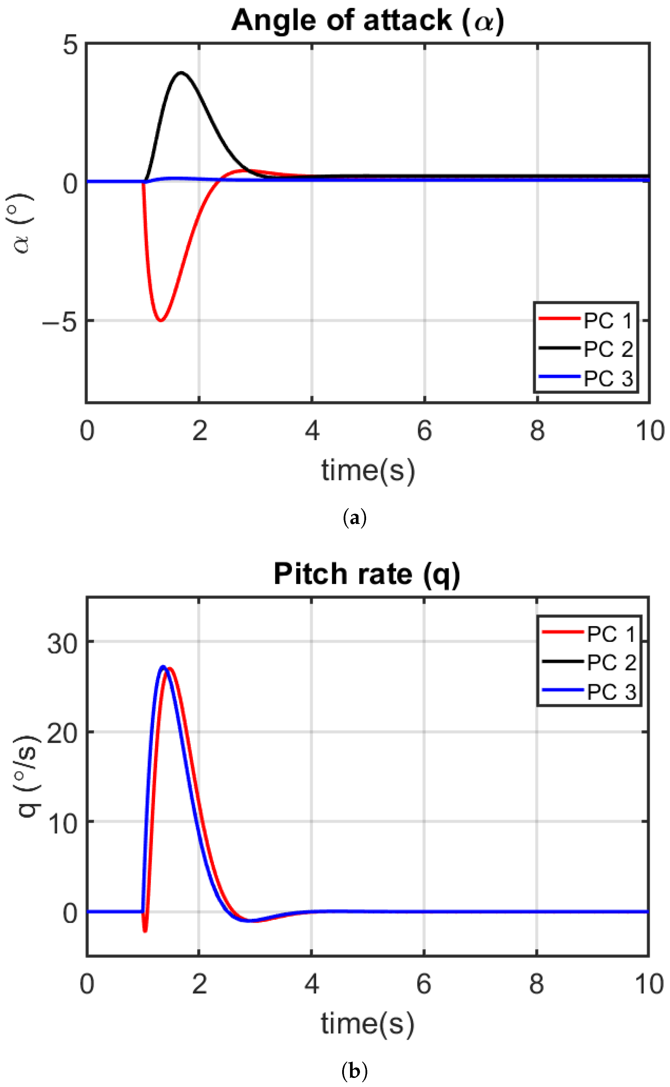
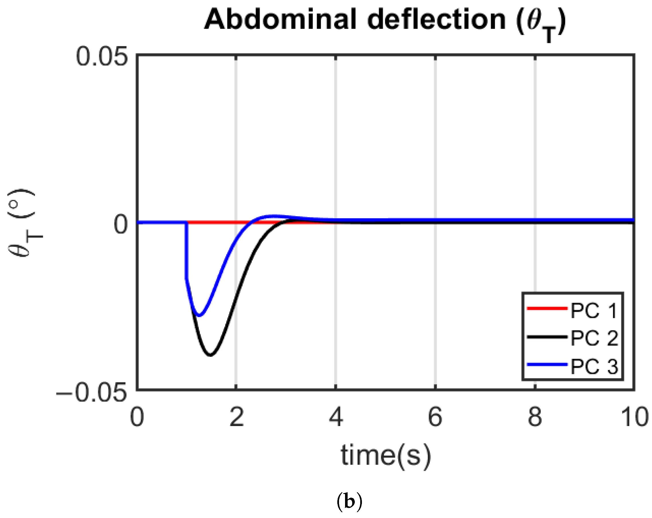
4.5.1. Longitudinal Control Simulation Study

The eigenvalues of the A l o n g matrix of the pre-augmented state–space model shown in Equation (68) indicate that the system is stable since all real parts of the eigenvalues are negative
e i g ( A l o n g ) = 17.73 ± 19.58 i 0.15 ± 0.24 i
For the longitudinal controller, the variable being controlled is the pitch angle; hence, ( y l o n g = e θ ), furthermore, it is assumed that changes in θ do not affect the speed of the aircraft. Therefore, the corresponding axial velocity u components are ignored. In addition, thrust is assumed to be constant, therefore, the effects of changes in thrust are ignored. The z B axis velocity w was replaced with the angle of attack α using the relationship ( α = w u 0 ). The longitudinal augmented states considered are z l o n g = [ α q θ e θ ] , and the longitudinal control inputs: u l o n g = [ δ e θ T ] . The resulting augmented matrices are
A ^ l o n g = 2.66 0.68 0.025 0 67.54 8.74 0.64 0 0 1 0 0 0 0 1 0 ,   B ^ l o n g = 0 0 2.20 1.65 6.43 190.03 0 0 C ^ l o n g = 0 0 0 1 ,   D ^ l o n g = 0 0
The obtained longitudinal linearized model was checked to be controllable and observable using MATLAB functions ctrb ( A ^ l o n g , B ^ l o n g ) and obsv ( A ^ l o n g , C ^ l o n g ) , respectively. The observability and controllability matrices were fully ranked ( r a n k ( O l o n g ) = r a n k ( C l o n g ) = 4 ) . Therefore, the longitudinal model is controllable and observable.
Three pitch control (PC) strategies were investigated based on the selection of weighting matrices R l o n g to reflect the following:
  • PC 1 —Prioritized use of elevator for pitch angle control, interpreted as cheap elevator cost and expensive abdominal pitch cost.
  • PC 2—Prioritized use of abdominal pitch for pitch angle control, interpreted as expensive elevator cost and cheap abdominal pitch cost.
  • PC 3—Relatively evenly prioritized use of elevator and abdominal pitch for pitch angle control, interpreted as cheap elevator cost, cheap abdominal pitch cost.
The same state-weighting matrices Q l o n g = d i a g [ 4 6 4 500 ] , which were selected using Bryson’s rule as a guide [140], were used for all cases considered. Then, the optimal gains were calculated using MATLAB’s lqr (A,B,Q,R) function. A summary of the cases considered for pitch angle control are presented in Table 5. As the control objective was to track a reference pitch angle while keeping all states and control efforts within bounds, the performance characteristics for all cases are compared in terms of settling time, overshoot and steady-state error. The selected gains resulted in the closed-loop step response shown in Figure 4 for the states, while the control efforts are shown in Figure 5. The performance characteristics of the control strategies are summarized in Table 6.

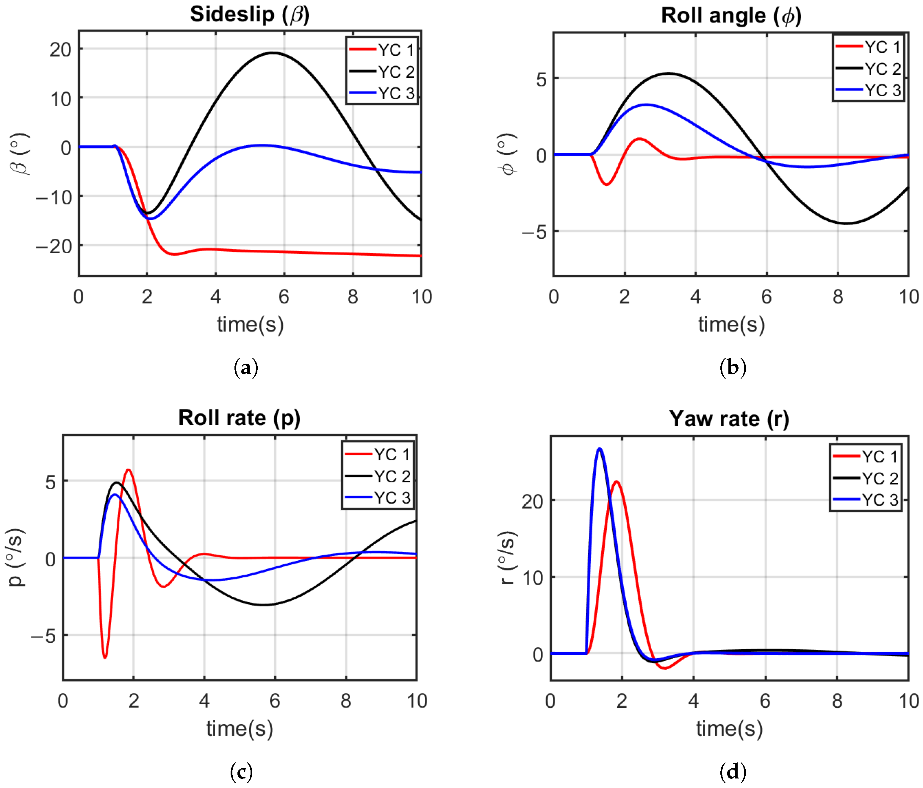
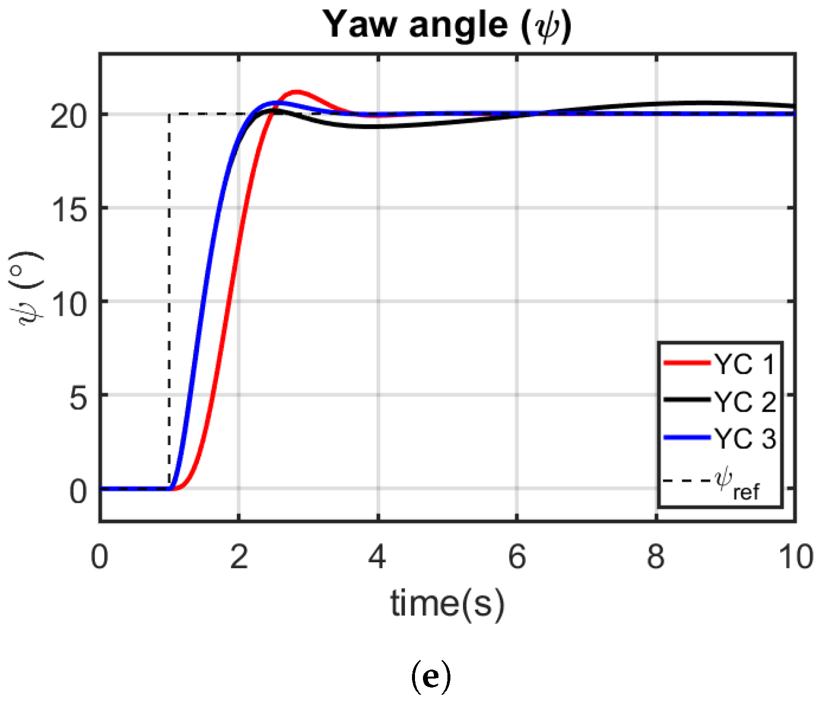
4.5.2. Lateral–Directional Simulation Study

Estimating the eigenvalues of the A l a t matrix of the pre-augmented state–space model in Equation (69) reveals that the system is unstable due to the existence of a positive real part in the characteristic roots.
e i g ( A l a t ) = 1.02 ± 3.67 i 86.05 2.68 0
For the yaw angle controller, the variable being controlled is the yaw angle; hence, ( y l a t = e ψ ). The y B axis velocity v was replaced with the sideslip angle, β , using the relationship β = v u 0 . The lateral augmented states considered were z l a t = [ β p r ϕ ψ e ψ ] , and the control inputs: u l a t = [ δ a ψ T ] . The resulting augmented matrices are
A ^ l a t = 0.025 0.032 0.99 1.22 0 0 14.09 85.94 12.47 0 0 0 0.45 0.014 0.49 23.33 0 0 0 1 0.02 0 0 0 0 0 1 0 0 0 0 0 0 0 1 0 ,   B ^ l a t = 0.032 7.11 18.71 0 0.32 137.27 0 0 0 0 0 0 C ^ l a t = 0 0 0 0 0 1 ,   D ^ l a t = 0 0
Checking the lateral–directional linearized model controllability and observability using MATLAB functions ctrb ( A ^ l a t , B ^ l a t ) and obsv ( A ^ l a t , C ^ l a t ) , respectively resulted in fully ranked matrices ( r a n k ( O l a t ) = r a n k ( C l a t ) = 6 ) . Therefore, the lateral–directional model is controllable and observable.
Again, three yaw control (YC) strategies were investigated based on the selection of weighting matrices R l a t to reflect the following:
  • YC 1—Prioritized use of aileron for yaw angle control, interpreted as cheap aileron cost, expensive abdominal yaw cost.
  • YC 2—Prioritized use of abdominal yaw for yaw angle control, interpreted as expensive aileron cost, cheap abdominal yaw cost.
  • YC 3—Relatively evenly prioritized use of elevator and abdominal pitch for yaw angle control, interpreted as cheap aileron cost, cheap abdominal yaw cost.
The same state-weighing matrix Q l a t = d i a g [ 6 6 6 3 3 500 ] was used for all cases considered. The choice of the state-weighting matrix was also influenced by the need to minimize the sideslip when the aircraft is turning. The estimated optimal gains, as well as other parameters for the yaw controllers, are presented in Table 7. The state trajectory and control effort responses are shown in Figure 6 and Figure 7 respectively. Additionally, a comparison of performance characteristics is presented in Table 8.

5. Discussion

5.1. Model Validation: Single-Body vs. Multibody

As shown in Table 2, the trim results for the DISWA using the single-body model and multibody model are similar at various flight speeds. The only difference is the motor torque τ a y , acting on the abdomen which represents the amount of torque needed to keep the abdominal pitch inclination angle at the specified values and can be treated as a disturbance torque for control purposes.

5.2. Effect of Abdominal Mass on Longitudinal Stability

From the results presented in Table 4, the longitudinal stability of the aircraft decreases with increasing mass of the abdomen. This is associated with the static margin of the aircraft. A statically stable aircraft can be dynamically unstable; however, the reverse is not the case. The aircraft was stable up until 16%; however, as it became statically unstable from 21%, it also became dynamically unstable. Additionally, one can observe two complex conjugate pairs of eigenvalues for the dynamically stable system (6–16%). The highly damped pairs are the short-period modes, and the lightly damped modes represent the phugoid modes. For dynamically unstable systems in general, control systems must be designed that can stabilize the aircraft during flight.

5.3. Pitch Attitude Control

The longitudinal control input plots in Figure 5 show which longitudinal control effectors were prioritized for use in pitch-up control. For PC 1, the elevator was used exclusively, indicated by a downward elevator deflection in Figure 5a, and no abdominal deflection in Figure 5b. PC 2 used abdominal pitch deflection exclusively as seen in Figure 5a, and no elevator deflection in Figure 5b. A downward elevator and upward abdominal pitch deflection shown in Figure 5a,b, respectively, show that the elevator and abdomen were simultaneously used for control in PC 3.
The effects of the control effector choice on longitudinal states over time according to the controller used are shown in Figure 4. The angle of attack α time history in Figure 4a reveals that exclusive use of a positive elevator deflection (PC 1) caused an initial decrease in angle of attack as expected. Similar results have been obtained in [141,142] for tailless aircraft. The deflection of the elevator causes a change in the camber of the airfoil of the wing and consequently changes the lift coefficient. A positive elevator deflection for a reflex airfoil, as in the case of the aircraft wing in this study, decreases the wing lift and pitching moment, therefore resulting in a decrease in angle of attack. However, the exclusive deflection of the abdomen (PC 2) shifts the combined c g forward, and consequently causes a change in lift and drag reference offset, as well as gravitational moments, therefore generating control moments. The resulting effect is the initial increase in angle of attack. In the case of PC 3, these effects are combined and reduced. Regarding the time histories of the pitch rate q (Figure 4b) for the three pitch controllers, an increase in pitch angle resulted in an increase in pitch rate, as expected.
The simulation results presented in Figure 4, Figure 5 and Table 6 showed that the PC 3 controller had better tracking performance for pitch angle than the PC 1 and PC 2 controllers, with a settling time of 2.96 s and the least overshoot of 3.81%. The PC 1 controller was the poorest performer of the three controllers with the highest overshoot of 3.84% and the longest settling time of 3.08 s. All three controllers had zero steady-state error and fall within the set performance requirements. The corresponding control efforts for elevator deflection δ e and abdominal pitch angle are well within the physical bounds with maximum absolute deflections being 0.37 and, 0.04 respectively. The states also fall within the simulation constraints set for α and q, with the maximum absolute values of 5.00 and 27.14 /s, respectively. For parallel comparison, the results indicate that a dragonfly using its abdomen in conjunction with its wings would obtain improved controllability and control performance compared to just using the wings.

5.4. Yaw Attitude Control

Figure 7 shows the lateral–directional control input plots for yaw angle control. YC 1 uses ailerons exclusively and zero abdominal yaw deflection, abdominal yaw deflection exclusively and zero aileron deflection for YC 2, and both aileron and abdominal yaw deflection for YC 3. The transient response for the lateral–directional dynamic response in terms of sideslip angle β , roll angle ϕ and roll rate p are presented in Figure 6a–c. Please note that prior to implementation of a controller, the aircraft was laterally unstable (Equation (73), which is not unusual for tailless aircraft [141,143]. Similar behavior can be observed based on the effect of yaw control effector choice on the transient of these states. The exclusive use of the aileron (YC 1) produces the most stable response in β , ϕ and p, while using the abdominal yaw alone for control (YC 2) caused the aircraft to be more unstable as a result of dynamic effects of the oscillatory movement of the abdomen as seen in Figure 7b. Simultaneously using both ailerons and abdominal yaw (YC 3), on the other hand, reduced the instability experienced with the exclusive use of abdominal yaw in YC 2. The main remark regarding the state evolution of roll angle (Figure 6b) and roll rate (Figure 6c) is the presence of a strong coupling between lateral and directional dynamics, caused by aileron and abdominal yaw deflection.
A yaw controller generates a sideslip to induce a turn and a significant problem associated with turning of a rudderless aircraft is adverse yaw resulting from the differential lift and drag on the left and right wing. The sideslip angle β is a key performance indicator for aircraft turn coordination, i.e., with zero sideslip angle β = 0 . The time history for sideslip angle β in Figure 6a shows that the exclusive use of ailerons (YC 1) and exclusive use of abdominal yaw (YC 2) resulted in negative sideslip. However, simultaneously using ailerons and abdominal yaw achieved better turn coordination over time. Regarding the time histories of the yaw rate r (Figure 6d), for the three yaw controllers, an increase in yaw angle resulted in an increase in yaw rate as expected.
From the simulation results presented in Figure 6, Figure 7 and Table 8, it can be observed that YC 3 has a better response in terms of settling time of 2.29 s compared to that of YC 1 and YC 2 with settling times of 3.33 s and 6.25 s, respectively. In terms of overshoot, YC 2 has the least overshoot 0.89%, compared to YC 1 and YC 3 with overshoots of 5.80% and 2.95%, respectively. YC 2 gives the highest steady-state error of 2%, with the steady-state errors of YC 1 and YC 3 being 0% and 0.04%, respectively. In addition, the corresponding control efforts for aileron deflection δ a and abdominal yaw angle fall within the set limits with maximum absolute deflections being 0.056 and, 0.013 respectively. The states also fall within the simulation constraints set for β , p and r, with maximum absolute values of 22.24 , 6.53 /s and 26.56 /s, respectively. Of all the controllers, only YC 3 meets the controller performance requirements. For insects, the lack of a dedicated yaw-controlling surface similar to the aerodynamic rudder of many aircraft causes inherent instability on the lateral axis; however, “ruddering” movements of the abdomen have been observed [144]. The results attest to the potential use of a yaw-like abdominal airframe-based control mechanism that can be beneficial for the reduction of sideslip during turns (see Figure 6a) as sideslip is a critical control state of the entire aircraft.
The results obtained for yaw control are consistent with the observation in the analysis by Eturk in [36] that used internal moving mass for turn trim and trajectory control. With the internal moving mass, the aircraft was able to achieve trimmed turning flight with no sideslip, which was not possible using conventional aerodynamic control surfaces. Unlike that study, however, reaction torques are apparent, due to the size and mass of the appendage.
The application of an externally articulated mass specifically and solely for lateral control should be designed systematically due to the tendency of the articulated mass in this configuration to reduce the lateral–directional flight quality of a tailless aircraft.

6. Conclusions

A tensor-based multibody flight dynamics simulation model of a dragonfly-inspired straight-flying wing aircraft that considers abdominal articulation was presented in this study. The longitudinal and lateral flight altering effects of the mechanism have been demonstrated dynamically in simulation. An effective pitch and yaw angle tracking controller based on optimal control theory was implemented that was only possible with this new formulation. Allocation of control effort between the moving mass and aerodynamic actuators was achieved using modern control techniques. This control concept offers an alternative to conventional aerodynamic control surfaces for unmanned aerial vehicles. In addition, the results demonstrate the benefit of abdominal articulation of insects or tailless aircraft for longitudinal and lateral attitude control, especially for minimizing sideslip angle during turns.
The aerodynamic effects of the abdomen have been neglected in this study. Future work will extend this model to create a more comprehensive model that incorporates appendage aerodynamics. Although testing was done in the range in which the aircraft had adequate aerodynamic control, it is worth considering the operational range of extremely small aircraft. Furthermore, only one value of actuated mass was considered for control design. Simulation results show the actuated mass ratio to the mass of the aircraft has effects on the control sensitivity of the mechanism. Therefore, control sensitivity may be increased using a heavier mass. Finding an optimal mass for such a mechanism should be considered for future analysis. Additionally, the LQI control design procedure followed in this study can be extended for robustness to include uncertainties and actuator dynamics. Control allocation strategies can also be added to address issues such as actuator input saturation and rate limits, actuator redundancy, and fault tolerance of actuators and effectors.

Author Contributions

Conceptualization, T.O., J.C.; Methodology, T.O.; Execution of study, T.O.; Writing—Original Draft Preparation, T.O. and J.C.; Writing—Review and Editing, T.O., E.A. and J.C. All authors have read and agreed to the published version of the manuscript.

Funding

This research received no external funding.

Data Availability Statement

The simulated data presented in this study are available on request from the corresponding author.

Acknowledgments

T.O. was supported by the Australian Government Research Training Program international (RTPi) scholarship program.

Conflicts of Interest

The authors declare no conflict of interest.

Abbreviations

Acronyms
AoAAngle of Attack
AREAlgebraic Riccati Equation
ARPAerodynamic Reference Point
AVLAthena Vortex Lattice
CAControl Allocation
CoMCenter of Mass
cgCenter of Gravity
DISWADragonfly-Inspired Straight-Wing Aircraft
DoFDegree of Freedom
EoMEquation of Motion
LHSLeft-hand Side
LQILinear Quadratic Integral
LQRLinear Quadratic Regulator
MAVMicro-Aerial Vehicle
MIMOMultiple-input Multiple-output
MMCMoving Mass Control
MPCModel Predictive Control
NPNeutral Point
PCPitch Control
PIDProportional Integral Derivative
RHSRight-Hand Side
SMStatic Margin
SMCSliding Mode Control
SUAVMini Unmanned Aerial Vehicle
wrtWith Respect To
YCYaw Control
Nomenclature
A,OArbitrary rigid bodies A and O (Central body (B), abdomen (T) or aircraft (C) in text) (–), Body-fixed frames associated with rigid bodies A and O (–)
a,oFirst-order tensors (equivalent to a vector) associated with frames A and O (–)
m A , m O Mass of rigid bodies A and O, respectively (kg)
mTotal mass (kg)
[ * ] A Vector or tensor expressed in reference frame A (–)
s a o Displacement vector of point a relative to point b (m)
S a o Skew symmetric matrix of s a o (m)
V A o Velocity of rigid body A relative to point of (m/s)
ω A O Angular velocity of frame A relative to frame O (rad/s)
Ω A O Skew symmetric matrix of ω A O (rad/s)
I a A Inertia tensor of rigid body A about at point a (kg · m 2 )
[ R ] O A Transformation matrix from frame A to O (–)
D A ( * ) Rotational time derivative of a vector or tensor * with respect to frame A (–)
d ( * ) d t Ordinary time derivative of * (–)
eOutput error of additional integral state (–)
gAcceleration due to gravity ( m / s 2 )
iImaginary unit (–)
HAltitude/height (m)
FExternal force vector (N)
MExternal moment vector (N · m)
VAirspeed (m/s)
T n Propulsive thrust (N)
c r e f Reference wing chord (m)
b r e f Reference wing span (m)
S r e f Reference wing area ( m 2 )
C ( x , y , z ) Dimensionless aerodynamic coefficients for axial, side and normal force, respectively (–)
C ( l , m , n ) Dimensionless aerodynamic coefficients for roll, pitch and yaw moment, respectively (–)
u , v , w Velocity vector components (m/s)
p , q , r Angular velocity vector components (rad/s)
X , Y , Z Position vector components (m)
α , β Angle of Attack and sideslip angle (rad)
δ r Elevator deflection angle (rad)
δ e Aileron deflection angle (rad)
η Elevon deflection angle (rad)
κ Damping constant (N · m · s)
ρ Air density ( kg / m 3 )
τ l Load torque due to gravity (N · m)
τ a Actuator torque (N · m)
ϕ , θ , ψ Roll, pitch and yaw Euler angles (rad)
x , u , z state, input, output vector (–)
r , y Reference input signal, output signal (–)
A , B , C , D System state, control, output and feedforward matrices (–)
K Optimal gain matrix (–)
Q State-weighting matrix (–)
R Control weighting matrix (–)
J Cost function (–)
P Algebraic Riccati Equation solution (–)
Subscripts
0Initial/nominal value
iAdditional integral states
k k t h rigid body
B, TCentral rigid body, abdomen rigid body
I, B, TInertial, central body and abdominal reference frames systems
l, rleft, right
latLateral–directional motion
longLongitudinal motion
Superscripts
˙ First-order time derivative
¨ Second-order time derivative
^ Augmented matrix
Transpose of parameter
1 Inverse of parameter

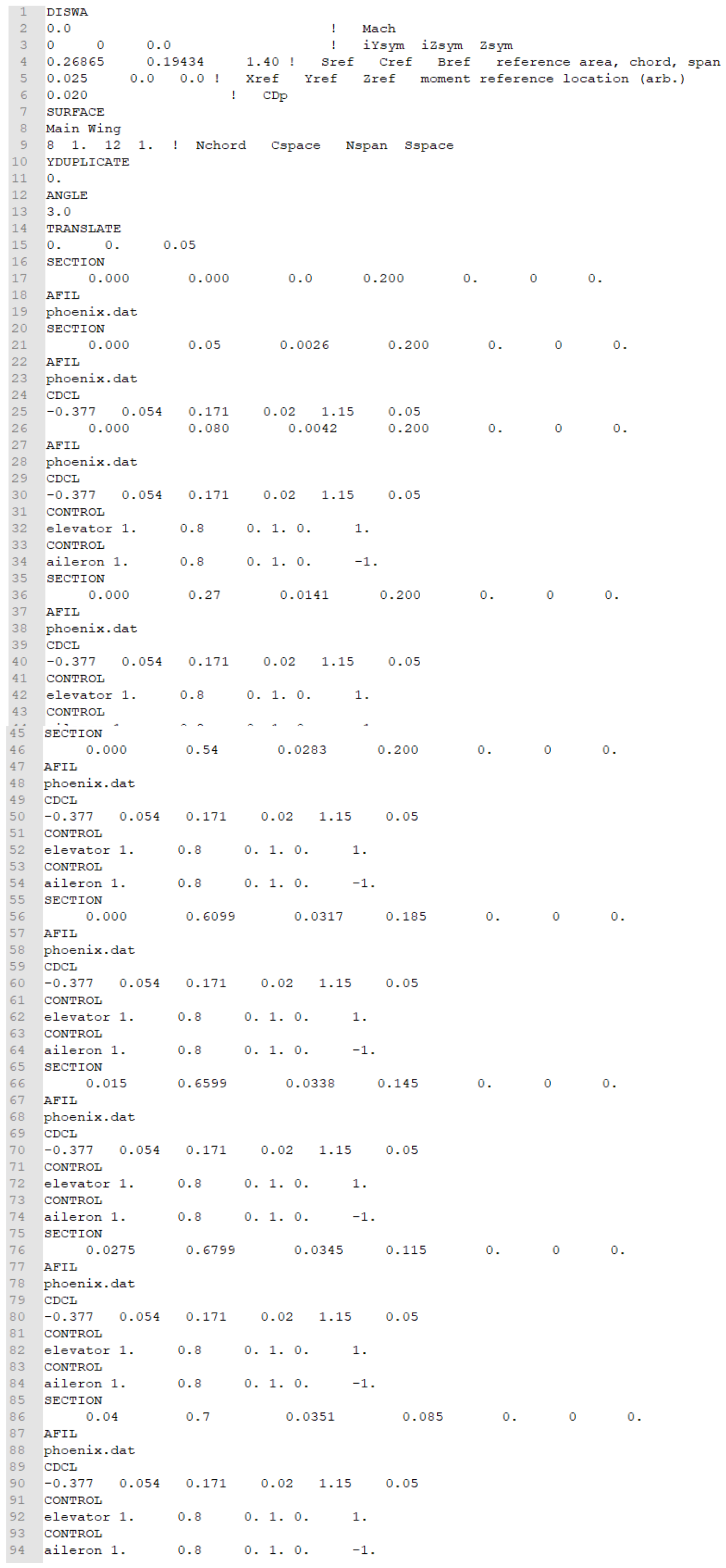
Appendix A. Athena Vortex Lattice File for Aerodynamic Data

Below (Figure A1) is the AVL input geometry file used to generate the aerodynamic data of the DISWA used in this study. The aerodynamic coefficients and stability derivatives are functions of the aerodynamic angles. To generate the data as a function of the angle of attack for instance, AVL is capable of sweeping through a range of AoA. More information on how to use the AVL tool can be found in [137].
Figure A1. DISWA AVL input geometry file.
Applsci 12 01162 g0a1

References

  1. Ramesh, P.; Jeyan, M.L. Mini Unmanned Aerial Systems (UAV)—A Review of the Parameters for Classification of a Mini UAV. Int. J. Aviat. Aeronaut. Aerosp. 2020, 7, 5. [Google Scholar]
  2. Alexander, R.M. Principles of Animal Locomotion; Princeton University Press: Princeton, NJ, USA, 2013. [Google Scholar]
  3. Ellington, C.P. The aerodynamics of hovering insect flight. IV. Aerodynamic mechanisms. Philos. Trans. R. Soc. Lond. Biol. Sci. 1984, 305, 79–113. [Google Scholar]
  4. Ellington, C.P. The aerodynamics of hovering insect flight. VI. Lift and power requirements. Philos. Trans. R. Soc. Lond. Biol. Sci. 1984, 305, 145–181. [Google Scholar]
  5. Pennycuick, C.J. A wind-tunnel study of gliding flight in the pigeon Columba livia. J. Exp. Biol. 1968, 49, 509–526. [Google Scholar] [CrossRef]
  6. Pennycuick, C.J. Control of gliding angle in Rüppell’s griffon vulture Gyps rueppelli. J. Exp. Biol. 1971, 55, 39–46. [Google Scholar] [CrossRef]
  7. Cook, M.; Spottiswoode, M. Modelling the flight dynamics of the hang glider. Aeronaut. J. 2005, 109, I–XX. [Google Scholar] [CrossRef] [Green Version]
  8. Libby, T.; Moore, T.Y.; Chang-Siu, E.; Li, D.; Cohen, D.J.; Jusufi, A.; Full, R.J. Tail-assisted pitch control in lizards, robots and dinosaurs. Nature 2012, 481, 181. [Google Scholar] [CrossRef]
  9. Chahl, J.; Chitsaz, N.; McIvor, B.; Ogunwa, T.; Kok, J.M.; McIntyre, T.; Abdullah, E. Biomimetic Drones Inspired by Dragonflies Will Require a Systems Based Approach and Insights from Biology. Drones 2021, 5, 24. [Google Scholar] [CrossRef]
  10. Götz, K.G.; Hengstenberg, B.; Biesinger, R. Optomotor control of wing beat and body posture in Drosophila. Biol. Cybern. 1979, 35, 101–112. [Google Scholar] [CrossRef]
  11. Zanker, J. On the mechanism of speed and altitude control in Drosophila melanogaster. Physiol. Entomol. 1988, 13, 351–361. [Google Scholar] [CrossRef]
  12. Berthé, R.; Lehmann, F.O. Body appendages fine-tune posture and moments in freely manoeuvring fruit flies. J. Exp. Biol. 2015, 218, 3295–3307. [Google Scholar] [CrossRef] [PubMed] [Green Version]
  13. Zanker, J.M.; Egelhaaf, M.; Warzecha, A.K. On the coordination of motor output during visual flight control of flies. J. Comp. Physiol. 1991, 169, 127–134. [Google Scholar] [CrossRef] [Green Version]
  14. Combes, S.A.; Dudley, R. Turbulence-driven instabilities limit insect flight performance. Proc. Natl. Acad. Sci. USA 2009, 106, 9105–9108. [Google Scholar] [CrossRef] [PubMed] [Green Version]
  15. Cheng, B.; Deng, X.; Hedrick, T.L. The mechanics and control of pitching manoeuvres in a freely flying hawkmoth (Manduca sexta). J. Exp. Biol. 2011, 214, 4092–4106. [Google Scholar] [CrossRef] [Green Version]
  16. Hedrick, T.L.; Daniel, T.L. Flight control in the hawkmoth Manduca sexta: The inverse problem of hovering. J. Exp. Biol. 2006, 209, 3114–3130. [Google Scholar] [CrossRef] [Green Version]
  17. Luu, T.; Cheung, A.; Ball, D.; Srinivasan, M.V. Honeybee flight: A novel ‘streamlining’ response. J. Exp. Biol. 2011, 214, 2215–2225. [Google Scholar] [CrossRef] [Green Version]
  18. Sridhar, M.; Kang, C.K.; Lee, T. Geometric Formulation for the Dynamics of Monarch Butterfly with the Effects of Abdomen Undulation. In Proceedings of the AIAA Scitech 2020 Forum, Orlando, FL, USA, 6–10 January 2020; p. 1962. [Google Scholar]
  19. Rüppell, G.; Hilfert-Rüppell, D.; Schneider, B.; Dedenbach, H. On the firing line–interactions between hunting frogs and Odonata. Int. J. Odonatol. 2020, 23, 1–19. [Google Scholar] [CrossRef]
  20. Bode-Oke, A.T.; Zeyghami, S.; Dong, H. Flying in reverse: Kinematics and aerodynamics of a dragonfly in backward free flight. J. R. Soc. Interface 2018, 15, 20180102. [Google Scholar] [CrossRef]
  21. Zanker, J.M. How does lateral abdomen deflection contribute to flight control of Drosophila melanogaster? J. Comp. Physiol. 1988, 162, 581–588. [Google Scholar] [CrossRef]
  22. Dyhr, J.P.; Morgansen, K.A.; Daniel, T.L.; Cowan, N.J. Flexible strategies for flight control: An active role for the abdomen. J. Exp. Biol. 2013, 216, 1523–1536. [Google Scholar] [CrossRef] [Green Version]
  23. Hinterwirth, A.J.; Daniel, T.L. Antennae in the hawkmoth Manduca sexta (Lepidoptera, Sphingidae) mediate abdominal flexion in response to mechanical stimuli. J. Comp. Physiol. 2010, 196, 947–956. [Google Scholar] [CrossRef] [PubMed]
  24. Frye, M.A. Effects of stretch receptor ablation on the optomotor control of lift in the hawkmoth Manduca sexta. J. Exp. Biol. 2001, 204, 3683–3691. [Google Scholar] [CrossRef] [PubMed]
  25. Dyhr, J.P.; Cowan, N.J.; Colmenares, D.J.; Morgansen, K.A.; Daniel, T.L. Autostabilizing airframe articulation: Animal inspired air vehicle control. In Proceedings of the 2012 IEEE 51st IEEE Conference on Decision and Control (CDC), Maui, HI, USA, 10–13 December 2012; pp. 3715–3720. [Google Scholar]
  26. Arbas, E.A. Control of hindlimb posture by wind-sensitive hairs and antennae during locust flight. J. Comp. Physiol. 1986, 159, 849–857. [Google Scholar] [CrossRef] [PubMed]
  27. Camhi, J.M. Sensory control of abdomen posture in flying locusts. J. Exp. Biol. 1970, 52, 533–537. [Google Scholar] [CrossRef]
  28. Camhi, J.M. Yaw-correcting postural changes in locusts. J. Exp. Biol. 1970, 52, 519–531. [Google Scholar] [CrossRef]
  29. Tejaswi, K.; Kang, C.k.; Lee, T. Dynamics and control of a flapping wing uav with abdomen undulation inspired by monarch butterfly. In Proceedings of the 2021 American Control Conference (ACC), New Orleans, LA, USA, 25–28 May 2021; pp. 66–71. [Google Scholar]
  30. Tejaswi, K.; Sridhar, M.K.; Kang, C.k.; Lee, T. Effects of abdomen undulation in energy consumption and stability for monarch butterfly. Bioinspir. Biomimetic 2021, 16, 046003. [Google Scholar]
  31. Jang, J.; Tomlin, C. Longitudinal stability augmentation system design for the DragonFly UAV using a single GPS receiver. In Proceedings of the AIAA Guidance, Navigation, and Control Conference and Exhibit, Austin, TX, USA, 11–14 August 2003; p. 5592. [Google Scholar]
  32. Couceiro, M.S.; Ferreira, N.; Tenreiro Machado, J.A. Modeling and control of a dragonfly-like robot. J. Control. Sci. Eng. 2010, 2010, 643045. [Google Scholar] [CrossRef] [Green Version]
  33. Nguyen, Q.V.; Chan, W.L.; Debiasi, M. Design, fabrication, and performance test of a hovering-based flapping-wing micro air vehicle capable of sustained and controlled flight. In Proceedings of the IMAV 2014: International Micro Air Vehicle Conference and Competition 2014, Delft, The Netherlands, 12–15 August 2014; Delft University of Technology: Delft, The Netherlands, 2014. [Google Scholar]
  34. Siqueira, J.C.D.C. Modeling of Wind Phenomena and Analysis of Their Effects on UAV Trajectory Tracking Performance. Ph.D. Thesis, West Virginia University, Morgantown, WV, USA, 2017. [Google Scholar]
  35. Gebert, G.; Gallmeier, P.; Evers, J. Equations of motion for flapping flight. In Proceedings of the AIAA Atmospheric Flight Mechanics Conference and Exhibit, Monterey, CA, USA, 6 August 2002; p. 4872. [Google Scholar]
  36. Erturk, S.A. Performance Analysis, Dynamic Simulation and Control of Mass-Actuated Airplane. Ph.D. Thesis, University of Texas at Arlington, Arlington, TX, USA, 2016. [Google Scholar]
  37. Haixu, L.; Xiangju, Q.; Weijun, W. Multi-body motion modeling and simulation for tilt rotor aircraft. Chin. J. Aeronaut. 2010, 23, 415–422. [Google Scholar] [CrossRef] [Green Version]
  38. Sakhaei, A. Dynamic Modelling and Predictive Control for Insect-like Flapping Wing Aerial Micro Robots. Ph.D. Thesis, Ryerson University, Toronto, ON, Canada, 2010. [Google Scholar]
  39. Grauer, J.; Ulrich, E.; Hubbard, J.; Pines, D.; Humbert, J. System identification of an ornithopter aerodynamics model. In Proceedings of the AIAA Atmospheric Flight Mechanics Conference, Toronto, ON, Canada, 2–5 August 2010; p. 7632. [Google Scholar]
  40. Grauer, J.; Ulrich, E.; Hubbard Jr, J.; Pines, D.; Humbert, J.S. Testing and system identification of an ornithopter in longitudinal flight. J. Aircr. 2011, 48, 660–667. [Google Scholar]
  41. Orlowski, C.; Girard, A.; Shyy, W. Open loop pitch control of a flapping wing micro-air vehicle using a tail and control mass. In Proceedings of the 2010 American Control Conference, Baltimore, MA, USA, 30 June–2 July 2010; pp. 536–541. [Google Scholar]
  42. Caetano, J.; Weehuizen, M.; De Visser, C.; De Croon, G.; De Wagter, C.; Remes, B.; Mulder, M. Rigid vs. flapping: The effects of kinematic formulations in force determination of a free flying Flapping Wing Micro Air Vehicle. In Proceedings of the 2014 International Conference on Unmanned Aircraft Systems (ICUAS), Orlando, FL, USA, 27–30 May 2014; pp. 949–959. [Google Scholar]
  43. Bolender, M. Rigid multi-body equations-of-motion for flapping wing mavs using kane’s equations. In Proceedings of the AIAA Guidance, Navigation, and Control Conference, Chicago, IL, USA, 11 August 2009; p. 6158. [Google Scholar]
  44. Su, J.; Su, C.; Xu, S.; Yang, X. A multibody model of tilt-rotor aircraft based on Kane’s method. Int. J. Aerosp. Eng. 2019, 2019, 9396352. [Google Scholar] [CrossRef] [Green Version]
  45. Lasek, M.; Sibilski, K. Modelling and simulation of flapping wing control for a micromechanical flying insect (entomopter). In Proceedings of the AIAA Modeling and Simulation Technologies Conference and Exhibit, Monterey, CA, USA, 5–8 August 2002; p. 4973. [Google Scholar]
  46. Sibilski, K.; Loroch, L.; Buler, W.; Zyluk, A. Modeling and simulation of the nonlinear dynamic behavior of a flapping wings micro-aerial-vehicle. In Proceedings of the 42nd AIAA Aerospace Sciences Meeting and Exhibit, Reno, NV, USA, 5–8 January 2004; p. 541. [Google Scholar]
  47. Grauer, J.A.; Hubbard, J.E., Jr. Multibody model of an ornithopter. J. Guid. Control Dyn. 2009, 32, 1675–1679. [Google Scholar] [CrossRef]
  48. Sun, M.; Wang, J.; Xiong, Y. Dynamic flight stability of hovering insects. Acta Mech. Sin. 2007, 23, 231–246. [Google Scholar] [CrossRef]
  49. Loh, K.; Cook, M.; Thomasson, P. An investigation into the longitudinal dynamics and control of a flapping wing micro air vehicle at hovering flight. Aeronaut. J. 2003, 107, 743–753. [Google Scholar]
  50. Orlowski, C.T. Flapping Wing Micro Air Vehicles: An Analysis of the Importance of the Mass of the Wings to Flight Dynamics, Stability, and Control. Ph.D. Thesis, University of Michigan, Ann Arbor, MI, USA, 2011. [Google Scholar]
  51. Du, C.; Xu, J.; Zheng, Y. Modeling and control of a dragonfly-like micro aerial vehicle. Adv. Robot Autom. S 2015, 2, 2. [Google Scholar]
  52. Grubin, C. Dynamics of a vehicle containing moving parts. J. Appl. Mech. 1962, 29, 486–488. [Google Scholar] [CrossRef]
  53. Janssens, F.L.; van der Ha, J.C. Stability of spinning satellite under axial thrust, internal mass motion, and damping. J. Guid. Control Dyn. 2015, 38, 761–771. [Google Scholar] [CrossRef]
  54. Mingori, D.; Yam, Y. Nutational stability of a spinning spacecraft with internal mass motion and axial thrust. In Proceedings of the Astrodynamics Conference, Vail, CO, USA, 12 August 1986; p. 2271. [Google Scholar]
  55. Mingori, D.; Halsmer, D.; Yam, Y. Stability of spinning rockets with internal mass motion. NASA Sti/Recon Tech. Rep. 1993, 95, 199–209. [Google Scholar]
  56. Yam, Y.; Mingori, D.; Halsmer, D. Stability of a spinning axisymmetric rocket with dissipative internal mass motion. J. Guid. Control Dyn. 1997, 20, 306–312. [Google Scholar] [CrossRef]
  57. Salimov, G. Motion of a spacecraft containing a moving element in a gravitational field. Mekhanika Tverd. Tela 1974, 9, 35–41. [Google Scholar]
  58. Leshchenko, D. Motion of a rigid body with movable point mass. Mekhanika Tverd. Tela 1976, 11, 37–40. [Google Scholar]
  59. Salimov, G. Stability of rotating space station containing a moving element. Mekhanika Tverd. Tela 1975, 10, 52–56. [Google Scholar]
  60. Chernousko, F.L.; Akulenko, L.D.; Leshchenko, D.D. Evolution of Motions of a Rigid Body about Its Center of Mass; Springer: Berlin/Heidelberg, Germany, 2017. [Google Scholar]
  61. Han, J.; Hong, G. Modeling of aircraft with time-varying inertia properties. In Proceedings of the AIAA Modeling and Simulation Technologies Conference, Dallas, TX, USA, 23 June 2015; p. 1133. [Google Scholar]
  62. Roberson, R.E. Torques on a satellite vehicle from internal moving parts. J. Appl. Mech. 1958, 25, 196–200. [Google Scholar] [CrossRef]
  63. Chanute, O. Progress in Flying Machines. Republication of the Work First Published in 1884; Dover Publications: New York, NY, USA, 1997. [Google Scholar]
  64. Wolko, H.S.; Anderson, J. The Wright Flyer: An Engineering Perspective; Smithsonia: Birmingham, UK, 1983. [Google Scholar]
  65. Qin, L.; Yang, M. Moving mass attitude law based on neural networks. In Proceedings of the 2007 International Conference on Machine Learning and Cybernetics, Hong Kong, China, 19–22 August 2007; Volume 5, pp. 2791–2795. [Google Scholar]
  66. Gao, F.J.; Zhao, L.Y. Adaptive sliding mode control with backstepping approach for a moving mass hypersonic spinning missile. In Proceedings of the International Conference on Applied Science and Engineering Innovation (ASEI 2015), Jinan, China, 30–31 August 2015; pp. 834–837. [Google Scholar]
  67. Yi, Y.; Zhou, F. Variable centroid control scheme over hypersonic tactical missile. Sci. China Ser. 2003, 46, 561–569. [Google Scholar]
  68. Rogers, J.; Costello, M. A variable stability projectile using an internal moving mass. Proc. Inst. Mech. Eng. Part J. Aerosp. Eng. 2009, 223, 927–938. [Google Scholar] [CrossRef]
  69. Rogers, J. Applications of Internal Translating Mass Technologies to Smart Weapons Systems; Georgia Institute of Technology: Atlanta, GA, USA, 2009. [Google Scholar]
  70. Rogers, J.; Costello, M. Control authority of a projectile equipped with a controllable internal translating mass. J. Guid. Control Dyn. 2008, 31, 1323–1333. [Google Scholar] [CrossRef]
  71. Wang, S.; Yang, M.; Wang, Z. Moving-mass trim control system design for spinning vehicles. In Proceedings of the 2006 6th World Congress on Intelligent Control and Automation, Dalian, China, 21–23 June 2006; Volume 1, pp. 1034–1038. [Google Scholar]
  72. Chen, L.; Zhou, G.; Yan, X.; Duan, D. Composite control of stratospheric airships with moving masses. J. Aircr. 2012, 49, 794–801. [Google Scholar] [CrossRef]
  73. Vengate, S.R.; Erturk, S.A.; Dogan, A. Development and flight test of moving-mass actuated unmanned aerial vehicle. In Proceedings of the AIAA Atmospheric Flight Mechanics Conference, Washington, DC, USA, 13 June 2016; p. 3713. [Google Scholar]
  74. Haus, T.; Orsag, M.; Bogdan, S. Mathematical modelling and control of an unmanned aerial vehicle with moving mass control concept. J. Intell. Robot. Syst. 2017, 88, 219. [Google Scholar] [CrossRef]
  75. Haus, T.; Orsag, M.; Bogdan, S. Design considerations for a large quadrotor with moving mass control. In Proceedings of the 2016 International Conference on Unmanned Aircraft Systems, Arlington, VA, USA, 7–10 June 2016; pp. 1327–1334. [Google Scholar]
  76. Bouabdallah, S.; Siegwart, R.; Caprari, G. Design and control of an indoor coaxial helicopter. In Proceedings of the 2006 IEEE/RSJ International Conference on Intelligent Robots and Systems, Beijing, China, 9–13 October 2006; pp. 2930–2935. [Google Scholar]
  77. Bermes, C.; Leutenegger, S.; Bouabdallah, S.; Schafroth, D.; Siegwart, R. New design of the steering mechanism for a mini coaxial helicopter. In Proceedings of the 2008 IEEE/RSJ International Conference on Intelligent Robots and Systems, Nice, France, 7 September 2008; pp. 1236–1241. [Google Scholar]
  78. Canuto, E.; Novara, C.; Carlucci, D.; Montenegro, C.P.; Massotti, L. Spacecraft Dynamics and Control: The Embedded Model Control Approach; Butterworth-Heinemann: Oxford, UK, 2018. [Google Scholar]
  79. Virgili-Llop, J.; Polat, H.C.; Romano, M. Attitude stabilization of spacecraft in very low earth orbit by center-of-mass shifting. Front. Robot. 2019, 6, 7. [Google Scholar] [CrossRef] [PubMed] [Green Version]
  80. Childs, D. An Investigation of a Movable Mass-Attitude Stabilization System for Artificial-G Space. J. Spacecr. 1972, 8, 8. [Google Scholar]
  81. Childs, D.W.; Hardison, T.L. A Movable-Mass Attitude Stabilization System For Cable-Connected Artificial-G Space Stations. J. Spacecr. Rocket. 1974, 11, 165–172. [Google Scholar] [CrossRef]
  82. Childs, D.W. A movable-mass attitude-stabilization system for artificial-g space stations. J. Spacecr. Rocket. 1971, 8, 829–834. [Google Scholar] [CrossRef]
  83. Zheng, Q.; Zhou, Z. Stability of Moving Mass Control Spinning Missiles with Angular Rate Loops. Math. Probl. Eng. 2019, 2019. [Google Scholar] [CrossRef] [Green Version]
  84. Li, J.; Gao, C.; Li, C.; Jing, W. A survey on moving mass control technology. Aerosp. Sci. Technol. 2018, 82, 594–606. [Google Scholar] [CrossRef]
  85. Gao, C.; Jing, W.; Wei, P. Research on application of single moving mass in the reentry warhead maneuver. Aerosp. Sci. Technol. 2013, 30, 108–118. [Google Scholar] [CrossRef]
  86. Su, X.L.; Yu, J.Q.; Wang, Y.F.; Wang, L.l. Moving mass actuated reentry vehicle control based on trajectory linearization. Int. J. Aeronaut. Space Sci. 2013, 14, 247–255. [Google Scholar] [CrossRef] [Green Version]
  87. Candel, S. Concorde and the future of supersonic transport. J. Propuls. Power 2004, 20, 59–68. [Google Scholar] [CrossRef]
  88. Turner, H. Fuel management for Concorde: A brief account of the fuel system and the fuel pumps developed for the aircraft. Aircr. Eng. Aerosp. Technol. 1971, 43, 36–39. [Google Scholar] [CrossRef]
  89. Collard, D. Concorde airframe design and development. SAE Trans. 1991, 100, 2620–2641. [Google Scholar]
  90. Seisan, F.Z. Modeling and Control of a Co-Axial Helicopter; University of Toronto (Canada): Toront, ON, Canada, 2012. [Google Scholar]
  91. Graver, J.G. Underwater Gliders: Dynamics, Control and Design. Ph.D. Thesis, Princeton University, Princeton, NJ, USA, 2005. [Google Scholar]
  92. Zhang, X.Y.; Zhao, Y.X.; Xu, D.X.; He, K.P. Sliding mode control for mass moment aerospace vehicles using dynamic inversion approach. Math. Probl. Eng. 2013, 2013, 284869. [Google Scholar] [CrossRef]
  93. Kunciw, B.G. Optimal Detumbling of a Large Manned Spacecraft Using an Internal Moving Mass; The Pennsylvania State University: State College, PA, USA, 1973. [Google Scholar]
  94. Ross, I.M. Mechanism for precision orbit control with applications to formation keeping. J. Guid. Control Dyn. 2002, 25, 818–820. [Google Scholar] [CrossRef]
  95. Beyer, E.W. Design, Testing, and Performance of a Hybrid Micro Vehicle—The Hopping Rotochute; Georgia Institute of Technology: Atlanta, GA, USA, 2009. [Google Scholar]
  96. Nelson, R.C. Flight Stability and Automatic Control; WCB/McGraw Hill: New York, NY, USA, 1998; Volume 2. [Google Scholar]
  97. Chrif, L.; Kadda, Z.M. Aircraft control system using LQG and LQR controller with optimal estimation-Kalman filter design. Procedia Eng. 2014, 80, 245–257. [Google Scholar] [CrossRef] [Green Version]
  98. Shaji, J.; Aswin, R. Pitch control of flight system using dynamic inversion and pid controller. Int. J. Eng. Res. Technol. 2015, 4, 1–5. [Google Scholar] [CrossRef]
  99. Lungu, R.; Lungu, M.; Grigorie, L.T. Automatic control of aircraft in longitudinal plane during landing. IEEE Trans. Aerosp. Electron. Syst. 2013, 49, 1338–1350. [Google Scholar] [CrossRef]
  100. Islam, M.T.; Alam, M.S.; Laskar, M.A.R.; Garg, A. Modeling and simulation of longitudinal autopilot for general aviation aircraft. In Proceedings of the 2016 5th International Conference on Informatics, Electronics and Vision (ICIEV), Piscataway, NJ, USA, 3–14 May 2016; pp. 490–495. [Google Scholar]
  101. Wahid, N.; Hassan, N. Self-tuning fuzzy PID controller design for aircraft pitch control. In Proceedings of the 2012 Third International Conference on Intelligent Systems Modelling and Simulation, Kota Kinabalu, Malaysia, 8–10 February 2012; pp. 19–24. [Google Scholar]
  102. Vishal; Ohri, J. GA tuned LQR and PID controller for aircraft pitch control. In Proceedings of the 2014 IEEE 6th India International Conference on Power Electronics (IICPE), Kurukshetra, India, 8–10 December 2014; pp. 1–6. [Google Scholar]
  103. Ibrahim, I.; Al Akkad, M. Exploiting an intelligent fuzzy-PID system in nonlinear aircraft pitch control. In Proceedings of the 2016 International Siberian Conference on Control and Communications (SIBCON), Russia, Moscow, 12–14 May 2016; pp. 1–7. [Google Scholar]
  104. Babar, M.; Ali, S.; Shah, M.; Samar, R.; Bhatti, A.; Afzal, W. Robust control of UAVs using H∞ control paradigm. In Proceedings of the 2013 IEEE 9th International Conference on Emerging Technologies (ICET), Islamabad, Pakistan, 9–10 December 2013; pp. 1–5. [Google Scholar]
  105. López, J.; Dormido, R.; Dormido, S.; Gómez, J. A robust controller for an UAV flight control system. Sci. World J. 2015, 2015, 403236. [Google Scholar] [CrossRef] [Green Version]
  106. Doyle, J.; Glover, K.; Kh&gaoeSar, P.; Francis, B. StateSpace Solutions to Standard Hi aid Control Problems. IEEE Trans. Autom. Control 1989, 34, 831–847. [Google Scholar] [CrossRef]
  107. Polas, M.; Fekih, A. A multi-gain sliding mode based controller for the pitch angle control of a civil aircraft. In Proceedings of the 2010 42nd Southeastern Symposium on System Theory (SSST), Tyler, TX, USA, 7–9 March 2010; pp. 96–101. [Google Scholar]
  108. Promtun, E.; Seshagiri, S. Sliding mode control of pitch-rate of an f-16 aircraft. IFAC Proc. Vol. 2008, 41, 1099–1104. [Google Scholar] [CrossRef] [Green Version]
  109. MacKunis, W.; Patre, P.M.; Kaiser, M.K.; Dixon, W.E. Asymptotic tracking for aircraft via robust and adaptive dynamic inversion methods. IEEE Trans. Control. Syst. Technol. 2010, 18, 1448–1456. [Google Scholar] [CrossRef] [Green Version]
  110. Wahid, N.; Rahmat, M.F. Pitch control system using LQR and Fuzzy Logic Controller. In Proceedings of the 2010 IEEE Symposium on Industrial Electronics and Applications (ISIEA), Penang, Malaysia, 3–5 October 2010; pp. 389–394. [Google Scholar]
  111. Călugăru, G.; Dănişor, E.A. Improved aircraft attitude control using generalized predictive control method. In Proceedings of the 2016 17th International Carpathian Control Conference (ICCC), High Tatras, Slovakia, 29 May–1 June 2016; pp. 101–106. [Google Scholar]
  112. Härkegård, O. Backstepping and Control Allocation with Applications to Flight Control. Ph.D. Thesis, Linköpings Universitet, Linköping, Sweden, 2003. [Google Scholar]
  113. Härkegård, O. Quadratic Programming Control Allocation Toolbox(Qcat). Mar. Available online: http://research.harkegard.se/qcat (accessed on 12 June 2020).
  114. Luo, Y.; Serrani, A.; Yurkovich, S.; Oppenheimer, M.W.; Doman, D.B. Model-predictive dynamic control allocation scheme for reentry vehicles. J. Guid. Control Dyn. 2007, 30, 100–113. [Google Scholar] [CrossRef]
  115. Bolender, M.A.; Doman, D.B. Nonlinear control allocation using piecewise linear functions: A linear programming approach. J. Guid. Control Dyn. 2005, 28, 558–562. [Google Scholar] [CrossRef] [Green Version]
  116. Durham, W.; Bordignon, K.A.; Beck, R. Aircraft Control Allocation; John Wiley & Sons: Hoboken, NJ, USA, 2017. [Google Scholar]
  117. Buffington, J.M.; Enns, D.F. Lyapunov stability analysis of daisy chain control allocation. J. Guid. Control Dyn. 1996, 19, 1226–1230. [Google Scholar] [CrossRef]
  118. Rupp, A. Control Allocation for Over-Actuated Road Vehicles; University of Graz: Graz, Austria, 2013; pp. 13–26. [Google Scholar]
  119. Oppenheimer, M.W.; Doman, D.B.; Bolender, M.A. Control allocation for over-actuated systems. In Proceedings of the 2006 14th Mediterranean Conference on Control and Automation, Ancona, Italy, 28–26 June 2006; pp. 1–6. [Google Scholar]
  120. Nel, A.; Prokop, J.; Pecharová, M.; Engel, M.S.; Garrouste, R. Palaeozoic giant dragonflies were hawker predators. Sci. Rep. 2018, 8, 12141. [Google Scholar] [CrossRef] [PubMed]
  121. May, M.L. A critical overview of progress in studies of migration of dragonflies (Odonata: Anisoptera), with emphasis on North America. J. Insect Conserv. 2013, 17, 1–15. [Google Scholar] [CrossRef] [Green Version]
  122. Azuma, A.; Watanabe, T. Flight performance of a dragonfly. J. Exp. Biol. 1988, 137, 221–252. [Google Scholar] [CrossRef]
  123. Wakeling, J.; Ellington, C.P. Dragonfly flight. I. Gliding flight and steady-state aerodynamic forces. J. Exp. Biol. 1997, 200, 543–556. [Google Scholar] [CrossRef] [PubMed]
  124. Newman, B. Model test on a wing section of a dragonfly. In Scale Effects in Animal Locomotion; Academic Press: London, UK, 1977; pp. 445–477. [Google Scholar]
  125. Zipfel, P.H. Modeling and Simulation of Aerospace Vehicle Dynamics; American Institute of Aeronautics and Astronautics: Reston, VA, USA, 2007. [Google Scholar]
  126. Wrede, R.C. Introduction to Vector and Tensor Analysis; Wiley: New York, NY, USA, 1963. [Google Scholar]
  127. Beard, R.W.; McLain, T.W. Small Unmanned Aircraft: Theory and Practice; Princeton University Press: Prentice, NJ, USA, 2012. [Google Scholar]
  128. Anderson, B.D.; Moore, J.B. Optimal Control Linear Quadratic Methods; Prentice Hall International: Prentice, NJ, USA, 1989; Volume 7632. [Google Scholar]
  129. Dorato, P.; Cerone, V.; Abdallah, C. Linear Quadratic Control: An Introduction; Krieger Pub Co.: Malabar, FL, USA, 2000. [Google Scholar]
  130. MATLAB. 9.7.0.1190202 (R2019b); The MathWorks Inc.: Natick, MA, USA, 2019. [Google Scholar]
  131. Ogunwa, T.; McIvor, B.; Jumat, N.A.; Abdullah, E.; Chahl, J. Longitudinal Actuated Abdomen Control for Energy Efficient Flight of Insects. Energies 2020, 13, 5480. [Google Scholar] [CrossRef]
  132. Drela, M.; Youngren, H. AVL 3.36 User Primer. 2017. Available online: http://web.mit.edu/drela/Public/web/avl/avl_doc.txt (accessed on 10 June 2020).
  133. Budziak, K. Aerodynamic Analysis with Athena Vortex Lattice (AVL); Aircraft Design and Systems Group (AERO), Department of Automotive: Hamburg, Germany, 2015. [Google Scholar]
  134. Bacon, B.; Gregory, I. General equations of motion for a damaged asymmetric aircraft. In Proceedings of the AIAA Atmospheric Flight Mechanics Conference and Exhibit, Honolulu, HI, USA, 20 August 2007; p. 6306. [Google Scholar]
  135. De Castro, H.V. The Longitudinal Static Stability of Tailless Aircraft; CoA Report No 0018/1; College of Aeronautics, Cranfield University: Bedford, UK, 2001. [Google Scholar]
  136. Anderson, J. Aircraft Performance and Design; McGraw-Hill International Editions: Aerospace Science/Technology Series; WCB/McGraw-Hill: New York, NY, USA, 1999. [Google Scholar]
  137. Drela, M.; Youngren, H. AVL Overview. [Online Product Brochure]. Available online: http://web.mit.edu/drela/Public/web/avl/ (accessed on 12 June 2020).
  138. Drela, M.; Youngren, H. XFOIL manual. 2001. Available online: http://web.mit.edu/aeroutil_v1.0/xfoil_doc.txt (accessed on 10 June 2020).
  139. Deperrois, A. Analysis of foils and wings operating at low Reynolds numbers. Guidel. Xflr5 2009, 4, 58. [Google Scholar]
  140. Bryson, A.E. Control of Spacecraft and Aircraft; Princeton University Press Princeton: Princeton, NJ, USA, 1993; Volume 41. [Google Scholar]
  141. Hamada, A.; Sultan, A.; Abdelrahman, M. Design, Build and Fly a Flying Wing. Athens J. Technol. Eng. 2018, 5, 223–250. [Google Scholar] [CrossRef]
  142. Coates, E.M.; Fossen, T.I. Geometric reduced-attitude control of fixed-wing uavs. Appl. Sci. 2021, 11, 3147. [Google Scholar] [CrossRef]
  143. Markin, S. Multiple Simultaneous Specification Attitude Control of a Mini Flying-Wing Unmanned Aerial Vehicle. Ph.D. Thesis, University of Toronto (Canada), Toronto, ON, Canada, 2010. [Google Scholar]
  144. Alexander, D.E. Wind tunnel studies of turns by flying dragonflies. J. Exp. Biol. 1986, 122, 81–98. [Google Scholar] [CrossRef]
Figure 1. Comparison of a mosquito to a dragonfly: (a) Outline of a Culex mosquito—Culex quinquefasciatus. (b) Outline of an Australian Emerald dragonfly—Hemicordulia australiae.
Applsci 12 01162 g001
Figure 2. Description of the DISWA: (a) Photograph of an Australian emerald dragonfly, Hemicordulia australiae. (b) Reference points and coordinate systems of the dragonfly-inspired straight-wing aircraft (DISWA).
Applsci 12 01162 g002
Figure 3. Linear quadratic integral (LQI) control system block diagram.
Applsci 12 01162 g003
Figure 4. Time histories of the longitudinal states: (a) angle of attack ( α ) . (b) pitch rate ( q ) . (c) pitch angle ( θ ) .
Applsci 12 01162 g004aApplsci 12 01162 g004b
Figure 5. Time histories of the longitudinal control inputs: (a) elevator deflection ( δ e ) . (b) abdominal pitch angle ( θ T ) .
Applsci 12 01162 g005aApplsci 12 01162 g005b
Figure 6. Time response of the lateral states: (a) sideslip ( β ) . (b) roll angle ( ϕ ) . (c) roll rate ( p ) . (d) yaw rate ( r ) . (e) yaw angle ( ψ ) .
Applsci 12 01162 g006aApplsci 12 01162 g006b
Figure 7. Time histories of the lateral control inputs: (a) aileron deflection ( δ a ) . (b) abdominal yaw angle ( ψ T ) .
Applsci 12 01162 g007
Table 1. Aircraft model physical properties [131].
ParameterValueParameterValue
m B  (kg)0.325 m T  (kg)0.06
Body length, l B  (m)0.3Tail length, l T m a x  (m)0.4
Max. body diameter, d B m a x  (m)0.14Tail diameter, d T  (m)0.05
I x x b B  (kg · m 2 )0.00187 b r e f  (m)1.4
I y y b B  (kg · m 2 )0.01117 c r e f  (m)0.19434
I z z b B  (kg · m 2 )0.00934 S r e f  ( m 2 )0.26865
c g b B  (m)[−0.064; 0; 0.003] A R P  (m)[0.025; 0; 0]
Table 2. Single-body vs multibody trim results at steady cruise trim condition.
V 0 (m/s) H 0 (m) θ T 0 ( )Model Type θ 0 ( ) δ e 0 ( ) T n 0 (N) τ ay 0 (Nm)
101000Single-body−11.350.2280.679-
Multibody−11.350.2280.679−0.235
−10Single-body−10.660.07070.683-
Multibody−10.660.07070.683−0.232
−30Single-body−6.02−0.960.708-
Multibody−6.02−0.960.708−0.204
Table 3. Aircraft initial state and control inputs at steady cruise trim condition.
State ( x 0 )Control Input ( u 0 )
u 0  = 10 (m/s) p 0  = 0 ( /s) δ e 0  =  0.228 ( ) ϕ T 0  = 0 ( )
v 0  = 0 (m/s) q 0  = 0 ( /s) δ a 0  = 0 ( ) θ T 0  = 0 ( )
w 0  = −0.198 (m/s) r 0  = 0 ( /s) T n 0  = 0.68 (N) ψ T 0  = 0 ( )
X 0  = 0 (m) ϕ 0  = 0 ( )
Y 0  = 0 (m) θ 0  = −1.13 ( )
Z 0  = −100 (m) ψ 0  = 0 ( )
Table 4. Effect of abdominal mass as a percentage of central body mass on longitudinal stability.
Percentage of Central Body Mass (%)Static Margin (%)EigenvaluesDynamic Stability
637.3−20.80 ± 28.21iStable
−0.22 ± 0.95i
1124.6−18.81 ± 23.02iStable
−0.20 ± 0.69
169.5−18.00 ± 20.39Stable
−0.16 ± 0.41
21−2.7−17.52 ± 18.91iUnstable
−0.34
0.06
26−13.9−17.24 ± 17.77iUnstable
−0.55
0.385
Table 5. Simulation parameters for pitch control (PC) cases.
Pitch Control (PC) Case R long K long
PC 1diag [ 2 × 10 2   8 × 10 7 ] 87.68 10.29 93.47 158.11 0 0 0 0
PC 2diag [ 8 × 10 7   2 × 10 2 ] 0 0 0 0 0.03 17.30 75.53 158.06
PC 3diag [ 2 × 10 2   2 × 10 2 ] 12.78 0.69 1.98 4.22 0.69 17.29 75.38 158.06
Table 6. Comparison of performance characteristics for the different pitch control (PC) cases.
CharacteristicPC 1PC 2PC 3
Settling time (s)3.082.972.96
Overshoot (%)3.843.823.81
Steady-state error (%)000
Table 7. Simulation parameters for yaw control (YC) cases.
Roll Control (YC) Case R lat K lat
YC 1diag [18 ×   10 7 ] 0.68 0.92 6.30 33.16 18.01 22.35 0 0 0 0 0 0
YC 2diag [ 8 × 10 7 2] 0 0 0 0 0 0 0.86 0.08 1.72 0.27 8.68 15.81
YC 3diag [10 10] 0.31 0.09 0.01 2.59 0.03 0.38 0.06 0.03 0.8 0.05 3.55 7.06
Table 8. Comparison of performance characteristics for the different yaw control (YC) cases.
CharacteristicYC 1YC 2YC 3
Settling time (s)3.336.252.29
Overshoot (%)5.800.892.95
Steady-state error (%)02.000.04
Publisher’s Note: MDPI stays neutral with regard to jurisdictional claims in published maps and institutional affiliations.

