Abstract
In this paper, the nonlinear dynamics behavior of the bending deflection of a stiffened composite laminated plate is suppressed using beam stiffeners at different fiber volume fractions and different aspect ratios. The non-periodic motion and chaos in a stiffened composite laminated plate is detected using the largest Lyapunov exponent parameter and power density function of a fast Fourier transform (FFT). The critical buckling load is calculated at different thickness ratios, numbers of stiffeners, lamination angles and stiffener–depth ratios based on different boundary conditions. The nonlinear response of the bending deflection is analyzed analytically, numerically and experimentally. The analytic solution has been derived using Levy and Navier solutions of classical laminate plate theory at different boundary conditions (CLPT). The numerical simulation was conducted using the ANSYS program while the experiment test was carried out using a strain gauge through a strain meter device. Experimentally, a Southwell plot is used to investigate the value of the critical buckling load. The combined loading are the in-plane compression mechanical load and shear force. All the values of the largest Lyapunov exponent are positive, which gives indication to non-periodic motion and chaos. The nonlinear dynamics behavior of the bending deflection is decreased with the increasing of number of stiffeners in which the value of largest Lyapunov exponent has been decreased. The nonlinear dynamics behavior is increased with the increasing of aspect ratios and fiber volume fractions. The system with an aspect ratio (2.5) and fiber volume fraction ( = 80%) for an un-stiffened plate is more chaotic than the other systems.
1. Introduction
The stiffened composite laminated plate is widely used in steam boilers with longitudinal tubes, bodies’ ships and submarines’ space crafts by taking into consideration the high stiffness and the ratio between the high strength and low weight. The nonlinear dynamic phenomenon in a stiffened plate due to the bending deflection through the plate thickness could be either a periodic motion or non-periodic motion and chaos. Keshav and Patel studied the non-linear dynamic buckling behavior of laminated composite curved panels when the plate is subjected to a rectangular pulse load at various amplitude and durations. They used finite element analysis to study the effects of aspect ratio, the radius of curvature and the thickness ratio on the nonlinear dynamics phenomenon of composite plate [1]. Mondal and Ramachandra used B-spline function in finite element analysis to analyze the unidirectional in-plane compression pulse loading [2]. They studied the effect of nonlinear dynamic pulse buckling such as sinusoidal, exponential and rectangular on the shock spectrum using the Tsai–Wu quadratic interaction criterion. A nonlinear finite element method is presented by Taczała et al. to investigate the nonlinear stability of stiffened functionally graded materials (FGM) plates [3]. They studied the influence of material properties, geometrical properties of stiffeners and initial deflections on the buckling and post-buckling responses of the stiffened plates. Zhang et al. applied Hamilton’s principle to present the solution of the dynamic buckling of stiffened plates under in-plane impact loading [4]. They used the Galerkin method with the aid of Fourier series to determine the deflection of the plate. Yousuf studied the nonlinear dynamics behavior of the bending deflection for the composite laminated plate using the conception of the largest Lyapunov exponent. A power spectrum analysis has been conducted using the amplitude of Fast Fourier Transform (FFT) to detect the non-periodic motion of the bending deflection [5,6]. Hegaze presented the dynamic analysis of a stiffened and unstiffened composite-laminated plate using a high-order finite element [7]. The shear effect had been taken into consideration in the derivation of the deflection to avoid the problem of un-symmetry in the stiffness matrix. Less and Abramovich solved the nonlinear dynamics equation numerically for different loading amplitudes and various loading durations to obtain the buckling response [8]. Aboudi and Gilat performed the stability of infinitely wide composite plates under the effect of suddenly applied thermal and mechanical loading. They showed an efficient tool of the dynamic buckling in composite plates under various type of loading [9]. Chai et al. studied the nonlinear vibration of composite laminated plate against time by solving the dynamic equation of motion using von Kármán nonlinear plate theory. They analyzed the amplitude–frequency curve of the displacement against time at different ply angles of the composite laminated plate [10]. Borkowski applied dynamic tools such as phase portraits, Poincaré maps, a fast Fourier transform (FFT) analysis and largest Lyapunov exponents on the isotropic plate. He used the vibration theory of the dynamic to describe the theory of bifurcation and chaos in terms of its dynamic stability and instability regions [11]. Han-Gyu studied the nonlinear dynamic behavior of post-buckled composite plates experimentally and theoretically. Experimentally he applied harmonic loads by using an electro-dynamic shaker to measure the dynamic response of the plate specimens based on the single-point displacement-sensing laser approach. The chaotic and periodic motions behavior of the plate response were investigated using classical laminate plate theory and a finite element model [12]. In this paper, the composite plate is subjected to an in-plane compression mechanical load and shear force. The nonlinear dynamics phenomenon is suppressed using beam stiffeners at different fiber volume fractions and aspect ratios. The nonlinear dynamics behavior of the bending deflection through the plate thickness for the stiffened composite laminated plate is detected using the largest Lyapunov exponent parameter and power density function of fast Fourier transform (FFT). The manuscript is organized as in the follower steps: (a) Section 2 discusses the experiment test to track the bending deflection in the direction of plate thickness using a strain gauge through a strain meter device. The critical buckling load is calculated using a Southwell plot. (b) Section 3 discusses the analytical solution of the bending deflection and critical buckling load for the (S-F-S-F) boundary condition using the Levy solution. (c) Section 4 discusses the analytic solution of the bending deflection and critical buckling load for the (S-S-S-S) boundary condition using the Navier solution. (d) Section 5 discusses the calculation of the constants that are needed in the solution of the bending deflection and critical buckling load at different boundary conditions. (e) Section 6 discusses the numerical simulation of the bending deflection and critical buckling load using the ANSYS program for an un-stiffened plate and plate with stiffeners. (f) Section 7 discusses the steps how to find the bending deflection and critical buckling load using the ANSYS program. (g) Section 8 and Section 9 discuss how to detect the non-periodic motion of the bending deflection in un-stiffened and stiffened composite laminated plate using the largest Lyapunov exponent parameter and power density function of the fast Fourier transform (FFT).
2. Experiment Test
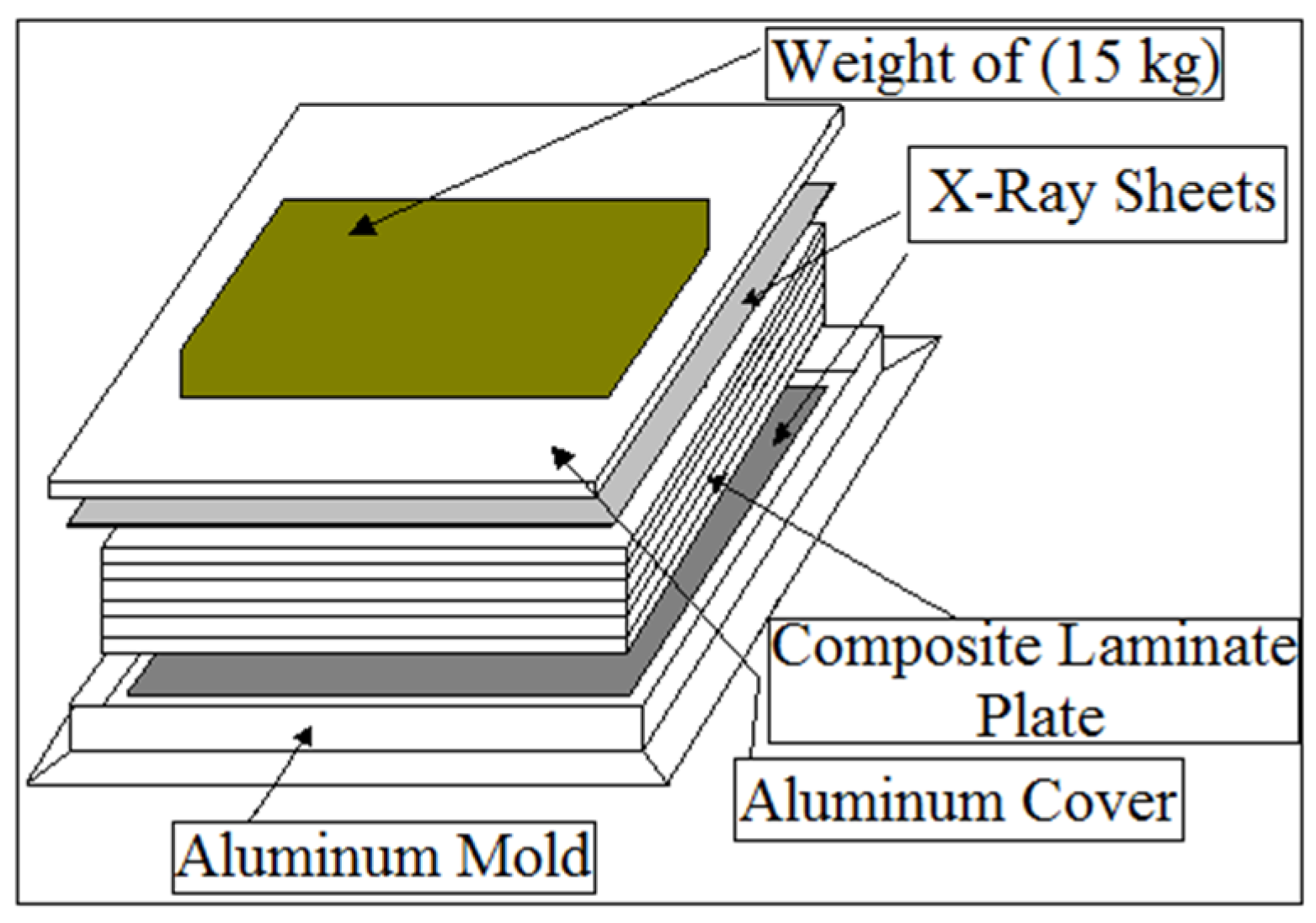
In this study, the fabrication of composite material is consisted of plane E-glass fiber plies in a thermosetting polyester resin. The composite laminate plate is manufactured by hand in the lay-up technique. The fabrication of composite laminates is conducted from six layers of E-glass fabric sheets. The fabric sheets are placed in a (24 cm × 24 cm) aluminum mold. Two X-ray photo sheets are used to avoid abrasion in a specimen surface. The fiber volume fraction is determined experimentally for the composites plate from the following relationship [13]:
where:
φ: is the fiber weight fraction.
And
When the composite with the dimensions (24 × 24) gets dried and gets out from the mold, we can weigh the composite plate to determine (). Before fabrication we can weigh the E-glass fiber to find the value of (). Divide () on () to calculate (ψ). By substituting all these values in Equation (1) we can find the value of () as shown in Figure 1.

Figure 1.
Manufacturing of composite laminated plate.
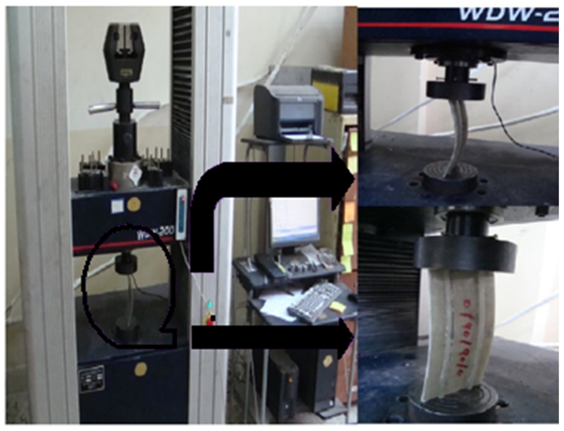
The composite laminated plate with length (200 mm), width (100 mm) and thickness (4 mm) is selected in the experiment test to calculate critical buckling load. One and two stiffeners of width (6 mm) and depth (4 mm) are selected along the length of the main composite plate. The lamination angle for all stiffeners is equal to (0) degrees, while the lamination angle of composite plate is assumed to be cross ply. The dimensions of the specimen that were used in the buckling test has been taken from ASTM E1876 [14]. A tensile test machine was used in a buckling test with an axial compression load of (200 KN) in the vertical direction, as illustrated in Figure 2.
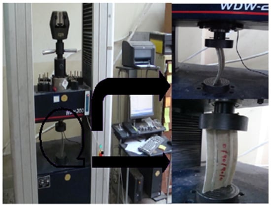
Figure 2.
Buckling test.
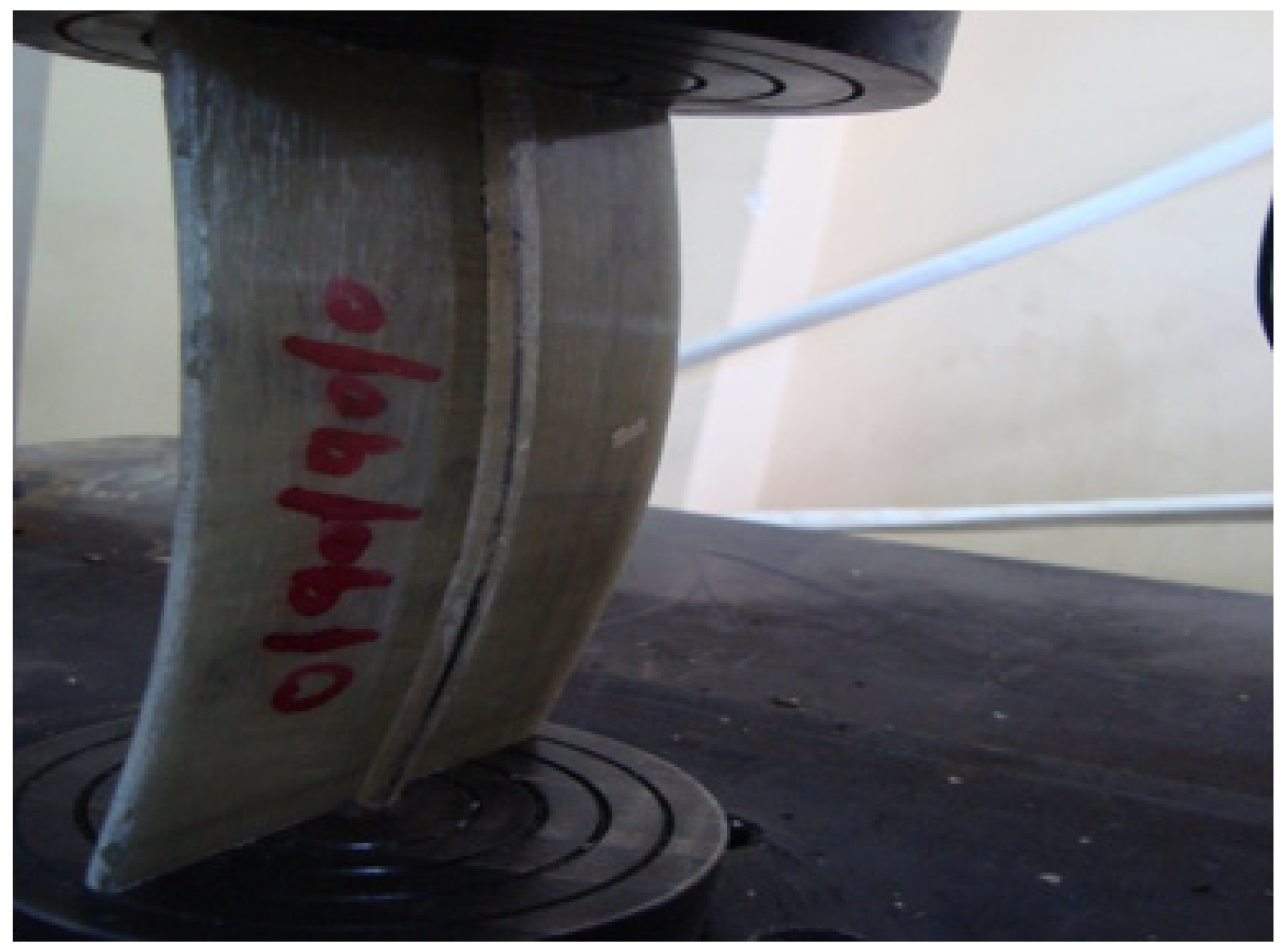
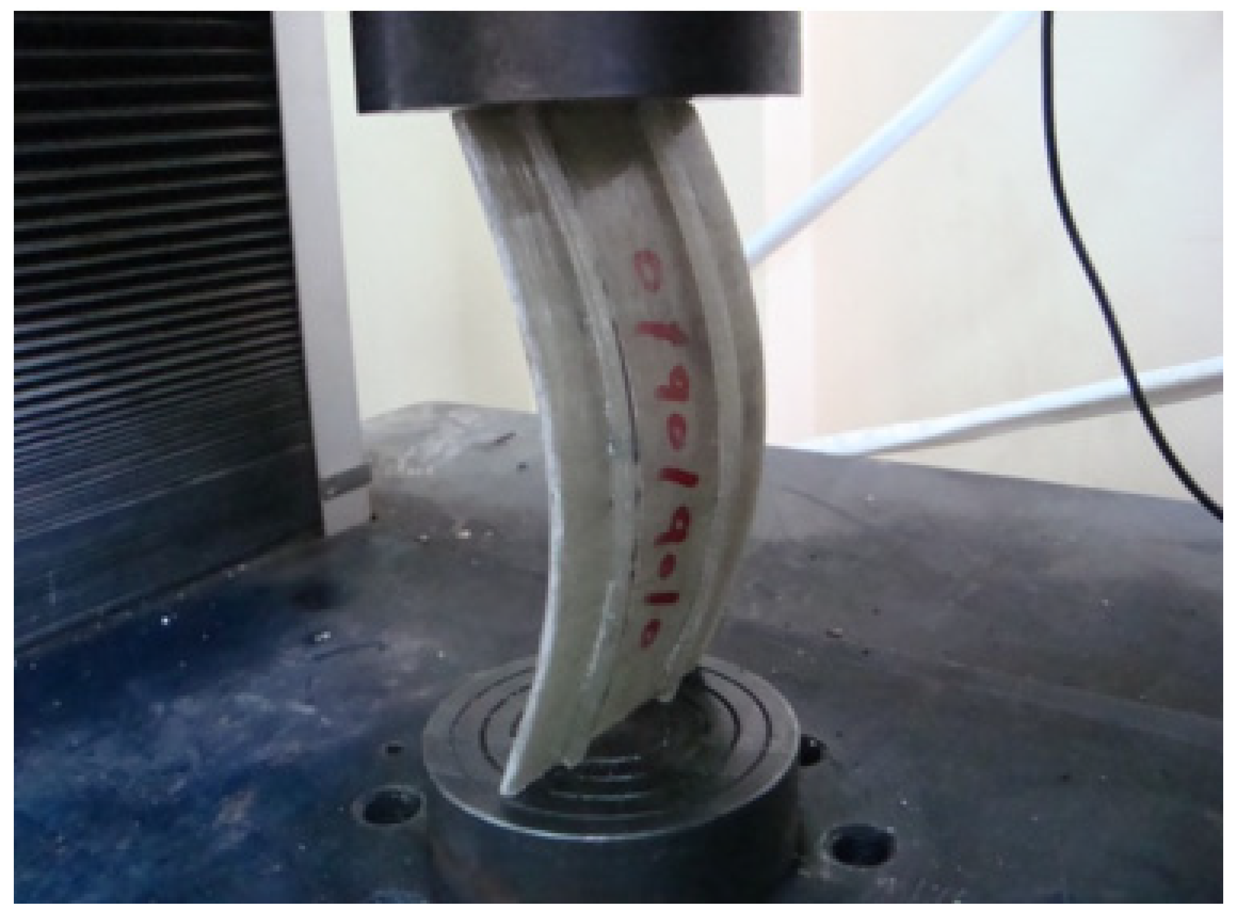
The boundary conditions of the specimen is simply supported by two ends and free at the other two ends (S-F-S-F). The simply supported boundary condition is simulated along the top and bottom edges of the compression test device. The specimen is compressed slowly with a constant cross-head speed of (5 mm/min) until buckling. Figure 3, Figure 4 and Figure 5 show the buckling test for the un-stiffened plate, stiffened plate with one stiffener and stiffened plate with two stiffeners.
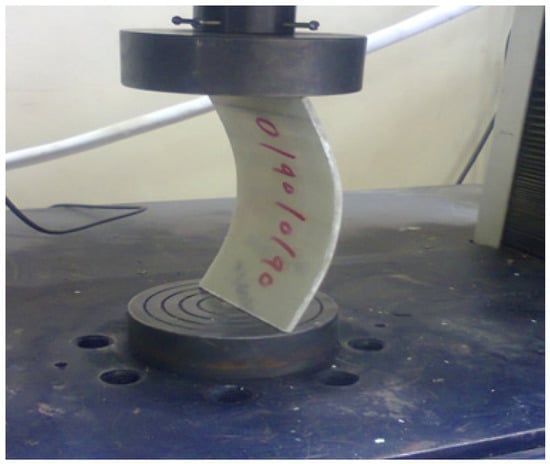
Figure 3.
Buckling test of composite plate without stiffener.
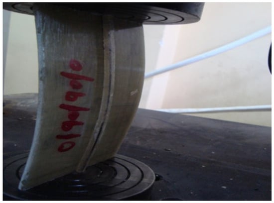
Figure 4.
Buckling test of composite plate with one stiffener.
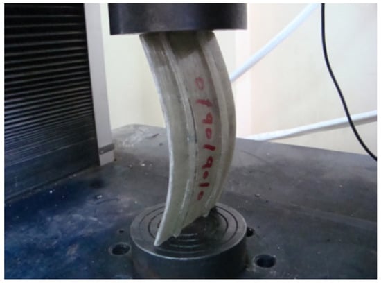
Figure 5.
Buckling test of composite plate with two stiffeners.
For the buckling test loading, the test specimen is placed between two extremely stiff machine heads. The lower head is fixed during the test, whereas the upper one is moved downwards by a servo hydraulic cylinder. The strain gauge is placed in the middle point of the composite laminated plate through the z-axis at the connection point between the composite plate and the stiffener. The strain meter is used to catch the voltage of the bending deflection through the plate thickness due to the in-plane compression mechanical load and the shear force. When the upper head of the servo hydraulic cylinder moves downward, the composite laminated plate will buckle under the effect of the compression load. The data of the bending deflection through the plate thickness against time is stocked in an Excel spreadsheet, and these data were processed using MatLab software. The deflection through the plate thickness is calculated using the following equation:
where:
: is the experiment strain through the composite plate thickness.
: is the experiment bending deflection through the composite plate thickness.
h: is the composite plate thickness.
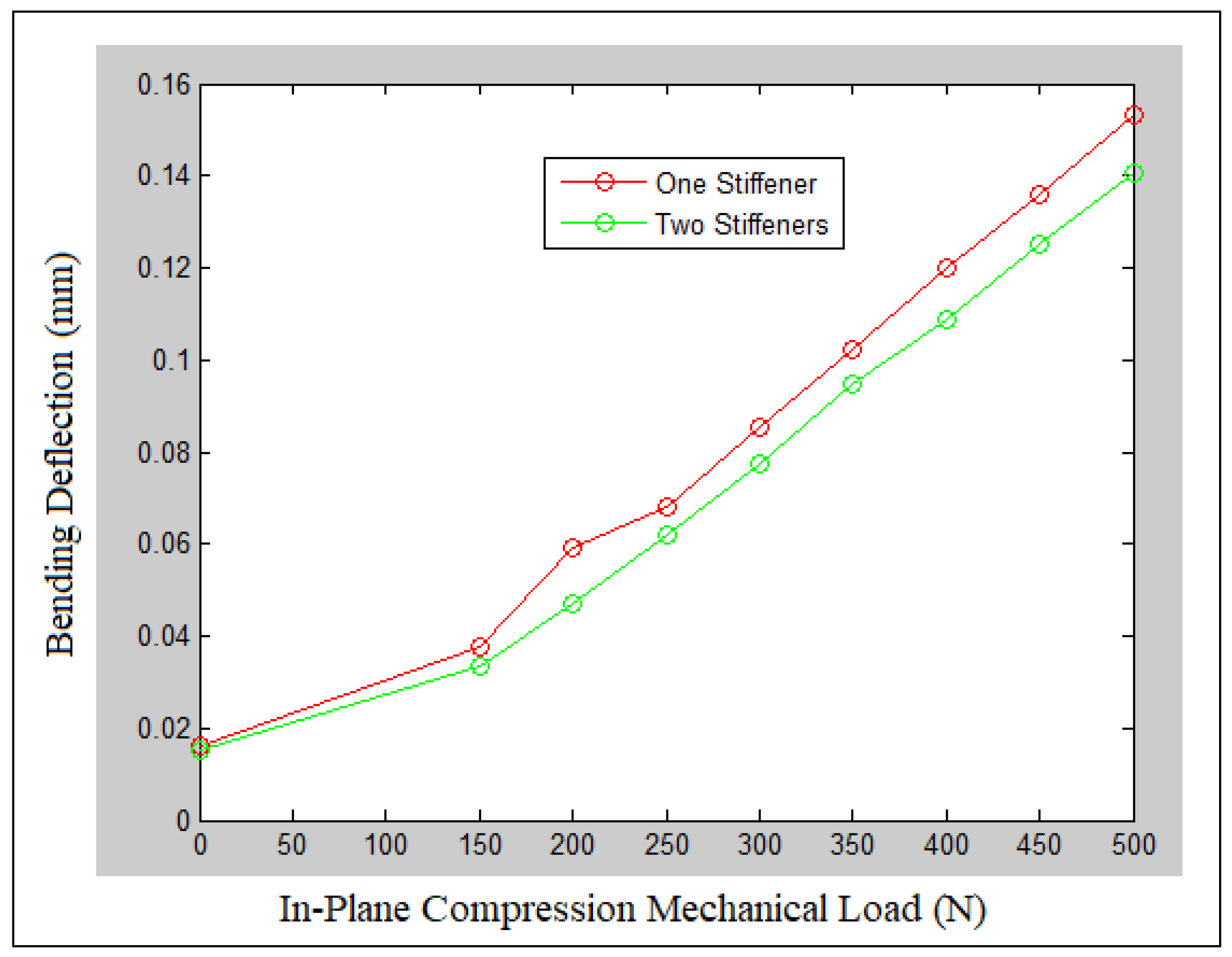
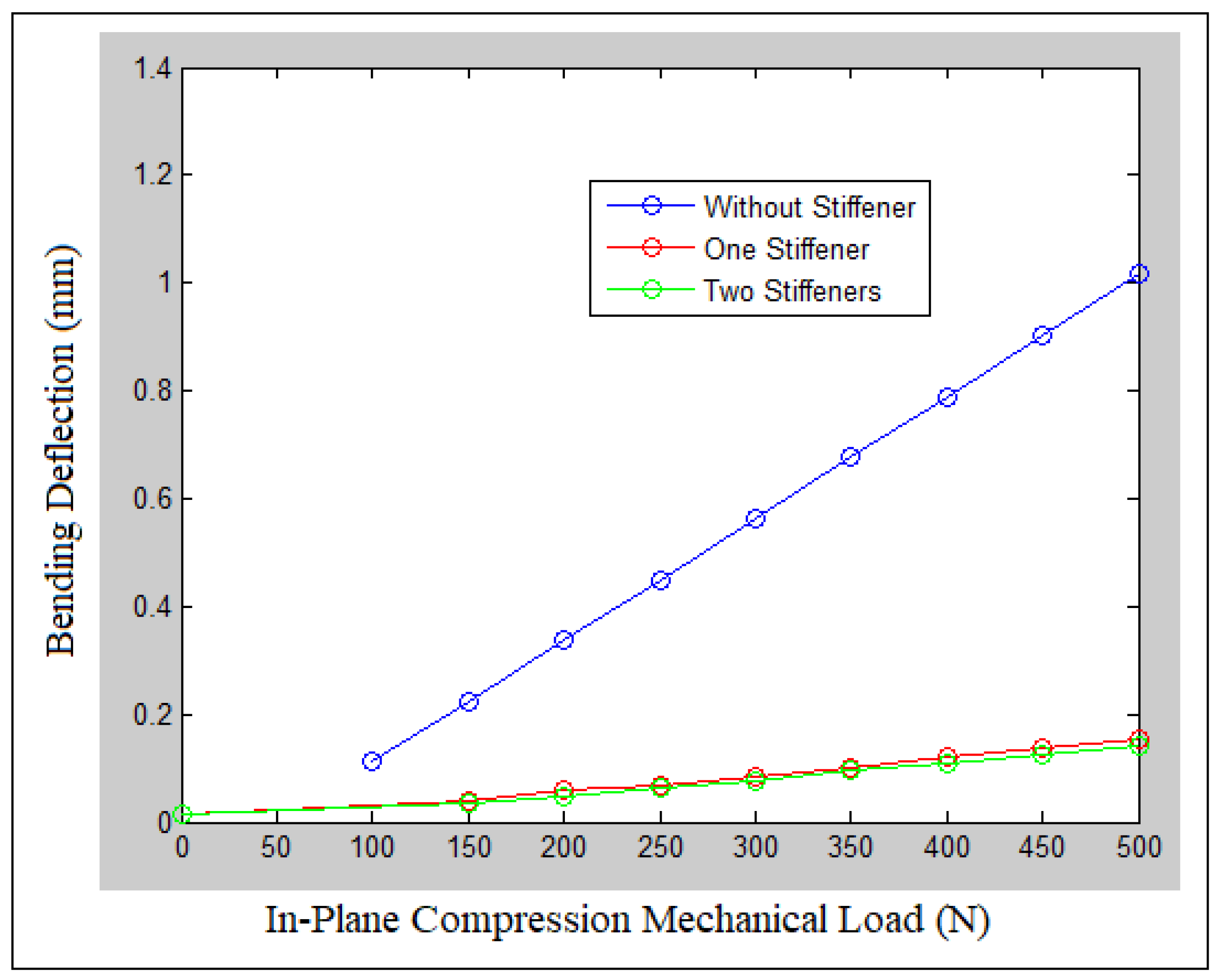
The Southwell plot is a histogram between the bending deflection () and the in-plane compression mechanical load [15]. The in-plane compression mechanical load is readable from the buckling test machine screen since it has the values 100 N, 150 N, 200 N, 250 N, 300 N, 350 N, 400 N, 450 N and 500 N. The relationship between the bending deflection ( and in-plane compression mechanical load is a straight line in which the slop represents the critical buckling load. The Southwell plot is shown in Figure 6 and Figure 7. It can be noticed from Figure 7 that the bending deflection of the un-stiffened and stiffened plates is increased with the increasing of the in-plane compression mechanical load. Moreover, the bending deflection is decreased with the use of beam stiffeners.
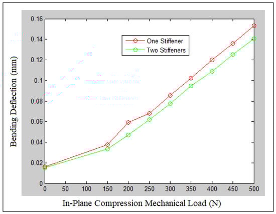
Figure 6.
Bending deflection against in-plane compression mechanical load for plate with one and two stiffeners.
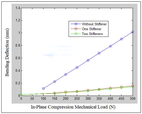
Figure 7.
Bending deflection against in-plane compression mechanical load for un-stiffened plate and plate with one and two stiffeners.
3. Analytic Solution of Bending Deflection
The Levy solution is used in the derivation of bending deflection through plate thickness in which the Levy solution applies to any type of boundary conditions under the effect of in-plane compression mechanical load and shear force. Based on the classical laminate plate theory, the stress–strain relationship is:
where:
Additionally,
The plate equation in terms of bending moments is
The bending moments of the rectangular plate are
where
, since the stacking sequences of plate orientation are the same above and below the z-axis, and this case is called special orthotropic.
Substitute Equation (4) into Equation (3) to obtain the plate equation in terms of the bending stiffness:
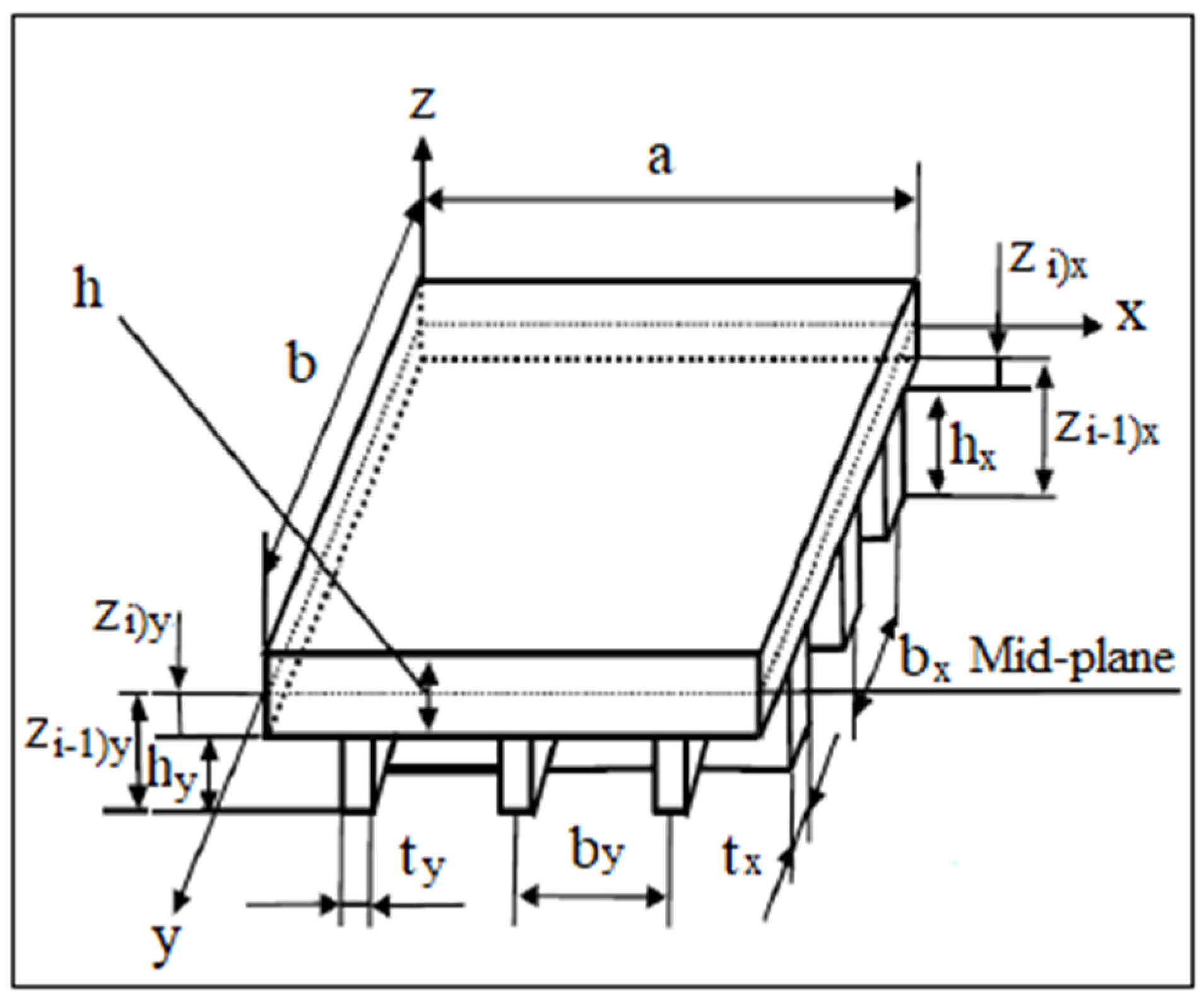
The composite laminated plate with stiffeners is assumed to be orthotropic. The distribution of the beam stiffeners the along (x and y) axis with the dimension is shown in Figure 8.
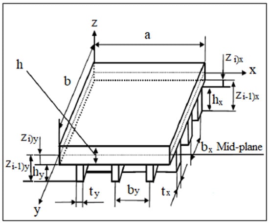
Figure 8.
Distribution of beam stiffeners along (x and y) axis.
The bending stiffness of the composite laminated plate in the presence of the beam stiffeners are:
When the stiffeners are distributed along y-axis,
When the stiffeners are distributed along x-axis,
The solution of Equation (5) is
where
Substitute Equation (6) into Equation (5) to obtain the general solution of the plate equation:
The roots of Equation (7) are
Then
Additionally,
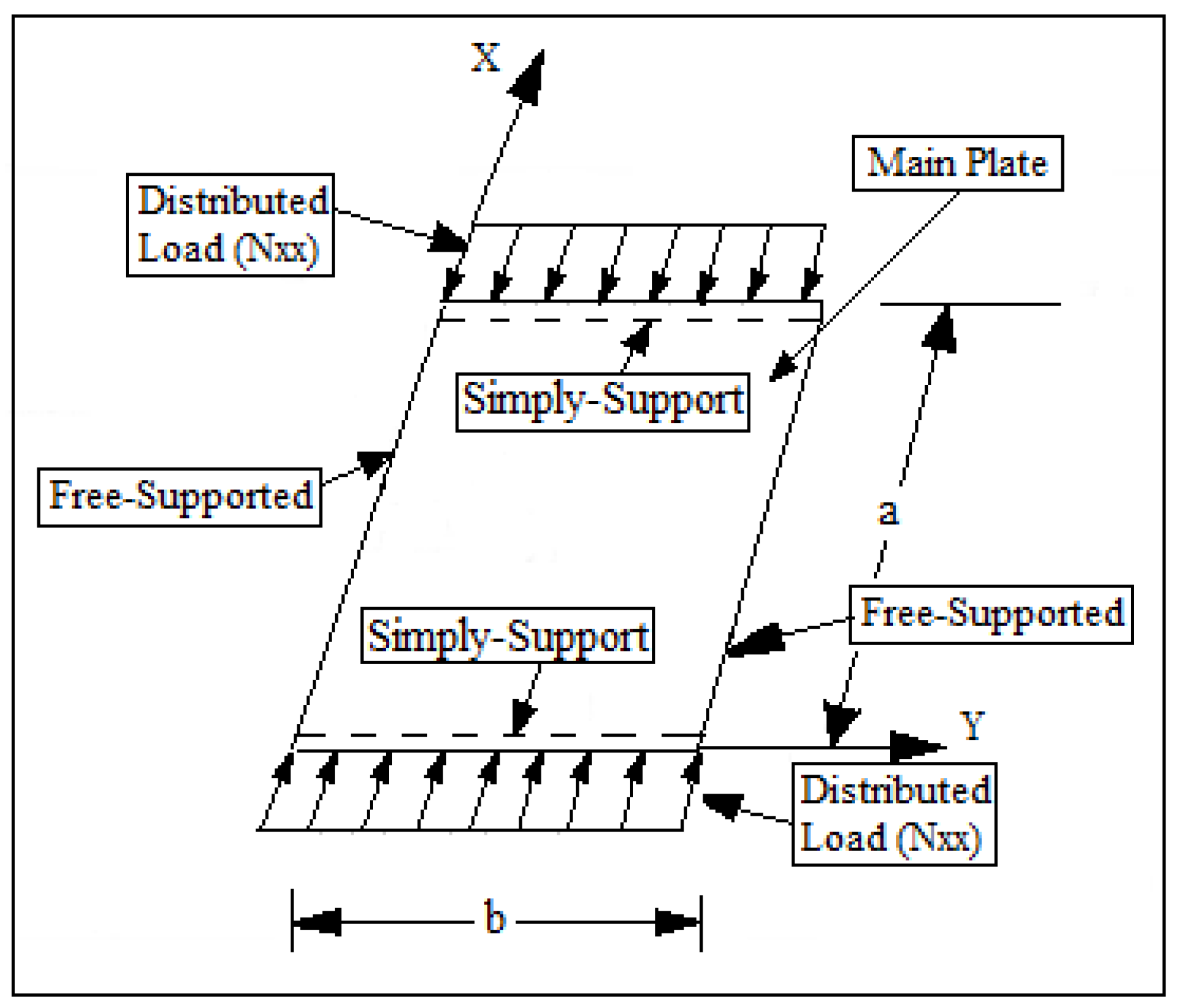
Figure 8 shows the loading and the boundary condition. The Levy solution is assumed that the two sides of the plate are simply-supported boundary conditions along the y-axis, while the x-axis is located in the middle of the plate [5] as shown in Figure 9.
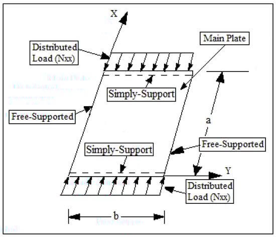
Figure 9.
Loading and the boundary condition of Levy solution.
The bending moments and shear force in terms of the bending stiffness of orthotropic plate are:
As mentioned earlier in experimental section, the boundary conditions are simply supported along the y-axis and free supported along the x-axis. The application of the boundary condition and the solution of bending deflection and critical buckling load can be shown in Appendix A.
5. Different Boundary Conditions
(1) The free–free boundary conditions along the x-axis are assumed to be clamped–clamped while the top and bottom edges of the compression test device stayed simply-supported (S-C-S-C).
B.C. (a) At y = 0, ,
B.C. (b) At y = b, ,
(2) The free–free boundary conditions along the x-axis are assumed to be clamped–simply supported while the top and bottom edges of the compression test device stayed simply supported (S-C-S-S).
B.C. (a) At y = 0, ,
B.C. (b) At y = b, ,
(3) The free–free boundary conditions along x-axis are assumed to be free-clamped while the top and bottom edges of the compression test device stayed simply-supported (S-F-S-C).
B.C. (a) At y = 0, ,
B.C. (b) At y = b, ,
(4) The free–free boundary conditions along x-axis are assumed to be free-simply supported while the top and bottom edges of the compression test device stayed simply-supported (S-F-S-S).
B.C. (a) At y = 0, ,
B.C. (b) At y = b, ,
The constants (A, B, C, D, E, F, G, H, I, J, K, L and M) and , and ) are shown in Appendix B.
6. Numerical Simulation
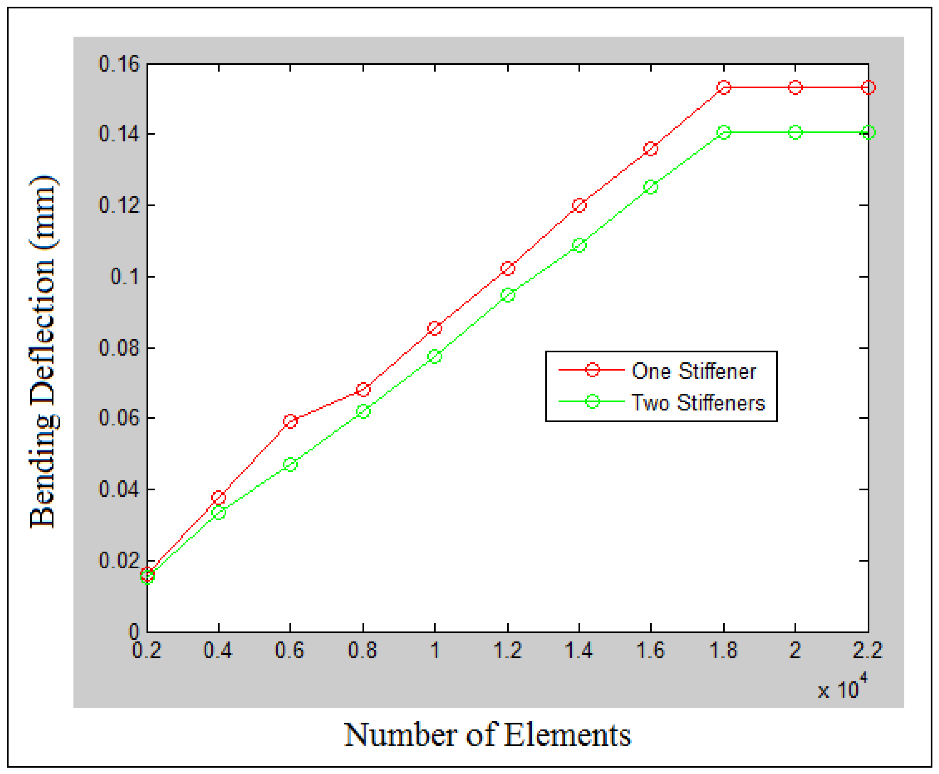
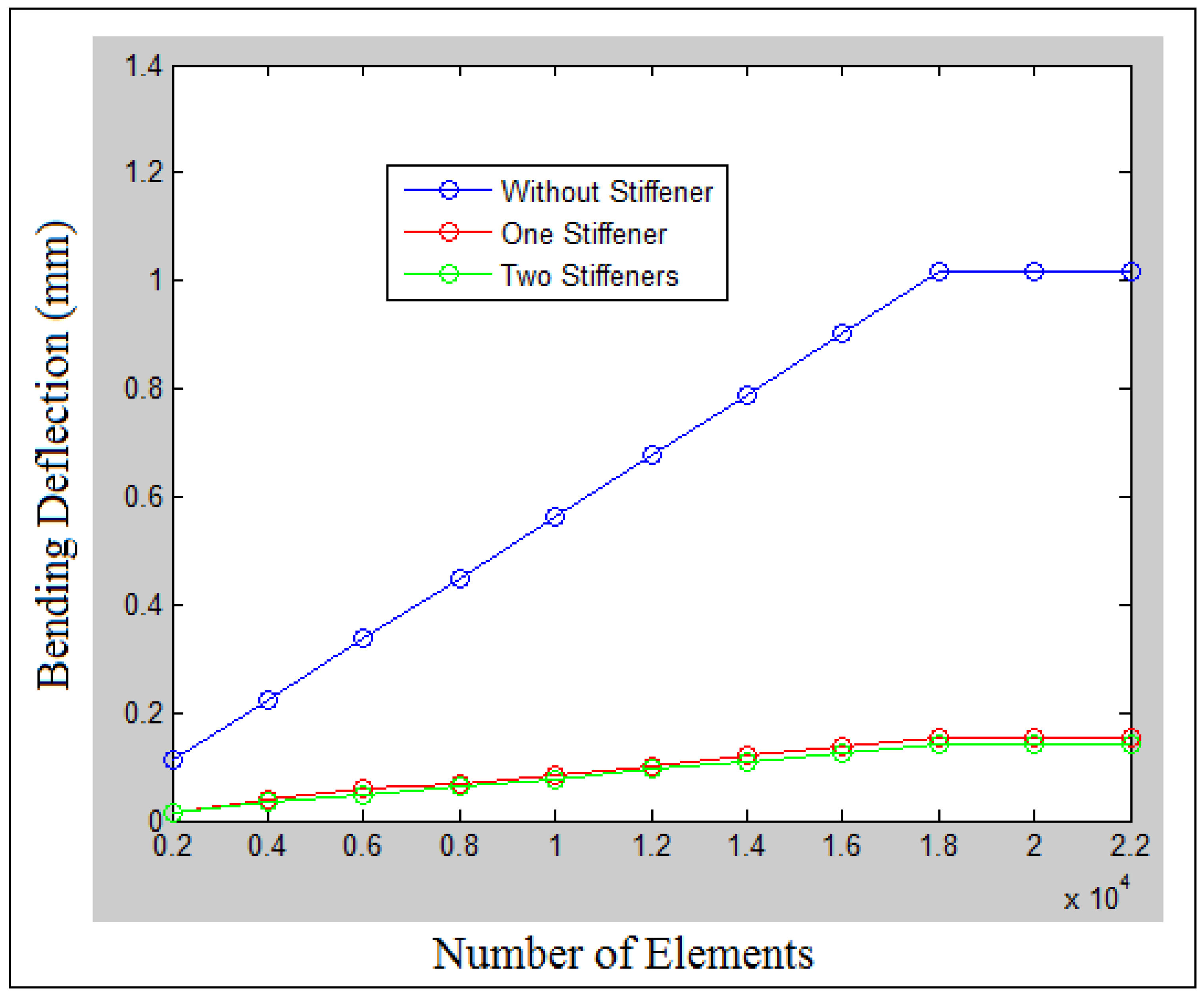
In this paper, the finite element analysis is carried out by using ANSYS [16]. An element (SHELL 99) is selected for the main plate in which this element works with thin and thick plate-shell structures. The element (SHELL 99) has eight nodes with six degrees of freedom at each node; translations in the (x, y and z) axes and rotations about the (x, y and z) axes. This kind of elements used for layered applications for modeling composite plates and shells includes already the effect of transverse shear deformation. For the stiffened plate, the element (SOLSH 190) is used in the simulation, which is having eight nodes connectivity with three degrees of freedom at each node: translations in the nodal (x, y and z) directions. Another three degrees of freedom (rotation) has been added at each node in the nodal (x, y and z) directions. A first order shear deformation theory with the aid of Mindlin–Reissner of shell theory is used by ANSYS software. The global (x) coordinate is directed along the width of the plate, while the global (y) coordinate is directed along the length. The global (z) coordinate corresponds to the thickness direction, which is taken to be outward normal of the plate surface, as shown in Figure 8. For the contact analysis between the main plate and the stiffener, the element (TARGE 170) and the element (CONTA 174) have been used to create the mesh between the target and the contact surfaces. The stiffener represents the target, while the main plate is the source. The mesh generation for un-stiffened plates, stiffened plates with one stiffener and stiffened plates with two stiffeners are illustrated in Figure 10, Figure 11 and Figure 12. The convergence test is completed using a high number of elements to determine the exact size of the element when the value of bending deflection is settled down, as indicated in Figure 13 and Figure 14.
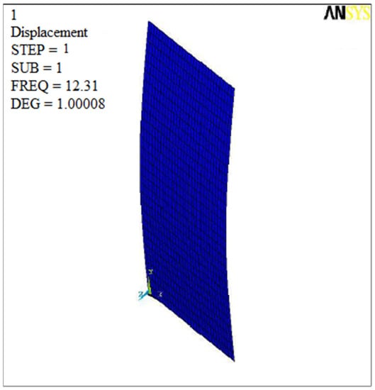
Figure 10.
Mesh contour of composite laminated plate without stiffener.
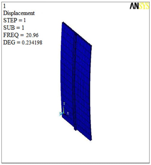
Figure 11.
Mesh contour for composite laminated plate with one stiffener.

Figure 12.
Mesh contour for composite laminated plate with two stiffeners.
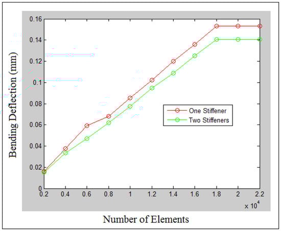
Figure 13.
Convergence test of bending deflection against number of elements for plate with one and two stiffeners.
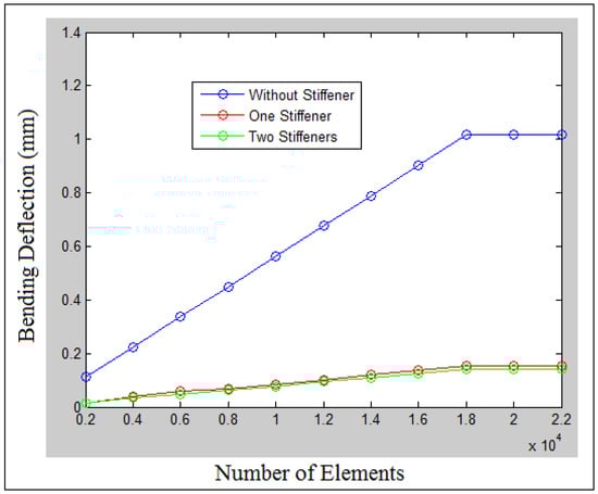
Figure 14.
Convergence test of bending deflection against numbers of elements for plate with and without stiffeners.
7. Largest Lyapunov Exponent Parameter
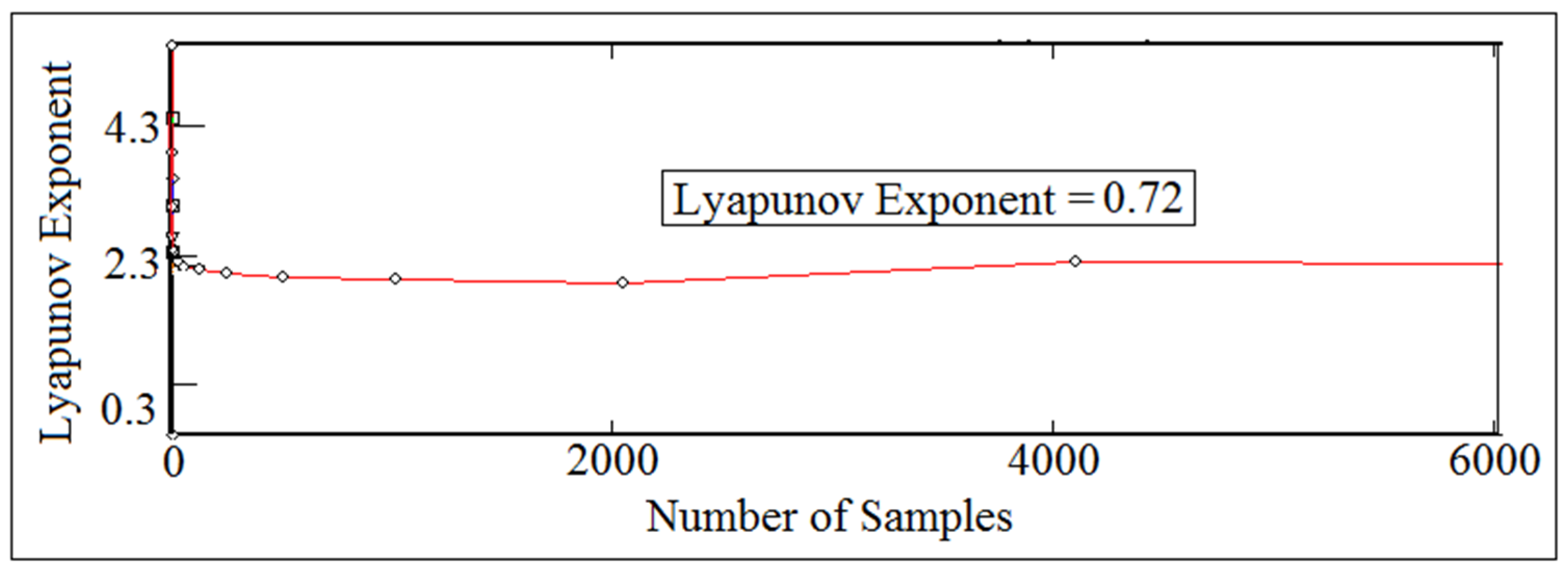
In the design, the largest Lyapunov exponent parameter is one of the indicators to detect the non-periodic motion and chaos of the bending deflection of the stiffened composite laminated plate. The higher the value of the Lyapunov exponent parameter, the more non-periodic the motion and chaos. The value of the Lyapunov exponent of the bending deflection being positive means that the motion of the bending deflection is non-periodic. The negative largest Lyapunov exponent value of the bending deflection indicates periodic motion. The Wolff algorithm code based on MATLABB software is used to extract the values of the largest Lyapunov exponent by monitoring the orbital divergence for the contact force [17]. Equations (19) and (20) were used to build the Wolff algorithm code of the dynamic tool [18].
Figure 15 shows the numerical value of the largest Lyapunov exponent against the number of samples at a fiber volume fraction (80%) and aspect ratio (2.5) for an un-stiffened composite laminated plate. The value of the Lyapunov exponent parameter is taken at its respective equilibrium point. One column of the bending deflection with the values of time delay and embedding dimension are used in the Wolff algorithm to extract the numerical value of the largest Lyapunov exponent parameter. One column of the bending deflection has been taken from the ANSYS program, in which it used the dynamic tool of the Wolff algorithm code.
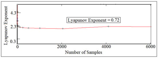
Figure 15.
Local Lyapunov exponent against number of samples for ( = 80%) and (a/b = 2.5).
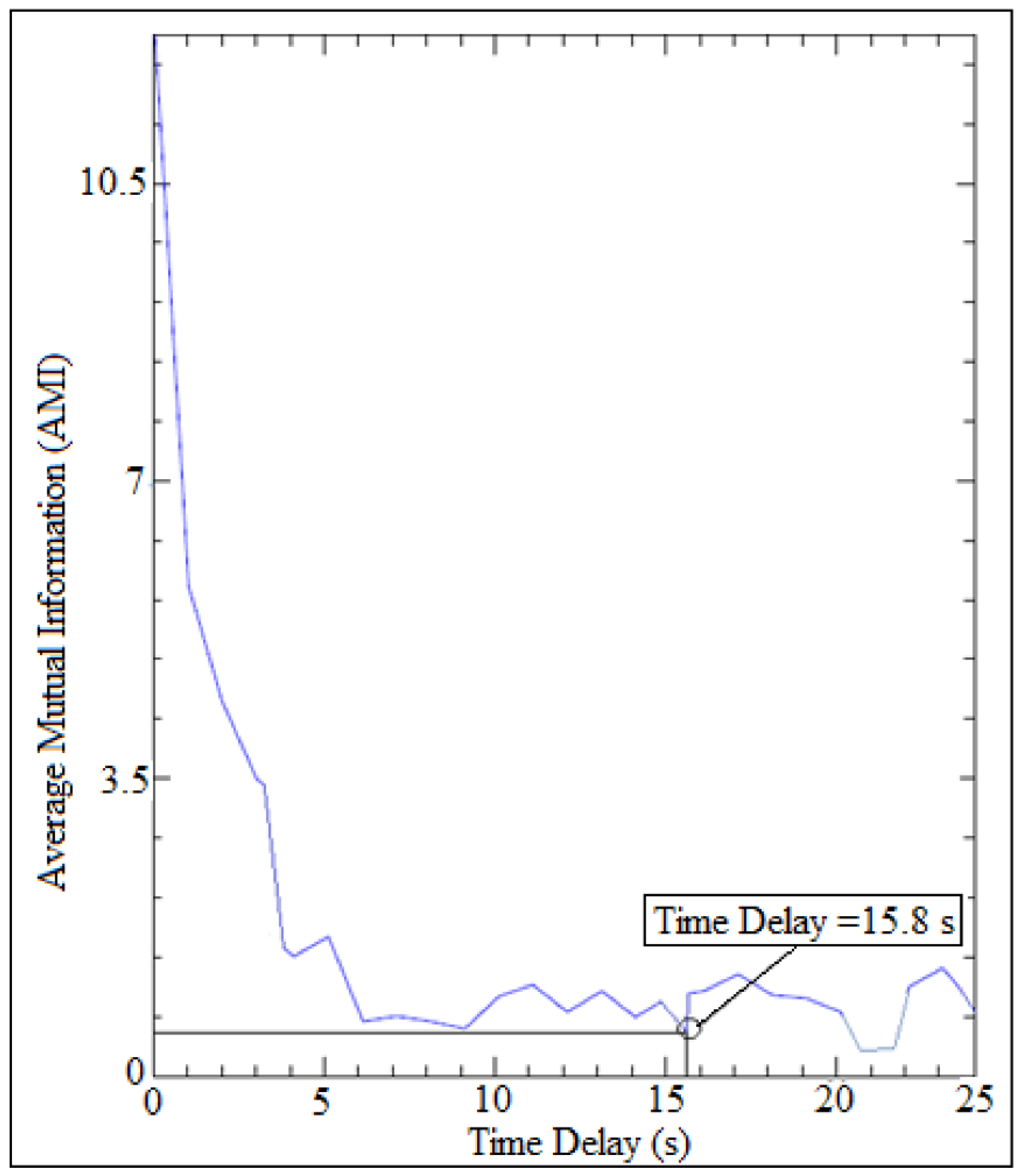
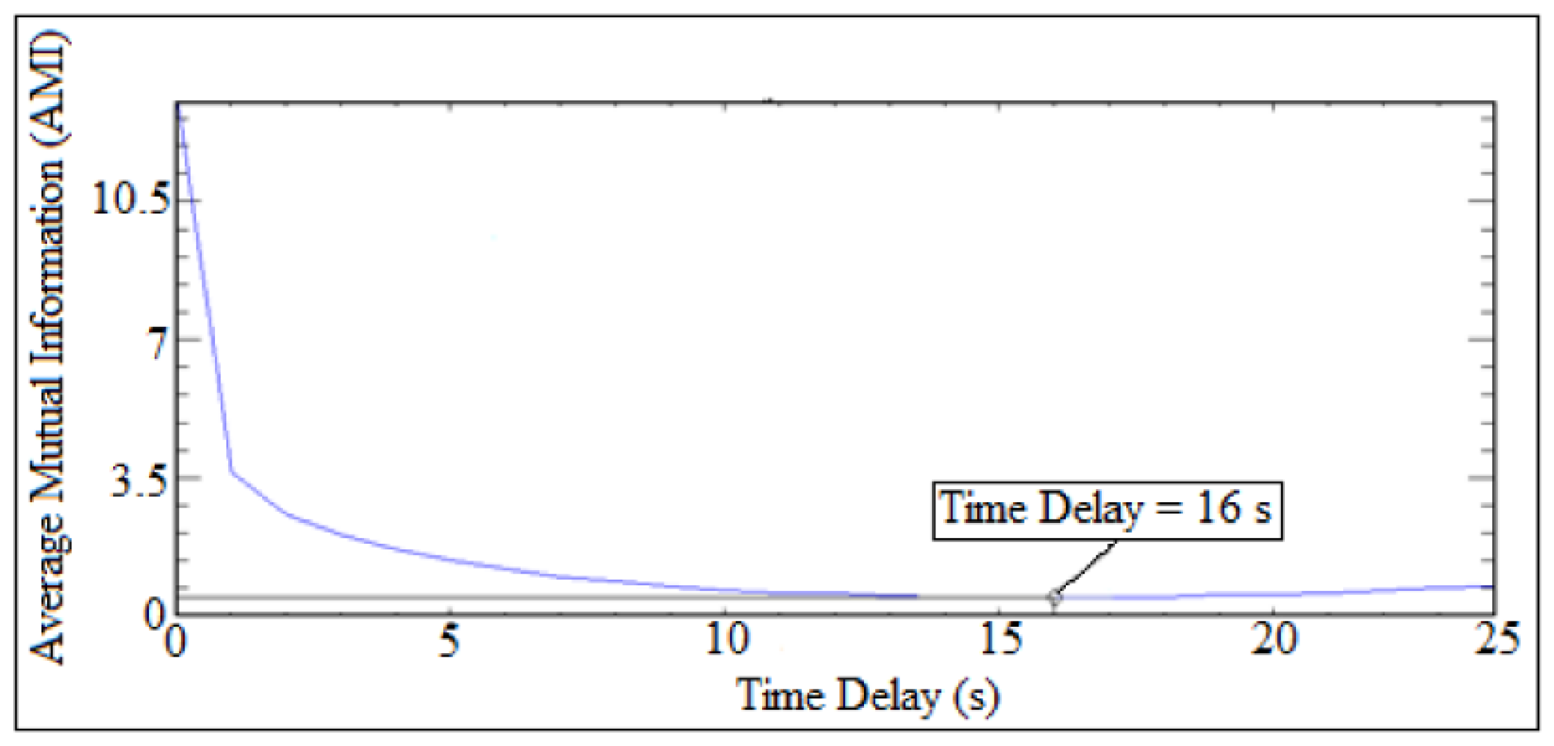
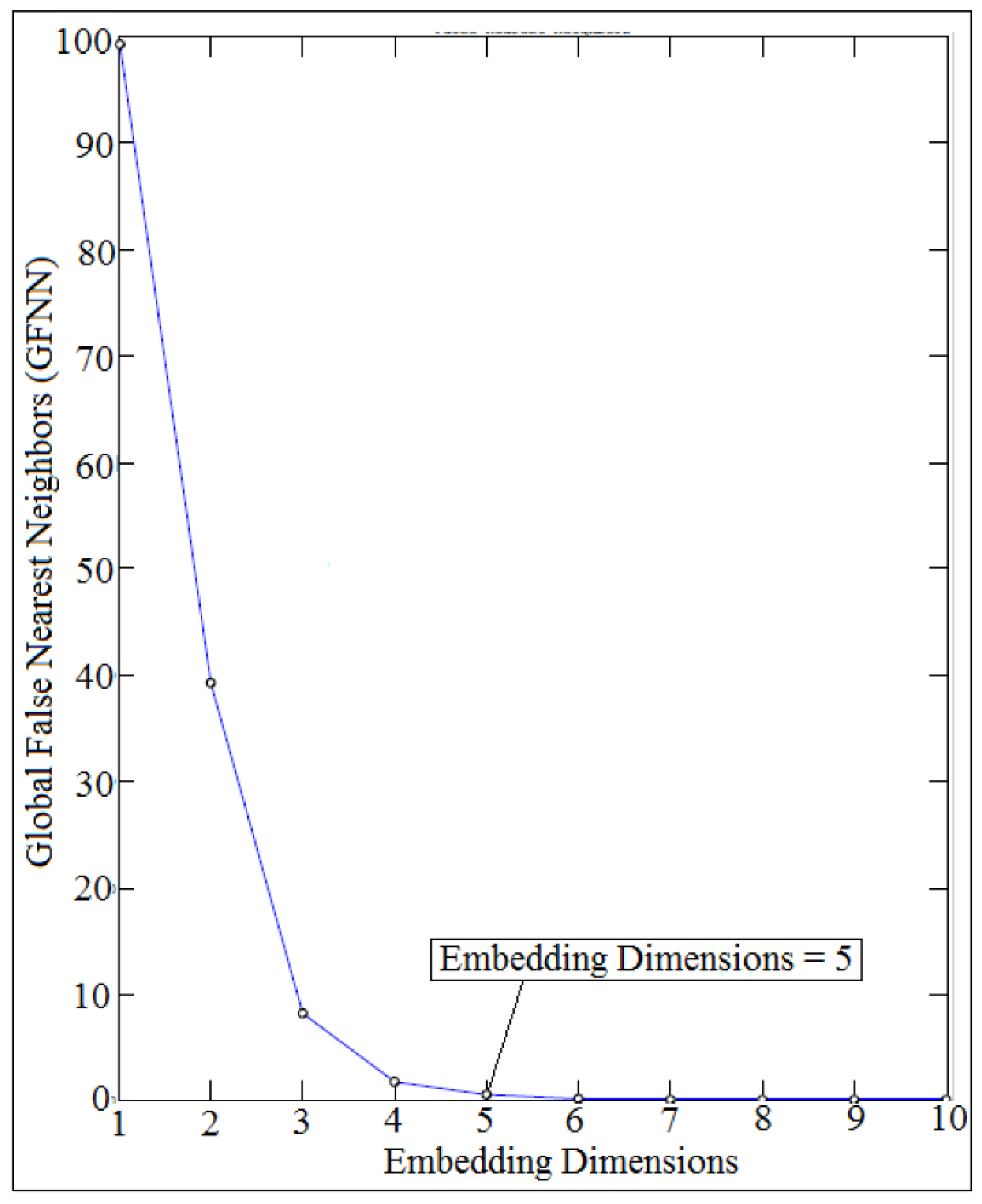
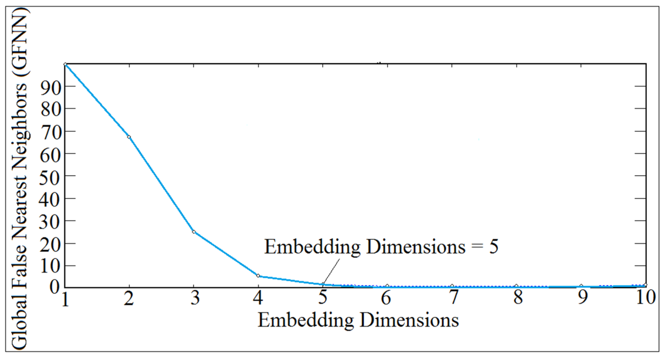
Time delay and embedding dimensions are numeric values in which it is needed in the Wolff algorithm code in the estimation of the local Lyapunov exponent parameter. The algorithm of the dynamic code of the global false nearest neighbors (GFNN) of the bending deflection is used to obtain the value of the embedding dimensions, in which it is estimated when the trend of global false nearest neighbors approaches zero [19]. In this paper, a local and optimal time delay was estimated in which it is recommended that the local time delay should be chosen to be dependent on the embedding dimensions [20]. The algorithm code of the average mutual information (AMI) is used to obtain the value of the time delay, and the first minimum time in the average mutual information trend represents the value of the time delay. The optimal time delay is calculated from the following equation:
where
: is the local time delay.
: is the optimal for independence of time series.
P: is the embedding dimensions.
Figure 16 and Figure 17 show the comparison of time delay, while Figure 18 and Figure 19 show the comparison of embedding dimensions.
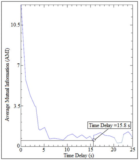
Figure 16.
Time delay of numerical simulation.
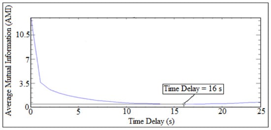
Figure 17.
Time delay of experiment test.
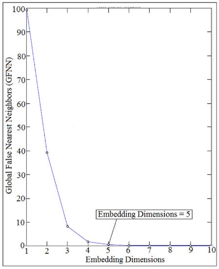
Figure 18.
Embedding dimensions of numerical simulation.
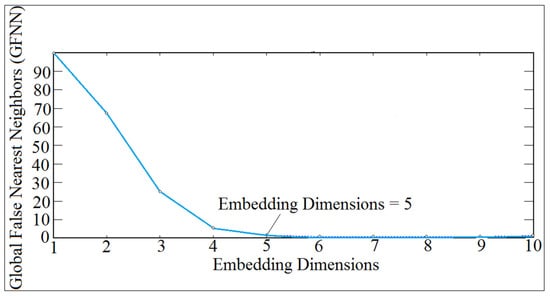
Figure 19.
Embedding dimensions of experiment test.
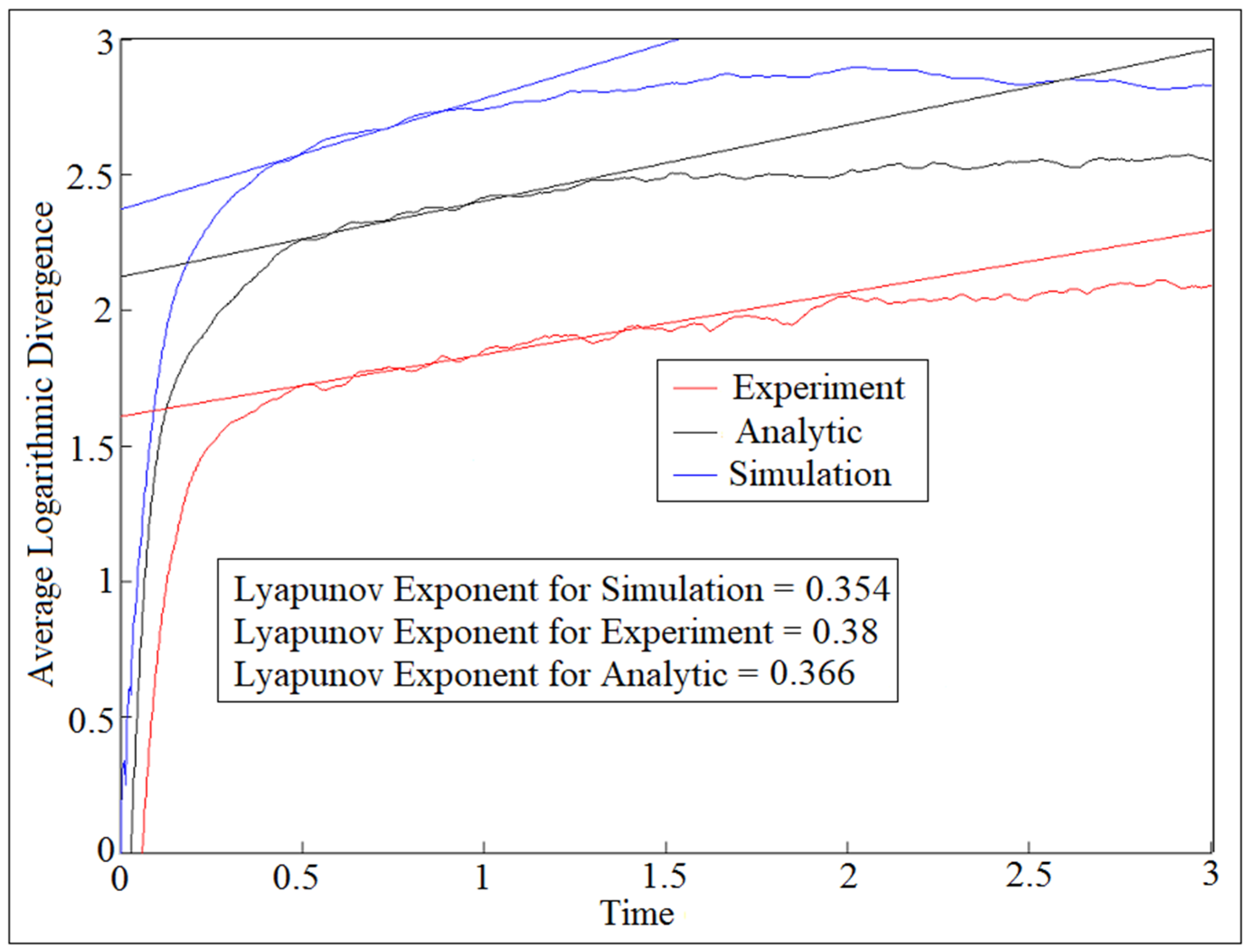
There is another way for estimating the largest Lyapunov exponent of the bending deflection that is called the average logarithmic divergence. The straight line represents the slope of the average logarithmic divergence, which reflects the value of the Lyapunov exponent parameter. The curve represents the logarithm function against time of the bending deflection. As known, the logarithm function treats any set of data by a straight line, which gives the value of the largest Lyapunov exponent directly. Figure 20 shows the comparison of the average logarithmic divergence of bending deflection against time at a fiber volume fraction (80%) and aspect ratio (2.5) for a plate with two stiffeners. The analytic largest Lyapunov exponent of the bending deflection is calculated after applying Equation (9) on one column of the bending deflection using the average logarithmic divergence approach, while the numerical simulation of the largest Lyapunov exponent of the bending deflection is determined using the ANSYS program. The experiment value of the largest Lyapunov exponent has been obtained after tracking the bending deflection in the direction of the plate thickness using the strain gauge through the strain meter.
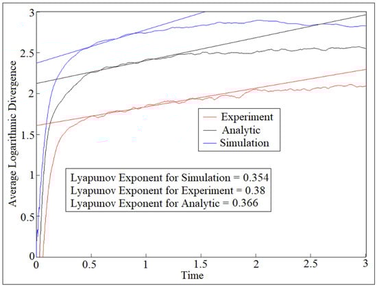
Figure 20.
Average logarithmic divergence against the time for ( = 80%) and (a/b = 2.5).
8. Power Density Function of Fast Fourier Transfer (FFT)
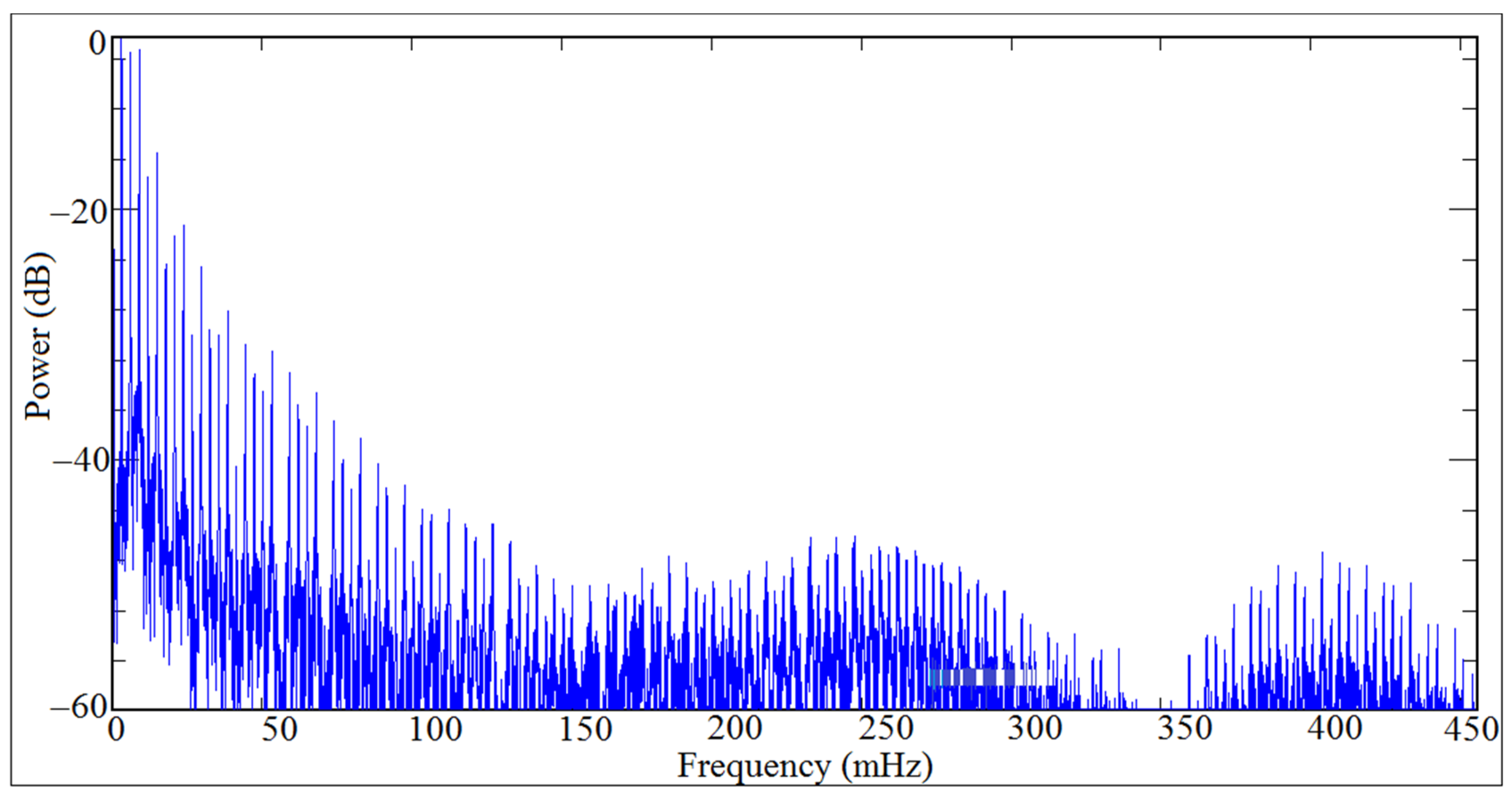
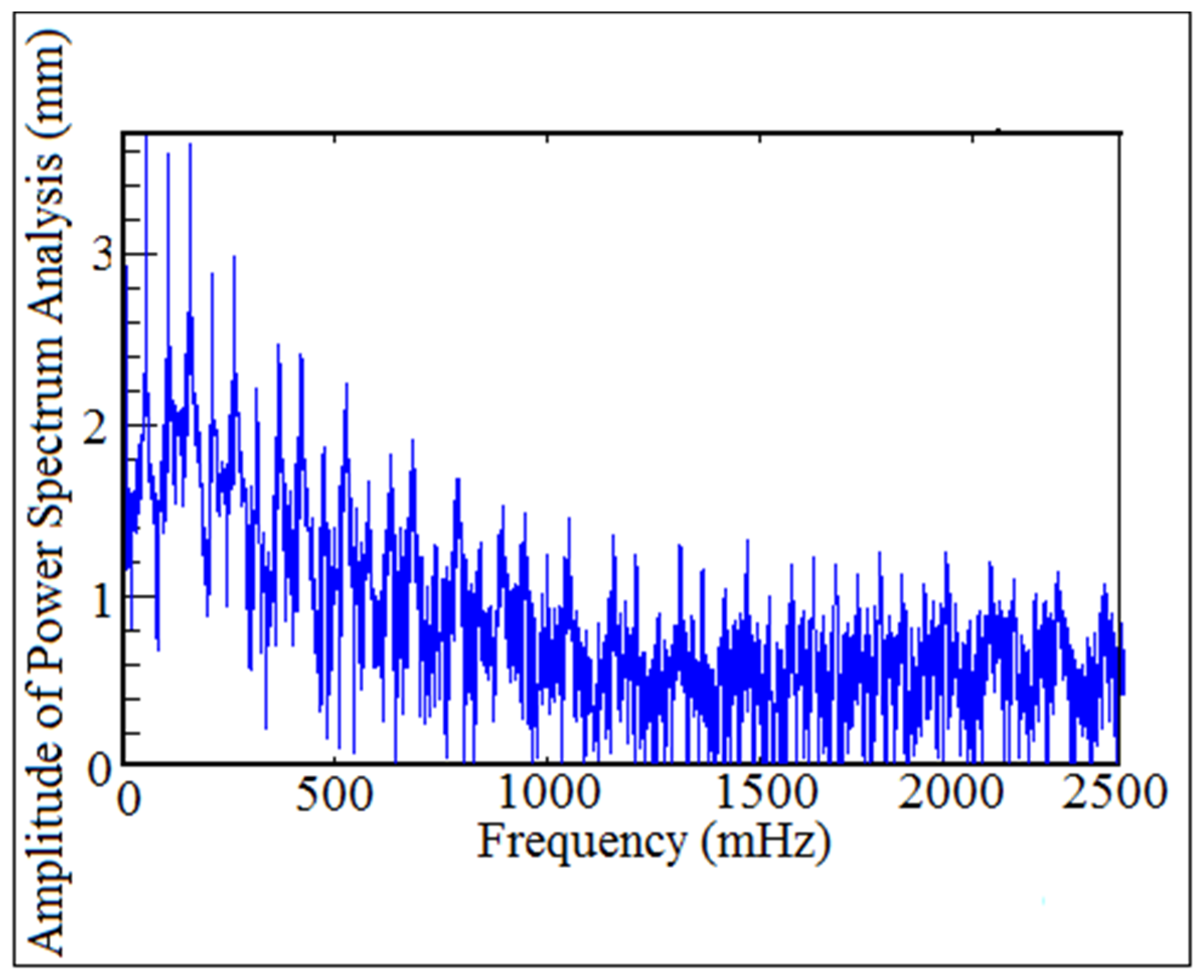
Power density function is used to detect the non-periodic motion and chaos of the bending deflection of the stiffened composite laminated plate since it gives six frequencies peaks’ alongside the fundamental frequency [21]. The signal power is the most important factor for signal quality, in which the noise can be measured by using the indicator SNR ratio. SNR is the ratio between the wanted signal and the unwanted noise. When the SNR of the bending deflection signal has a maximum value, it means that there is no error or noise in the bending deflection signal. The SNR power of the bending deflection signal is measured by the dB scale since it could be either positive or negative. A negative SNR means that the signal power is lower than the noise power. When the power of the amplitude peak of the fundamental frequency and the other frequencies are decreased with the increasing of number of samples, it means that the motion of the bending deflection is non-periodic motion and chaos. When the frequencies’ peaks have not been started disappearing from (FFT) diagram, the motion of the bending deflection is quasi-periodic. Figure 21 and Figure 22 show the comparison of the power density function of the fast Fourier transform (FFT) of the bending deflection at the fiber volume fraction (25%) and aspect ratio (2.5) for the un-stiffened plate. The SNR of the bending deflection signal is positive and equal to (17.24 dB).
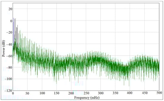
Figure 21.
Power spectrum analysis of the experiment test of the bending deflection for ( = 25%) and (a/b = 2.5).
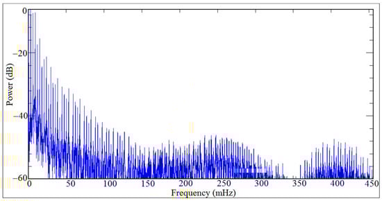
Figure 22.
Power spectrum analysis of the numerical simulation of the bending deflection for ( = 25%) and (a/b = 2.5).
9. Results and Discussion
Table 1 shows the comparison of the critical buckling load of (S-F-S-F) boundary conditions for different orientations when the plate is stiffened with one and two stiffeners. The critical buckling load is increased with the increasing of orientations and number of stiffeners. The critical buckling load results at the orientations (0/90/0/90) and (0/90/90/0) and are the same when the main plate is stiffened by one stiffener. When the main plate is stiffened by two stiffeners, the results of critical buckling load are not the same at the orientations (0/90/0/90) and (0/90/90/0). The numerical results of the critical buckling load were done using the ANSYS program while the experiment results were carried out using strain gauge through a strain meter device. The analytic results of the critical buckling load were completed using the Levy solution of classical laminate plate theory.

Table 1.
Comparison of critical buckling load for (S-F-S-F) boundary conditions against fiber orientation for one and two stiffeners.
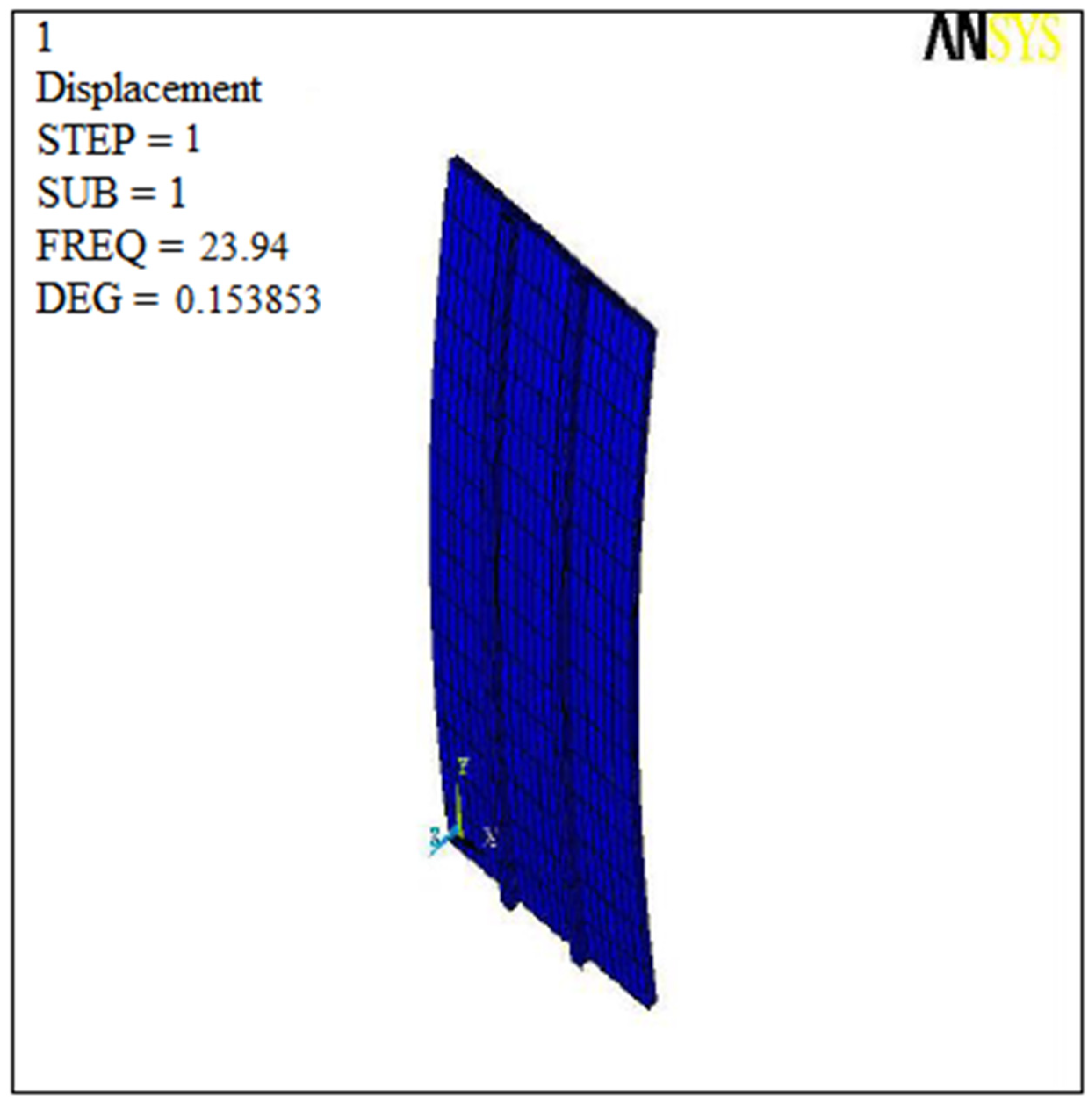
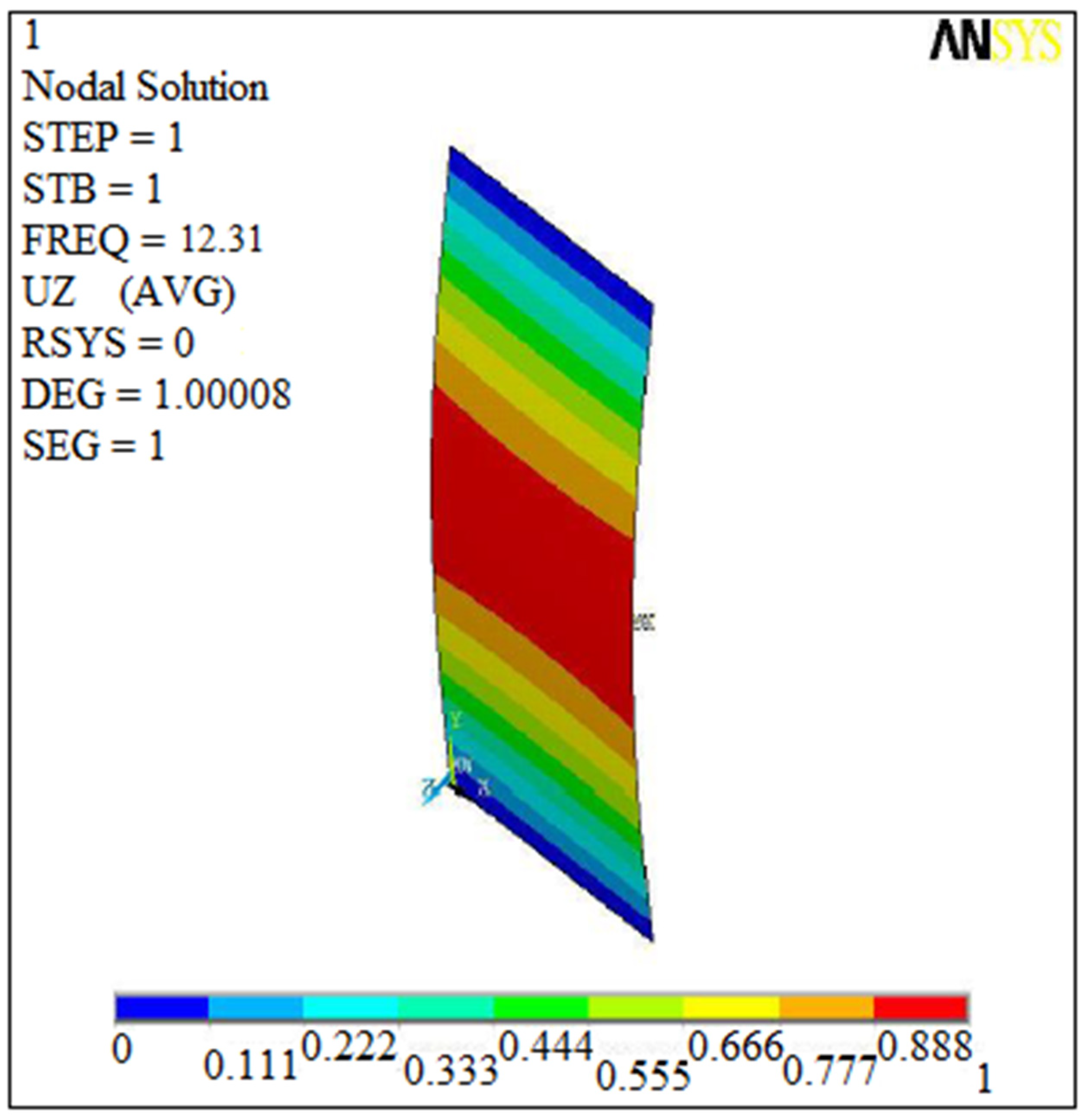
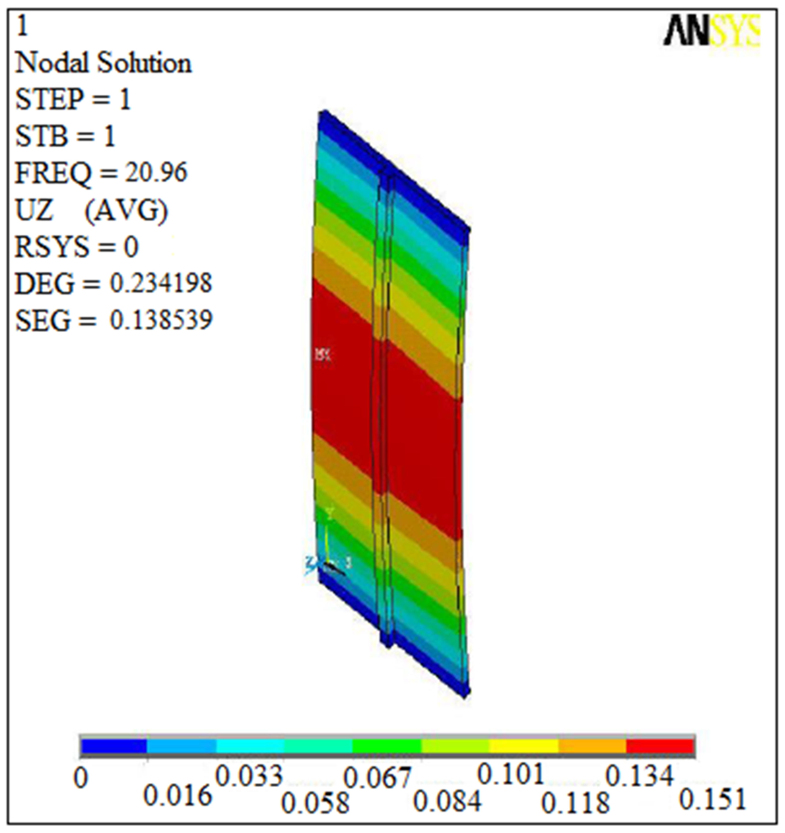
Figure 23, Figure 24 and Figure 25 show the deflection contour distribution for the un-stiffened plate, stiffened plate with one stiffener and stiffened plate with two stiffeners of fiber orientation (0/90). The frequency was 12.31 Hz, 20.96 Hz and 23.94 Hz for the un-stiffened plate, stiffened plate with one stiffener and stiffened plate with two stiffeners, respectively. The central point in the middle of the main plate was considered in the calculation of the bending deflection contour. The maximum bending deflection decreased with the increasing of number of stiffeners. The ANSYS program was used in the calculation of the bending deflection contour.

Figure 23.
Bending deflection contour for un-stiffened plate.
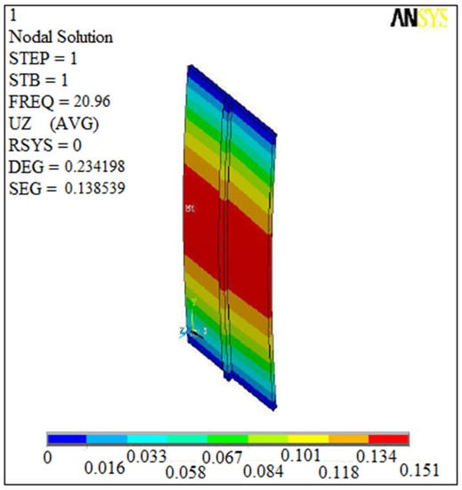
Figure 24.
Bending deflection contour for plate with one stiffener.
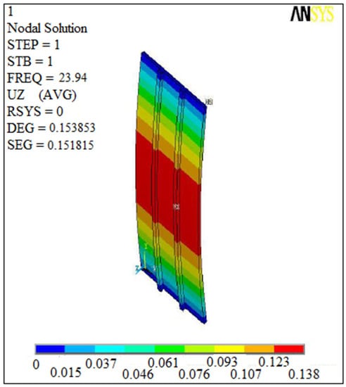
Figure 25.
Bending deflection contour for plate with two stiffeners.
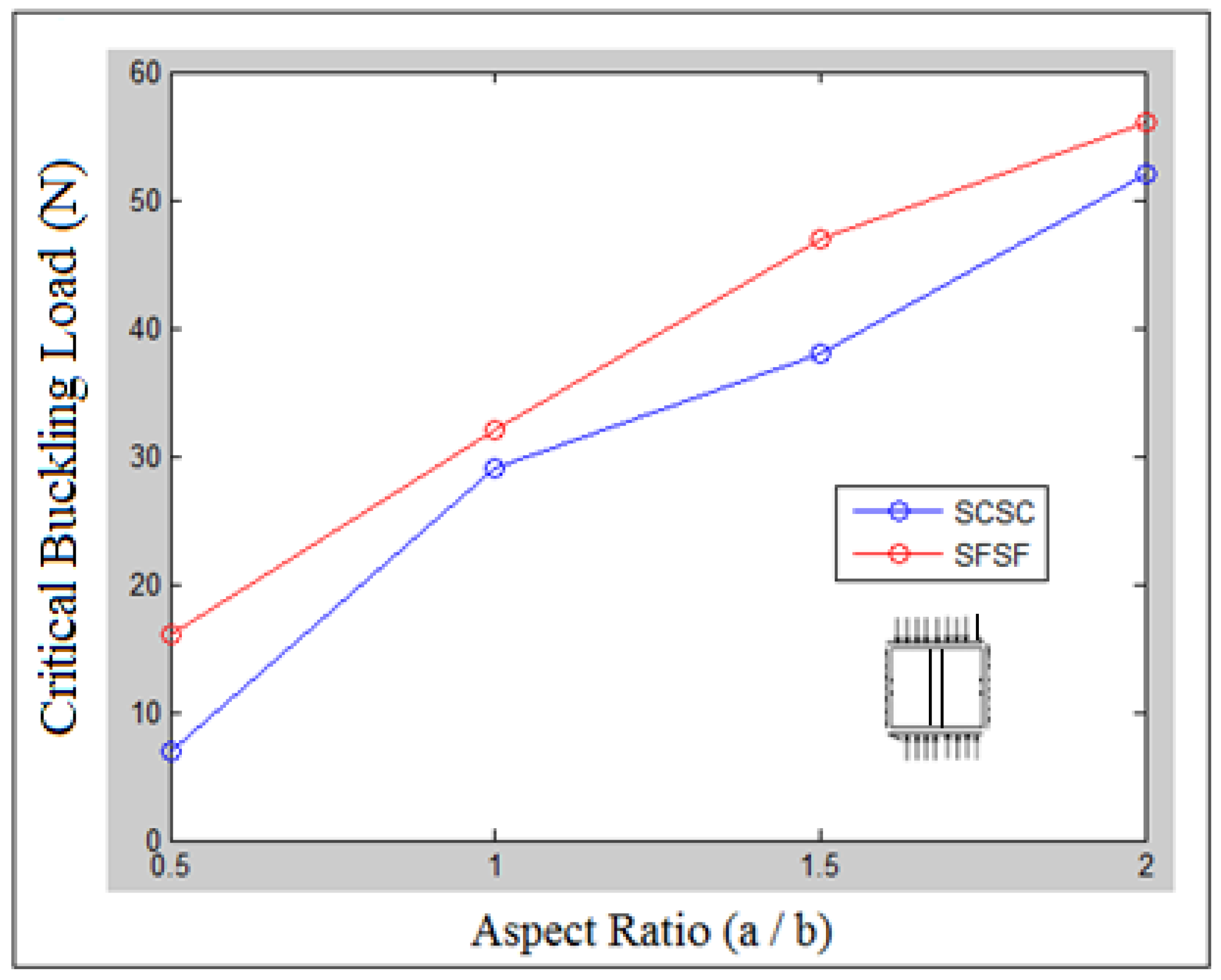
Figure 26 shows the critical buckling load against the aspect ratio of (S-C-S-C and S-F-S-F) boundary conditions for plate with one stiffener in the presence of in-plane compression mechanical load and shear force. The critical buckling load increased with the increasing of the aspect ratio. The critical buckling load value for (S-F-S-F) boundary conditions is greater than the value of the critical buckling load for (S-C-S-C) boundary conditions. The two clamped boundary conditions in (S-C-S-C) generate shear stress in the opposite direction, which reduces the value of critical buckling load. The ANSYS program is used in the calculation of the critical buckling load.
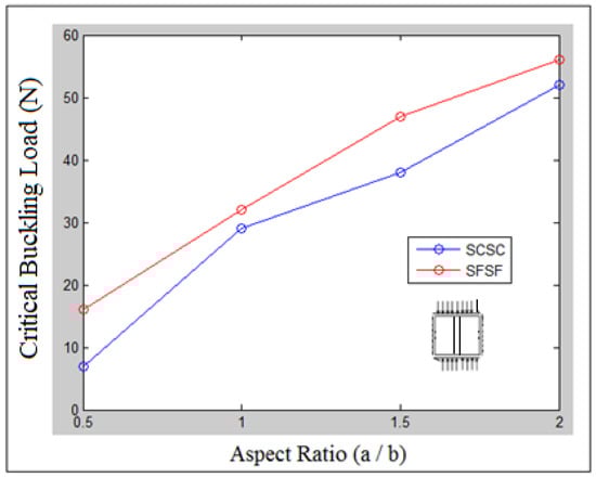
Figure 26.
Critical buckling load against aspect ratio for (S-C-S-C) and (S-F-S-F) boundary conditions.
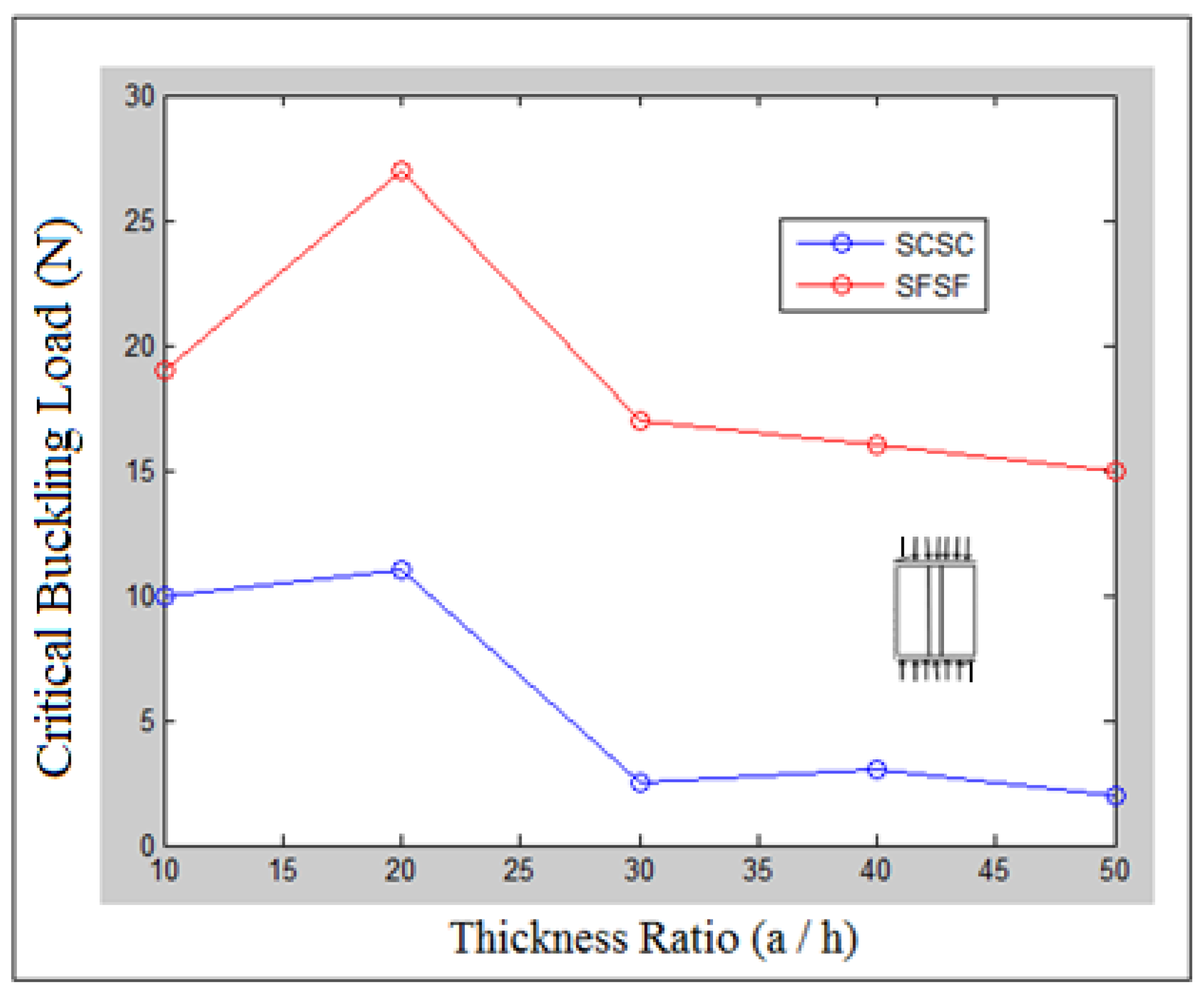
Figure 27 shows the critical buckling load against the thickness ratio for (S-C-S-C and S-F-S-F) boundary conditions for plate with one stiffener in the presence of the in-plane compression mechanical load and shear force. The critical buckling load is varied sinusoidal with a thickness ratio in which it reaches a maximum value at thickness ratio (a/h = 20). The ANSYS program is used in the calculation of the critical buckling load.
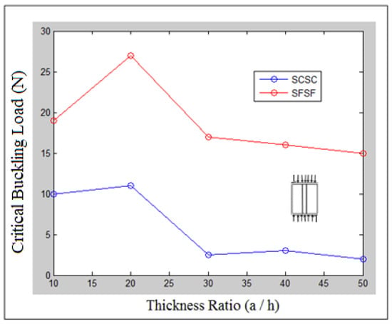
Figure 27.
Critical buckling load against thickness ratio for (S-C-S-C) and (S-F-S-F) boundary conditions.
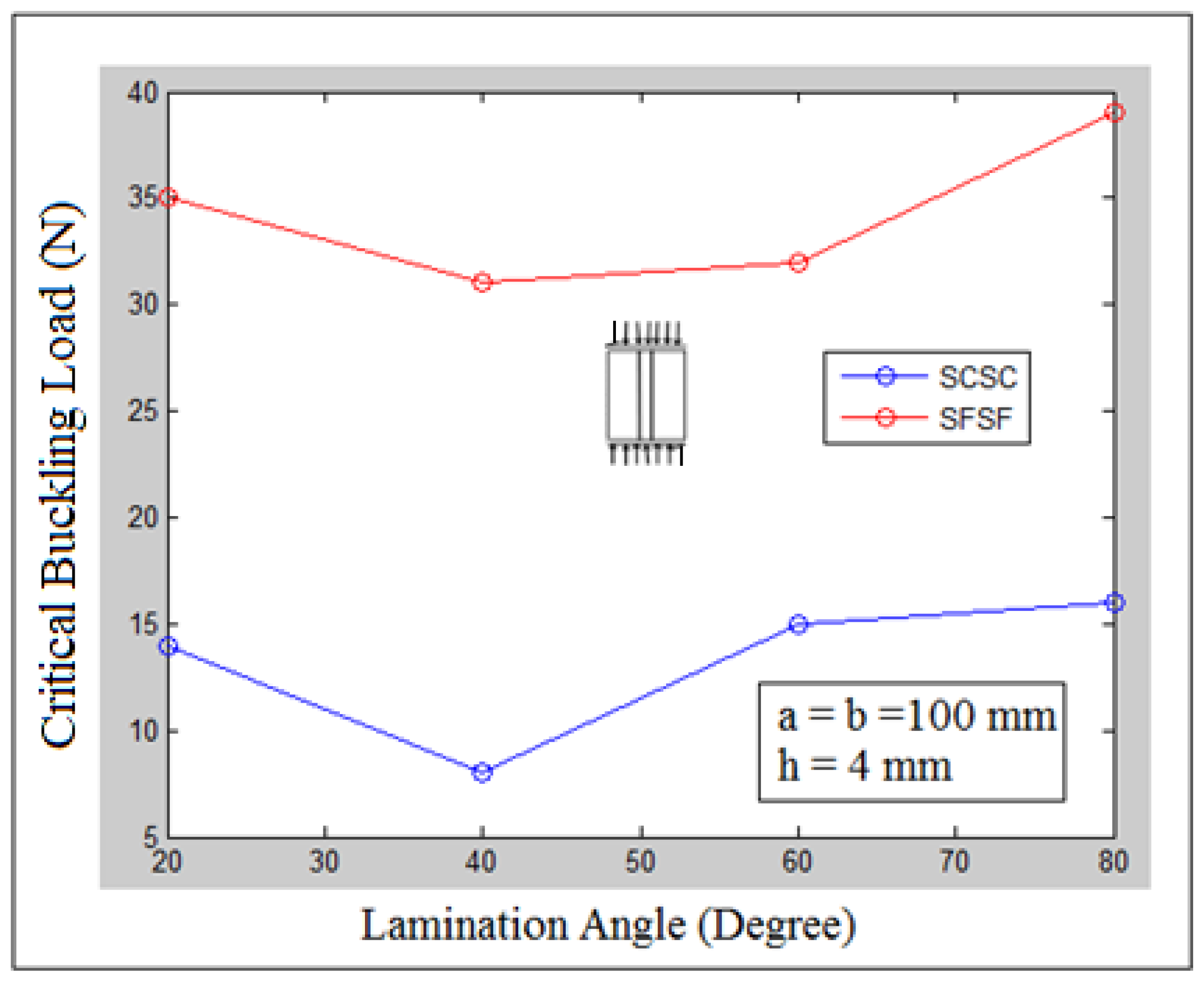
Figure 28 shows the critical buckling load against the lamination angle for the plate with one stiffener for (S-C-S-C and S-F-S-F) different boundary conditions in the presence of the in-plane compression mechanical load and shear force. The critical buckling load is varied sinusoidal for (S-C-S-C) boundary conditions, while the critical buckling load is varied parabolic for (S-F-S-F) boundary conditions. The critical buckling load is the same at the lamination angle (40 and 60) degrees for (S-F-S-F) boundary conditions. The ANSYS program is used in the calculation of the critical buckling load.
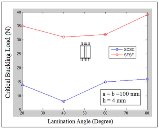
Figure 28.
Critical buckling load against lamination angle for (S-C-S-C) and (S-F-S-F) boundary conditions.
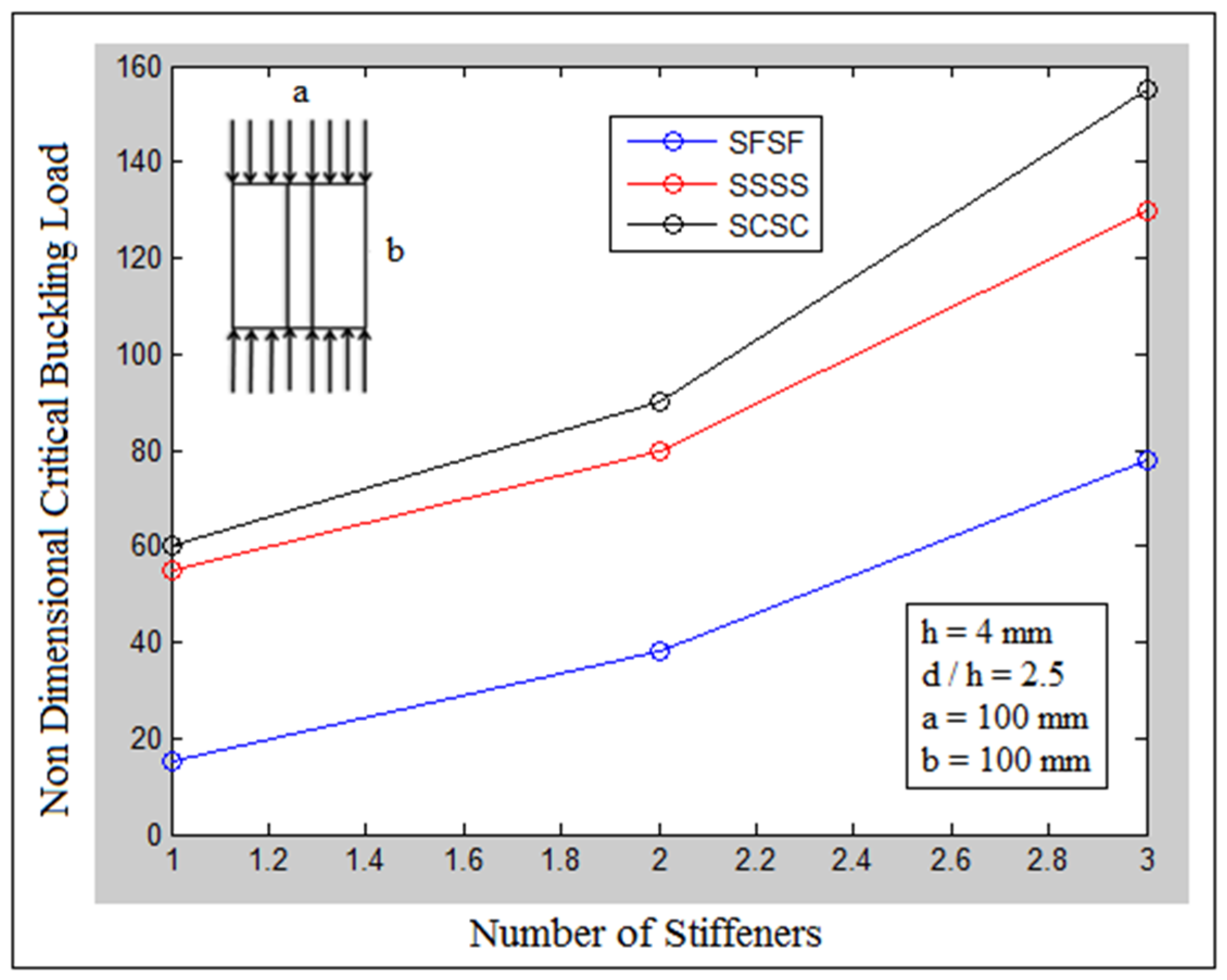
Figure 29 shows the critical buckling load against a number of stiffeners at (S-F-S-F, S-S-S-S and S-C-S-C) boundary conditions in the presence of in-plane compression mechanical load and shear force. The critical buckling load is increased with the increasing of number of stiffeners, while the critical buckling load has a greater value at (S-C-S-C) boundary conditions. The ANSYS program is used in the calculation of the critical buckling load.
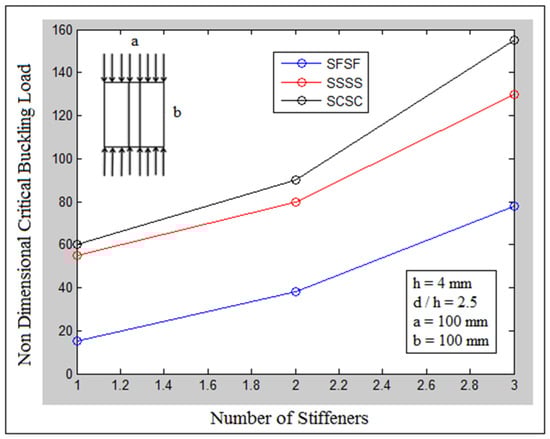
Figure 29.
Critical buckling load against number of stiffeners at (S-F-S-F, S-S-S-S and S-C-S-C) boundary conditions.
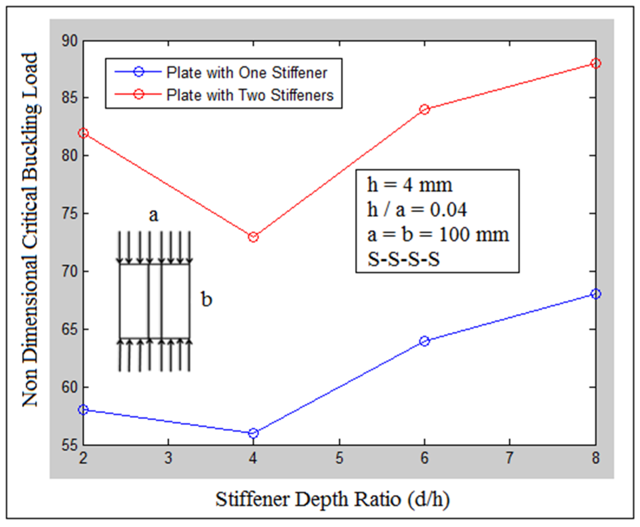
Figure 30 shows the critical buckling load against the stiffener–depth ratio for (S-S-S-S) boundary conditions in the presence of the in-plane compression mechanical load and shear force for the plate with one and two stiffeners. The buckling load is varied sinusoidal with the increasing stiffener–depth ratio. As mentioned, the critical buckling load is increased with the increasing of number of stiffeners. The ANSYS program is used in the calculation of the critical buckling load.
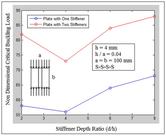
Figure 30.
Critical buckling load against stiffener–depth ratio for (S-S-S-S) boundary conditions.
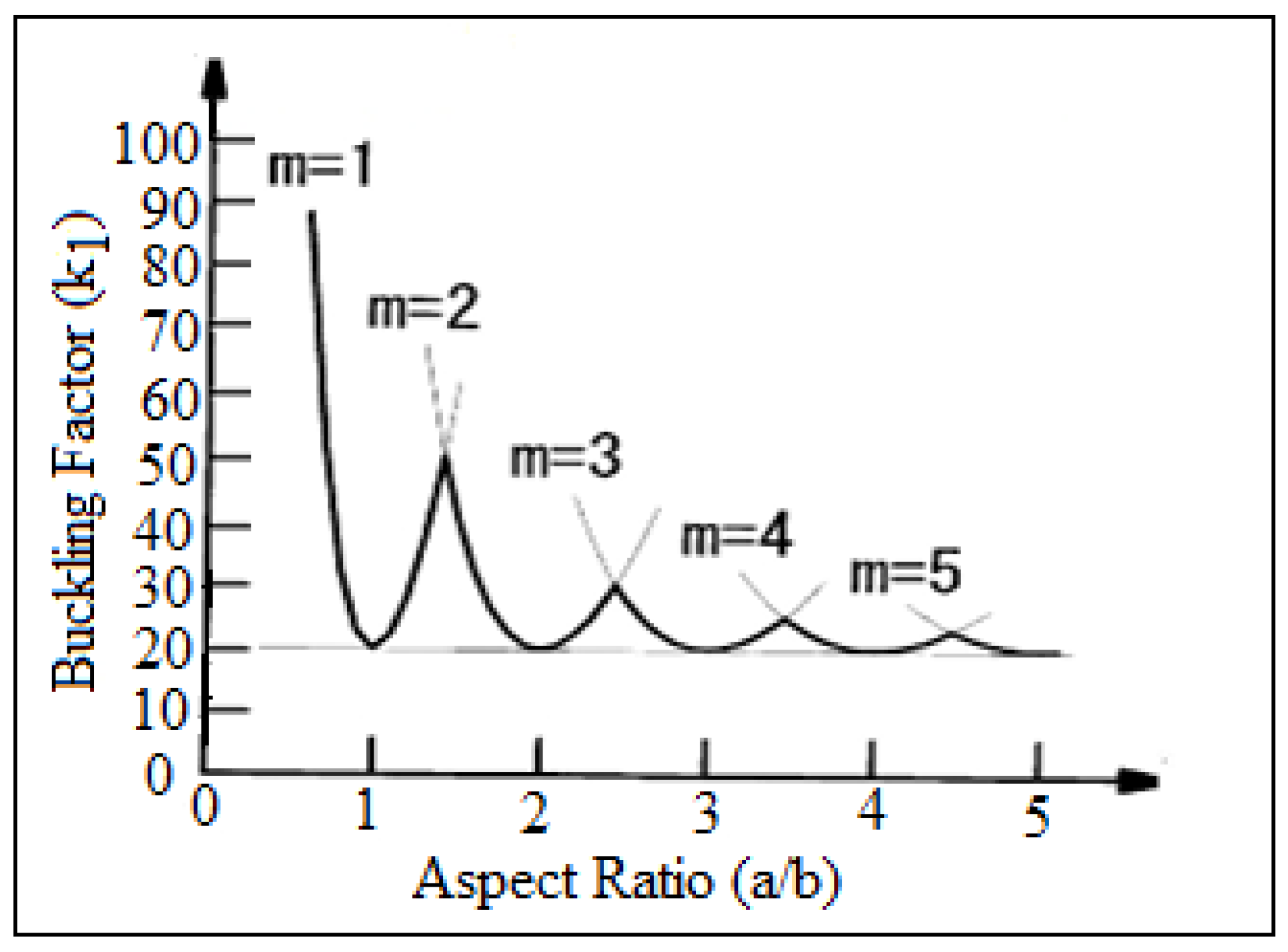
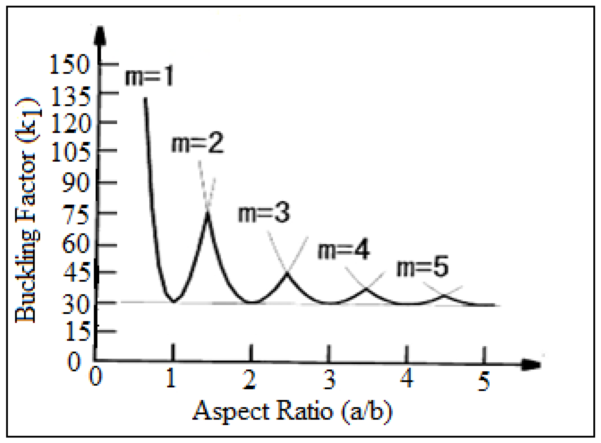
Figure 31 shows the buckling factor against the aspect ratio of (S-S-S-S) boundary conditions for the plate with one stiffener in the presence of in-plane compression mechanical load and shear force. The buckling factor of the buckling mode is decreased with the increasing aspect ratio until it settles down at buckling factor (20). The analytical results of the critical buckling load of the buckling mode have been completed using the Navier solution of classical laminate plate theory. Figure 32 shows the buckling factor against the aspect ratio for the plate with two stiffeners of (S-S-S-S) boundary conditions.
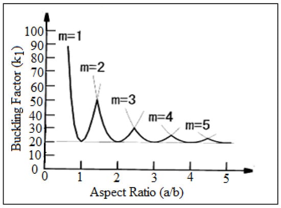
Figure 31.
Buckling factor against aspect ratio for (S-S-S-S) simply supported boundary conditions for plate with one stiffener.
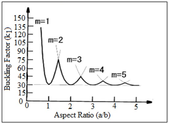
Figure 32.
Buckling factor against aspect ratio for (S-S-S-S) simply supported boundary conditions for plate with two stiffeners.
Table 2 shows the comparison of the critical buckling load when the composite laminated plate is supported with one and two stiffeners at different boundary conditions. The value of the critical buckling load is increased with the increasing of number of stiffeners for different boundary conditions. The numerical results of the critical buckling load were calculated using the ANSYS program, while the analytic results were calculated using the Levy solution of (S-C-S-C, S-C-S-S, S-F-S-C, S-F-S-S and S-F-S-F) boundary conditions. The analytic results of the (S-S-S-S) boundary condition were determined using the Navier solution of classical laminate plate theory.
Table 2.
Comparison critical buckling load at different boundary conditions for one and two stiffeners.
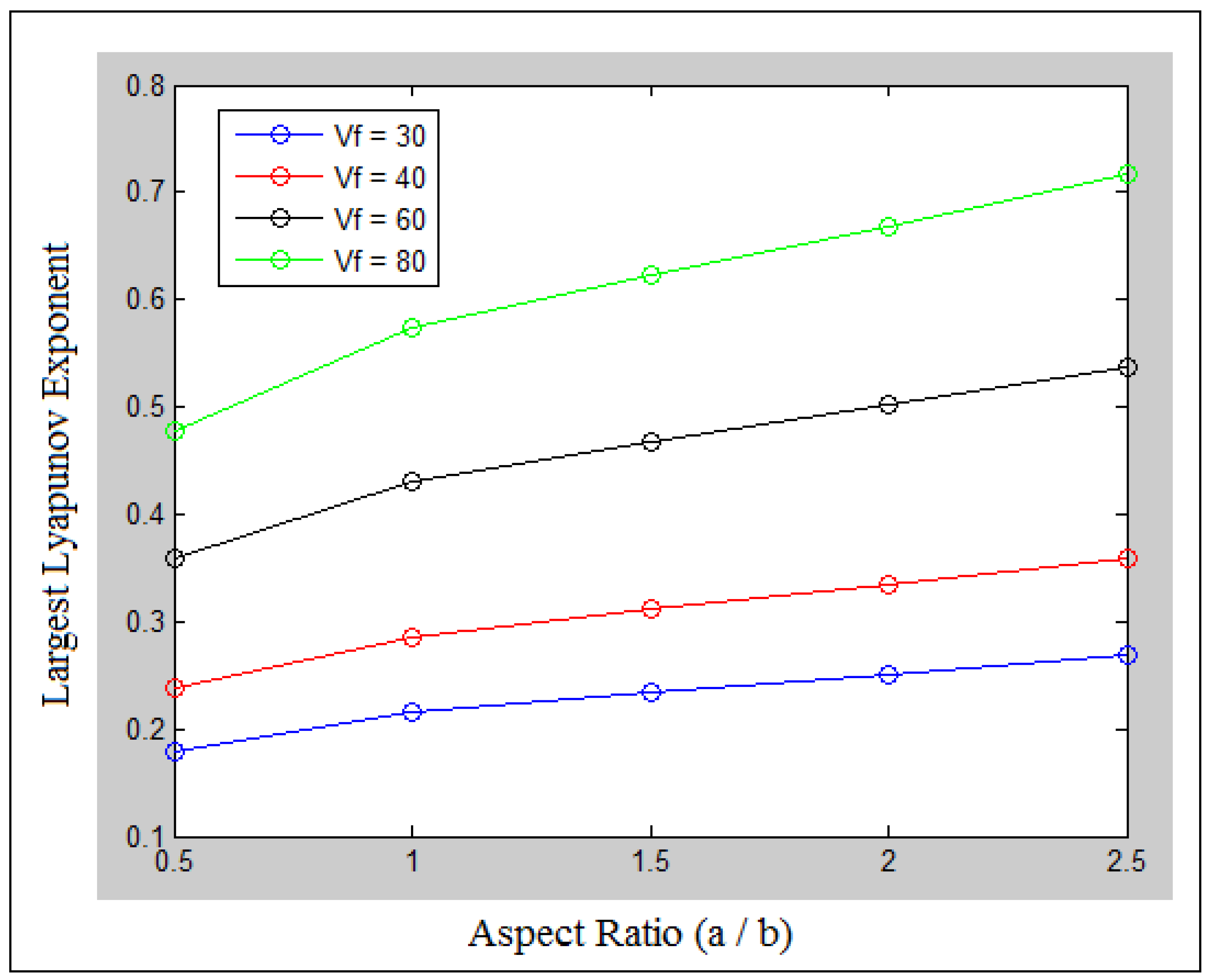
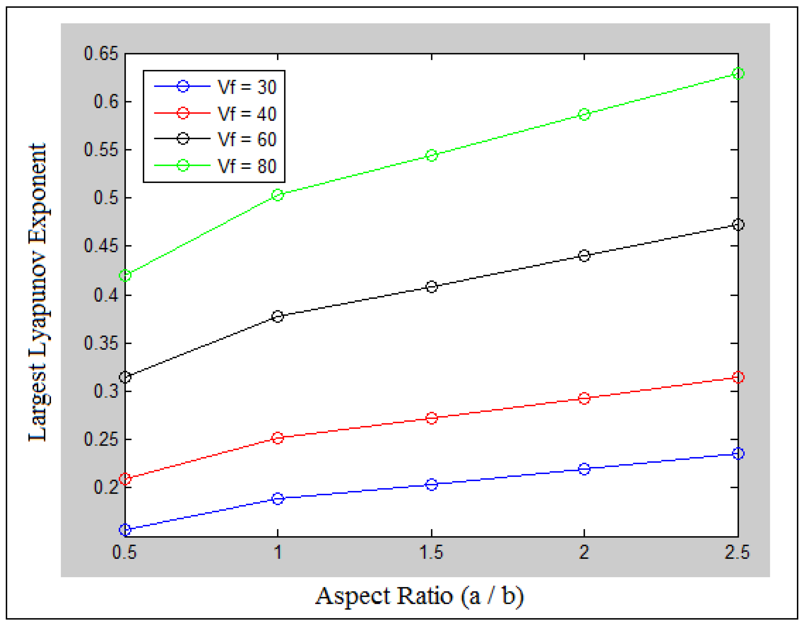
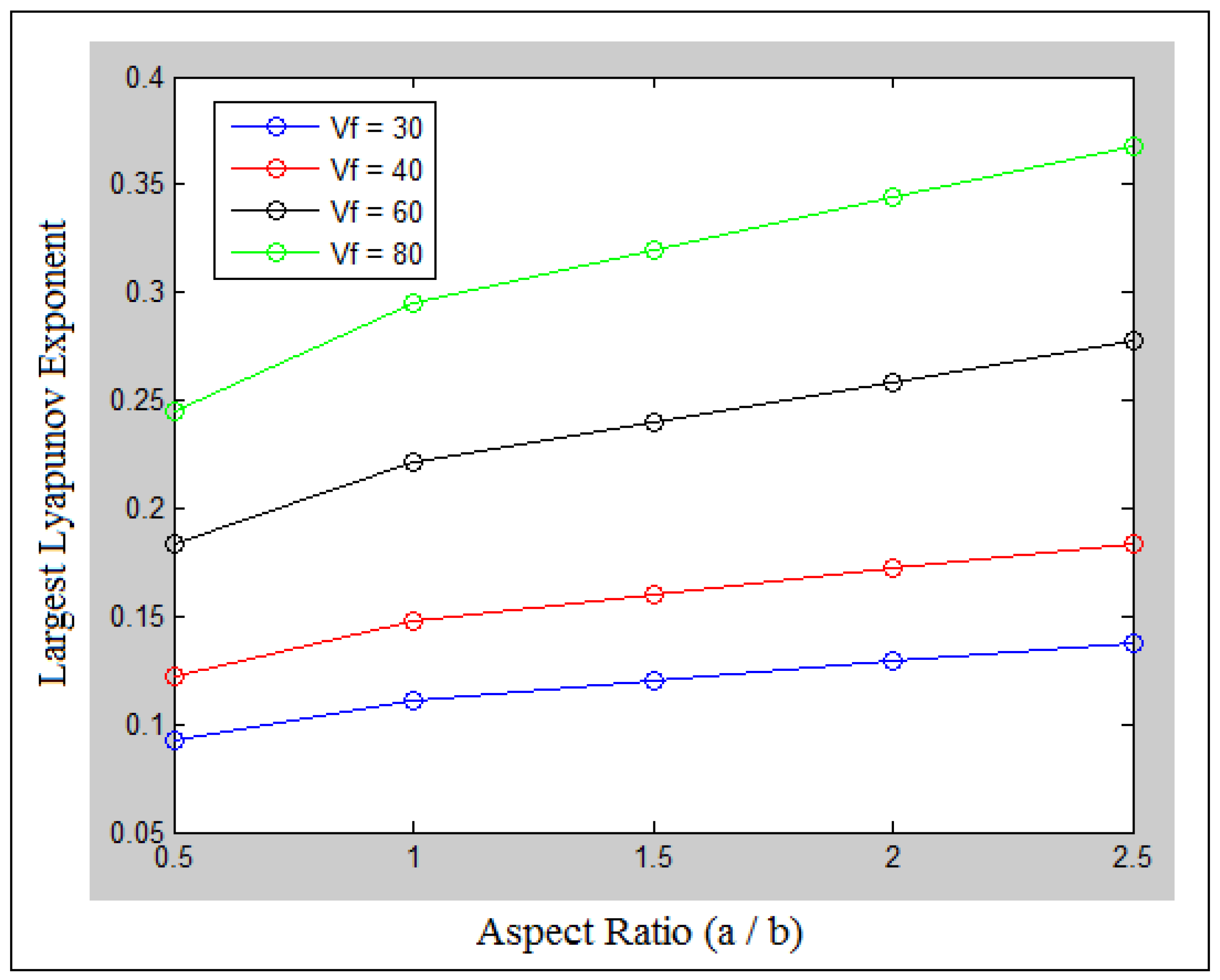
Figure 33, Figure 34 and Figure 35 show the largest Lyapunov exponent against aspect ratios for the un-stiffened plate and plate with one and two stiffeners at different fiber volume fractions. As mentioned, that Lyapunov exponent is the indicator to the non-periodic motion and chaos (nonlinear dynamic phenomena) for the bending deflection of stiffened and un-stiffened composite laminated plate. The nonlinear dynamic behavior of the bending deflection is increased with the increasing of the aspect ratios and fiber volume fractions. All the values of the largest Lyapunov exponent are positive and above zero, which means that the motion of the bending deflection is non-periodic. The nonlinear dynamic phenomena are decreased with the use of beam stiffeners. The system with aspect ratio (2.5) and fiber volume fraction ( = 80%) for the un-stiffened plate is more chaotic than the other systems, as indicated in Figure 33. The nonlinear dynamic phenomena is very low for the system with aspect ratio (2.5) and fiber volume fraction ( = 80%) after using plate with two stiffeners, as shown in Figure 35. The ANSYS program is used in the calculation of bending deflection.
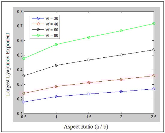
Figure 33.
Largest Lyapunov exponent against aspect ratio for un-stiffened plate at different fiber volume fractions.
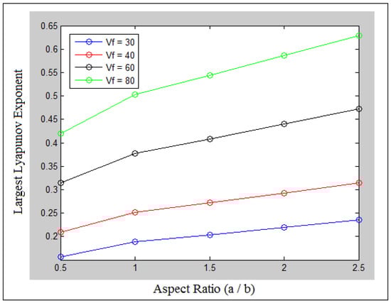
Figure 34.
Largest Lyapunov exponent against aspect ratio for two stiffeners at different fiber volume fractions.
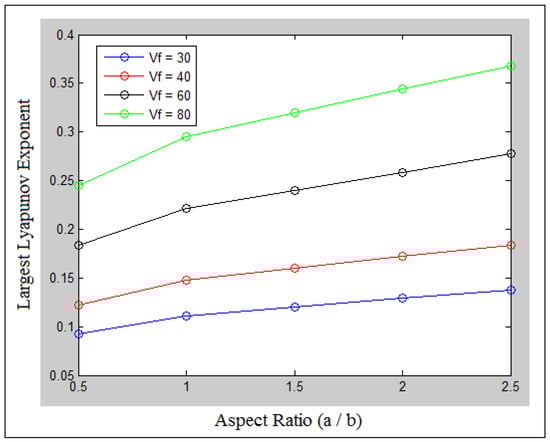
Figure 35.
Largest Lyapunov exponent against aspect ratio for one stiffener at different fiber volume fractions.
Figure 36 and Figure 37 show the comparison of the amplitude of fast Fourier transform (FFT) against frequency at aspect ratio (a/b = 1) and fiber volume fraction ( = 60%) for the plate with two stiffeners. The bending deflection is used in the calculation of the power density function of the fast Fourier transform (FFT). The power of the frequencies’ peaks is disappeared from (FFT) diagram, which gives indication to the chaotic system. The experiment results of the bending deflection were carried out using a strain gauge through a strain meter device, while the numerical results of the bending deflection were completed using the ANSYS program.
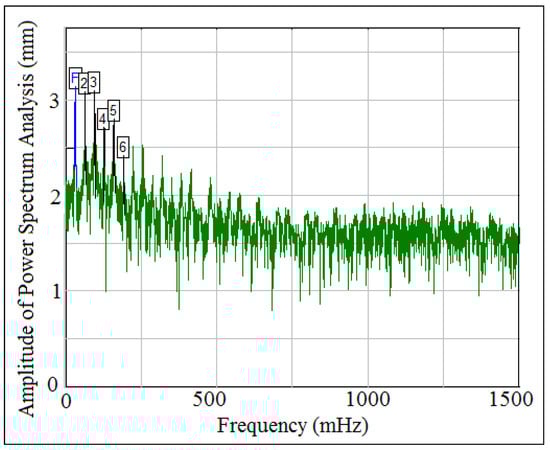
Figure 36.
Power spectrum analysis of experiment test.
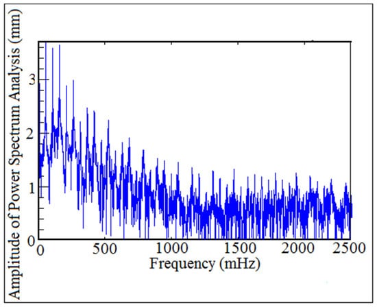
Figure 37.
Power spectrum analysis of numerical simulation.
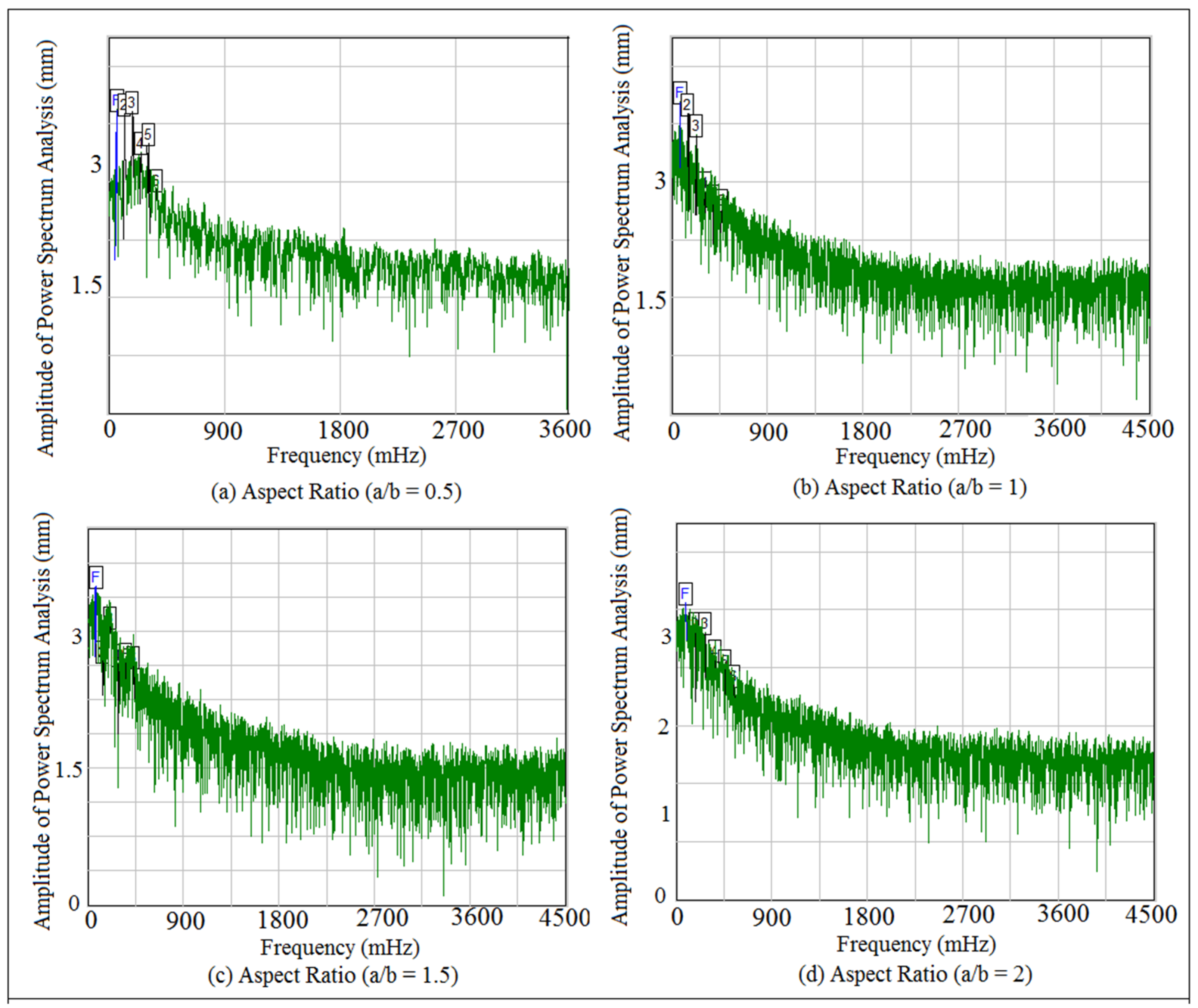
Figure 38 and Figure 39 show the experiment mapping of the amplitude of the fast Fourier transform (FFT) against frequency at different fiber volume fractions and different aspect ratios, respectively. The power density function of the fast Fourier transform (FFT) is decreased with the increasing of fiber volume fractions and aspect ratios. All the systems in Figure 38 and Figure 39 have non-periodic motion, since the frequencies’ peaks start disappearing from the (FFT) diagram for the unstiffened plate and plate with two stiffeners, respectively. The experiment results of the bending deflection were carried out using a strain gauge through a strain meter device.
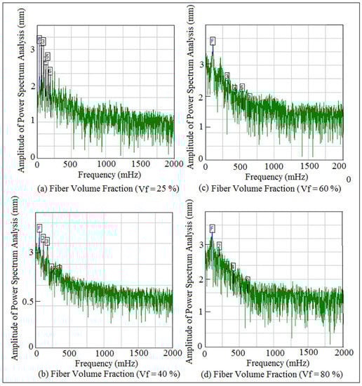
Figure 38.
Mapping of power density function at different fiber volume fractions for un-stiffened plate.
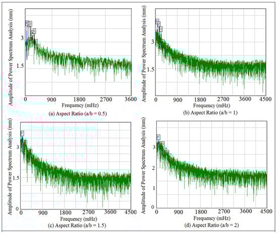
Figure 39.
Mapping of power density function at different aspect ratios for plate with two stiffeners.
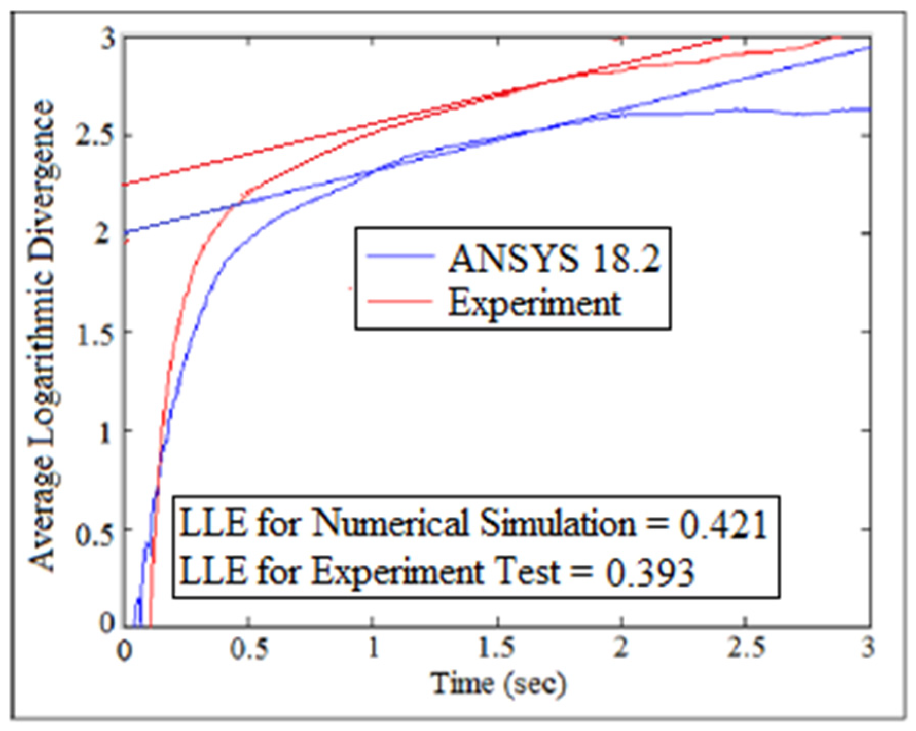
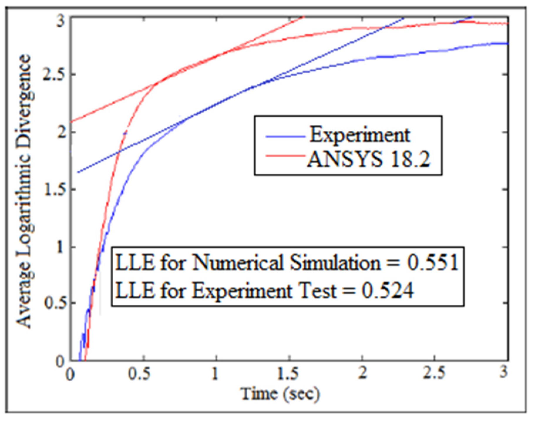
Figure 40 shows the comparison of average logarithmic divergence against time at aspect ratio (a/b = 1.5) and fiber volume fraction ( = 60%). The nonlinear curve represents the average logarithmic divergence of the bending deflection motion for a plate with one stiffener in the presence of an in-plane compression mechanical load and shear force. The straight line represents the slope of average logarithmic divergence, which reflects the value of largest Lyapunov exponent. Moreover, Figure 41 shows the comparison of the average logarithmic divergence against the time at aspect ratio (a/b = 1) and fiber volume fraction ( = 60%) for an un-stiffened plate. The experiment results of the bending deflection that were used in the average logarithmic divergence were carried out using a strain gauge through a strain meter device. The numerical results of the bending deflection were found using the ANSYS program.
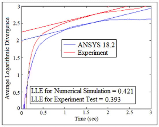
Figure 40.
Comparison of average logarithmic divergence against time for stiffened plate with one stiffener.
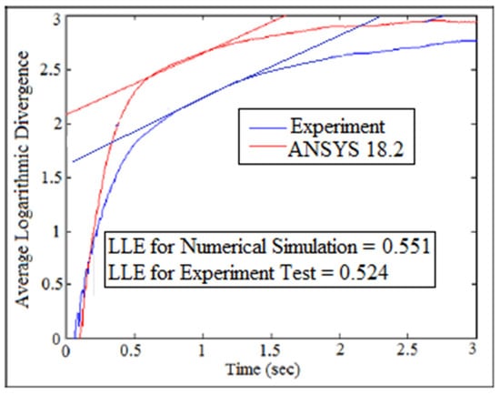
Figure 41.
Comparison of average logarithmic divergence against time for un-stiffened plate.
10. Conclusions
This article discussed how to suppress the nonlinear dynamic phenomena in a composite laminated plate using a beam stiffener in the directions of the applied load. The nonlinear dynamic behavior of the bending deflection was detected using the largest Lyapunov exponent parameter and power density function of the fast Fourier transform (FFT). The nonlinear dynamic behavior of the bending deflection increased with the increase of the aspect ratios and fiber volume fractions. All the values of the largest Lyapunov exponent are positive and above zero, which means that the motion of the bending deflection is non-periodic. The power density function of the fast Fourier transform (FFT) is decreased with the increasing of the fiber volume fractions and aspect ratios. All the systems have non-periodic motion, since the frequencies’ peaks started disappearing from the (FFT) diagram for the unstiffened plate and plate with two stiffeners, respectively. The system with aspect ratio (2.5) and fiber volume fraction ( = 80%) for the un-stiffened plate was more chaotic than the other systems. The nonlinear dynamic phenomena was very low for the system with aspect ratio (2.5) and fiber volume fraction ( = 80%) after using the plate with two stiffeners.
Funding
This research received no external funding.
Data Availability Statement
The author declares that the manuscript data will be available to the public upon request.
Acknowledgments
I want to first thank the reviewers and the editor for reviewing my paper. Additionally, I want to acknowledge the Department of Mechanical Engineering at the University of Baghdad for their total support for finishing this research.
Conflicts of Interest
The author declares that he has no conflict of interest.
Nomenclature
| a | Length of large span of rectangular plate, mm |
| b | Length of small span of rectangular plate, mm |
| h | Thickness of the composite plate, mm |
| , | Lamina stresses field vector, N/mm2 |
| , | Extensional strain vector |
| , | Flexural (bending) strain vector |
| , | Displacement components in the 2-D coordinate system, mm |
| Reduced stiffness elements, N/mm2 | |
| Mid plane deflection along z-direction, mm | |
| Volume fraction for the fiber | |
| Fiber weight fraction | |
| Mass density for the fiber, kg | |
| Mass density for the composite, kg | |
| , | Modulus of elasticity along (x and y) directions, respectively, N/mm2 |
| , | Poisson’s ratio in plane 1-2 and the perpendicular plane 2-1, respectively |
| Thickness, depth, distance between stiffeners when the stiffener placed along x-axis, mm | |
| Thickness, depth, distance between stiffeners when the stiffener placed along y-axis, mm | |
| Critical buckling load, N | |
| Mass per unit area of the composite plate, kg/m2 | |
| m, n | Double trigonometric of Fourier series |
| Natural frequency of the composite laminated plate | |
| Buckling factor | |
| GFNN | Global false nearest neighbors for extracting embedding dimensions |
| AMI | Average mutual information algorithm for quantifying time delay |
| D | Distance between trajectories |
| d(t) | Percentage of variation in the distance between trajectories |
| Distance between the pair (j-th) at nearest neighbors (i) of the trajectories | |
| t | Time strides |
| y(i) | Data of follower displacement after curve fitting |
| Δt | Various time strides |
| λ | Largest Lyapunov exponent parameter |
| S-S-S-S | Simply-simply-simply-simply supported boundary conditions |
| S-F-S-F | Simply-free-simply-free supported boundary conditions |
| S-C-S-C | Simply-clamped-simply-clamped supported boundary conditions |
| S-F-S-S | Simply-free-simply-simply supported boundary conditions |
| S-F-S-C | Simply-free-simply-clamped supported boundary conditions |
| S-C-S-S | Simply-clamped-simply-simply supported boundary conditions |
Appendix A
B.C. (1) At y = 0, ,
B.C. (2) At y = b, ,
The expressions (, , , ) can be prepared before I substitute for the boundary conditions:
Apply the boundary conditions listed above on Equation (9) and after simplification to obtain
After simplification, Equations (A1)–(A4) will be
where
And;
A, B, C, D, E, F, G, H, I, J, K, L and M are constants.
Maple software is used to solve for the constants , , ):
Substitute the constants , , ) into Equation (9) to obtain the general equation of the plate. Solve for the plate equation to determine the in-plane compression mechanical load and derive the output equation with respect to the buckling mode (m) along the x-axis to calculate the critical buckling load. From Equation (A1), the critical buckling load can be calculated as below in the following equation:
where
Derive Equation (A13) with respect to ():
Solve Equation (A14) to find the buckling mode:
Substitute Equation (A15) into Equation (A13) to determine the critical buckling load:
Appendix B
The constants (A, B, C, D, E, F, G, H, I, J, K, L and M) and , , ) using different boundary conditions are as below:
- (1)
- (S-C-S-C) Boundary Conditions:
- (2)
- (S-C-S-S) Boundary Conditions:
- (3)
- (S-F-S-C) Boundary Conditions:
- (4)
- (S-F-S-S) Boundary Conditions:
References
- Keshav, V.; Patel, S.N. Non-Linear dynamic pulse buckling of laminated composite curved panels. J. Struct. Eng. Mech. 2020, 73, 181–190. [Google Scholar]
- Mondal, S.; Ramachandra, L.S. Nonlinear Dynamic Pulse Buckling of Imperfect Laminated Composite Plate with Delamination. Int. J. Solids Struct. 2020, 198, 170–182. [Google Scholar]
- Taczała, M.; Buczkowski, R.; Kleiber, M. Nonlinear buckling and post-buckling response of stiffened FGM plates in thermal environments. J. Compos. Part B Eng. 2017, 109, 238–247. [Google Scholar]
- Tao, Z.; Tu-guang, L.; Yao, Z.; Luo, J. Nonlinear dynamic buckling of stiffened plates under in-plane impact load. J. Zhejiang Univ. Sci. A 2004, 5, 609–617. [Google Scholar]
- Yousuf, L.S. Nonlinear dynamics investigation of flexural stiffness of composite laminated plate under the effect of temperature and combined loading using Lyapunov exponent parameter. J. Compos. Part B Eng. 2021, 219, 108926. [Google Scholar] [CrossRef]
- Yousuf, L.S. Nonlinear dynamics simulation of bending deflection for composite laminated plate under varied temperature using Lyapunov exponent parameter. In Proceedings of the ASME 2021 International Design Engineering Technical Conferences and Computers and Information in Engineering Conference 2021, Online, 17–19 August 2021. [Google Scholar]
- Hegaze, M.H. Nonlinear Dynamic Analysis of Stiffened and Unstiffened Laminated Composite Plates Using a High-order Element. J. Compos. Mater. 2009, 44, 327–346. [Google Scholar] [CrossRef]
- Less, H.; Abramovich, H. Dynamic buckling of a laminated composite stringer–stiffened cylindrical panel. J. Compos. Part B Eng. 2012, 43, 2348–2358. [Google Scholar] [CrossRef]
- Aboudi, J.; Gilat, R. The Lyapunov exponents as a quantitative criterion for the dynamic buckling of composite plates. Int. J. Solids Struct. 2002, 39, 467–481. [Google Scholar]
- Chai, Y.Y.; Li, F.M.; Song, Z.G. Nonlinear Vibration Behaviors of Composite Laminated Plates with Time-Dependent Base Excitation and Boundary Conditions. Int. J. Nonlinear Sci. Numer. Simul. 2017, 18, 145–161. [Google Scholar] [CrossRef]
- Borkowski, L. Numerical analysis of dynamic stability of an isotropic plate by applying tools used in dynamics. Dyn. Syst. Theory Appl. 2017, 248, 63–73. [Google Scholar]
- Kim, H.G. Experimental nonlinear dynamics and snap-through of post-buckled composite plates. Nonlinear Dyn. 2017, 1, 21–35. [Google Scholar]
- Pan, N. Theoretical determination of the optimal fiber volume fraction and fiber-matrix property compatibility of short fiber composites. Polym. Compos. 1993, 14, 85–93. [Google Scholar] [CrossRef] [Green Version]
- Gopalan, V.; Suthenthiraveerappa, V.; David, J.S.; Subramanian, J.; Annamalai, A.R.; Jen, C.P. Experimental and Numerical Analyses on the Buckling Characteristics of Woven Flax/Epoxy Laminated Composite Plate under Axial Compression. Polymers 2021, 13, 995. [Google Scholar] [CrossRef] [PubMed]
- Sun, C.T. Mechanics of Aircraft Structures, 2nd ed.; Wiley: Hoboken, NJ, USA, 2021. [Google Scholar]
- Thompsom, M.K.; Thompson, J.M. ANSYS Mechanical APDL for Finite Element Analysis; Butterworth-Heinemann: Oxford, UK, 2017. [Google Scholar]
- Parlitz, U. Estimating lyapunov exponents from time series. In Chaos Detection and Predictability; Springer: Berlin/Heidelberg, Germany, 2016; Volume 915, pp. 1–34. [Google Scholar]
- Terrier, P.; Fabienne, R. Maximum Lyapunov exponent revisited: Long-term attractor divergence of gait dynamics is highly sensitive to the noise structure of stride intervals. Gait Posture 2018, 66, 236–241. [Google Scholar] [CrossRef] [PubMed] [Green Version]
- Hussain, V.S.; Spano, M.L.; Lockhart, T.E. Effect of data length on time delay and embedding dimension for calculating the Lyapunov exponent in walking. J. R. Soc. Interface 2020, 17, 20200311. [Google Scholar] [CrossRef] [PubMed]
- Garcia, M.M.; Morales, I.; Rodriguez, J.M.; Marin, M.R. Selection of embedding dimension and delay time in phase space reconstruction via symbolic dynamics. Entropy 2021, 23, 221. [Google Scholar] [CrossRef] [PubMed]
- Stoica, P.; Moses, R.L. Spectral analysis of signals. In Digital Signal Processing; Rao, K.D., Swamy, M.N.S., Eds.; Springer: Berlin/Heidelberg, Germany, 2005; pp. 721–751. [Google Scholar]


Publisher’s Note: MDPI stays neutral with regard to jurisdictional claims in published maps and institutional affiliations. |
© 2022 by the author. Licensee MDPI, Basel, Switzerland. This article is an open access article distributed under the terms and conditions of the Creative Commons Attribution (CC BY) license (https://creativecommons.org/licenses/by/4.0/).