Abstract
In recent years, Convolutional Neural Network (CNN) has become an attractive method to recognize and localize plant species in unstructured agricultural environments. However, developed systems suffer from unoptimized combinations of the CNN model, computer hardware, camera configuration, and travel velocity to prevent missed detections. Missed detection occurs if the camera does not capture a plant due to slow inferencing speed or fast travel velocity. Furthermore, modularity was less focused on Machine Vision System (MVS) development. However, having a modular MVS can reduce the effort in development as it will allow scalability and reusability. This study proposes the derived parameter, called overlapping rate (), or the ratio of the camera field of view () and inferencing speed () to the travel velocity () to theoretically predict the plant detection rate () of an MVS and aid in developing a CNN-based vision module. Using performance from existing MVS, the values of at different combinations of inferencing speeds (2.4 to 22 fps) and travel velocity (0.1 to 2.5 m/s) at 0.5 m field of view were calculated. The results showed that missed detections occurred when was less than 1. Comparing the theoretical detection rate () to the simulated detection rate () showed that had a 20% margin of error in predicting plant detection rate at very low travel distances (<1 m), but there was no margin of error when travel distance was sufficient to complete a detection pattern cycle (≥10 m). The simulation results also showed that increasing or having multiple vision modules reduced missed detection by increasing the allowable . This number of needed vision modules was equal to rounding up the inverse of . Finally, a vision module that utilized SSD MobileNetV1 with an average effective inferencing speed of 16 fps was simulated, developed, and tested. Results showed that the and had no margin of error in predicting of the vision module at the tested travel velocities (0.1 to 0.3 m/s). Thus, the results of this study showed that can be used to predict and optimize the design of a CNN-based vision-equipped robot for plant detections in agricultural field operations with no margin of error at sufficient travel distance.
1. Introduction
The increasing cost and decreasing availability of agricultural labor [1,2] and the need for sustainable farming methods [3,4,5] led to the development of robots for agricultural field operations. However, despite the success of robots in industrial applications, agricultural robots for field operations remain primarily in the development stage due to the complex characteristics of the farming environment, high cost of development, and high durability, functionality, and reliability requirements [6,7,8].
As a potential solution to these challenges, field robots with computer vision have been increasing due to the large amount of information that can be extracted from an agricultural scene [9]. Real-time machine vision systems (MVS) are often used to recognize, classify and localize plants accurately for precision spraying [10,11], mechanical weeding [12], solid fertilizer application [13], and harvesting [14,15]. However, using traditional image processing techniques, early machine vision implementations for field operations were difficult due to the vast number of features needed to model and differentiate plant species [13] and work at various farm scenarios [12].
Recently, developments in deep learning allowed Convolutional Neural Networks (CNN) to be used for accurate plant species detection and segmentation [16,17]. However, despite high classification and detection performance, the large computational power requirement of CNN limits its application in real-time operations [18]. As a result, most CNN applications in agriculture were primarily employed in non-real-time scenarios, excluding inferencing speeds in the evaluated parameters among related studies. For example, a study that surveyed CNN-based weed detection and plant species classification reported 86–97% and 48–99% precisions, respectively, but data on inferencing speeds were unreported [19]. Similarly, research on fruit classification and recognition using CNN showed 77–99% precision, but inferencing speeds were also excluded in the measured parameters [19,20,21].
Few studies have evaluated the real-time performance of CNNs for agricultural applications. For example, in a study by Olsen et al. (2019) [22] on detecting different species of weeds, the real-time performance of ResNet-50 in an NVIDIA Jetson TX2 was only 5.5 fps at 95.1% precision. Optimizing their TensorFlow model using TensorRT increased the inferencing speed to 18.7 fps. The study of Chechliński et al. (2019) [23] using a custom CNN architecture based on U-Net, MobileNets, DenseNet, and ResNet in a Raspberry Pi 3B+ resulted in only 60.2% precision at 10.0 fps. Finally, Partel et al. (2019) [11] developed a mobile robotic sprayer that used YOLOv3 running on an NVIDIA 1070TI at 22 fps and NVIDIA Jetson TX2 at 2.4 fps for real-time crop and weed detection and spraying. The vision system with 1070TI had 85% precision, while the TX2 vision system had 77% precision. Furthermore, the system with TX2 missed 43% of the plants because of its slow inferencing speed. Conversely, the CNN-based sprayer with the faster 1070TI, resulting in higher inferencing speed, only missed 8% of the plants.
However, the travel velocities of surveyed systems were often unevaluated despite operating in real-time. Additionally, theoretical approaches to quantify and account for the effect of travel velocity on the capability of the vision system to sufficiently capture discrete data and effectively represent a continuous field scenario were often not included in the design. Other studies, on the contrary, evaluated the effect of travel velocity on CNN detection performance, but the impact of inferencing speed remained unevaluated. For instance, in the study of Liu et al. (2021) [24], the deep learning-based variable rate agrochemical spraying system for targeted weeds control in strawberry crops equipped with a 1080TI showed increasing missed detections, as travel velocity increases regardless of CNN architecture (VGG-16, GoogleNet or AlexNet). At 1, 3, and 5 km/h, their system missed 5–9%, 6–10%, and 13–17% of the targeted weeds, respectively.
The brief review of the developed systems showed that inferencing speed () and travel velocity () of a CNN-based MVS impact its detection rate (). is the fraction of the number of detected plants to the total number of plants and was often expressed as the recall of the CNN model [11,24,25]. However, a theoretical approach to predict the of a CNN-based MVS as affected by both and is yet to be explored.
Current approaches in developing a mechatronic system with CNN-based MVS involve building and testing an actual system to determine [11,24,25]. However, building and testing several CNN-based MVS to determine the effect of and on would be very tedious as the process would involve building the MVS hardware, image dataset preparation, training multiple CNN models, developing multiple software frameworks to integrate the different CNN models into the vision system, and testing the MVS. Hence, this study also proposes to use computer simulation, in addition to theoretical modeling, in predicting as a function of the mentioned parameters, to reduce the difficulty of selecting and sizing the components of the CNN-based MVS.
Computer simulations were often used to characterize the effect of design and operating parameters on the overall performance of agricultural robots for field operations. For example, Villette et al. (2021) [26] demonstrated that computer simulations could be used to estimate the required sprayer spatial resolution of vision-equipped boom sprayer, as affected by boom section weeds, nozzle spray patterns, and spatial weed distribution. Wang et al. (2018) [27] used computer modeling and simulation to identify potential problems of a robotic apple picking arm and developed an algorithm to improve the performance by 81%. Finally, Lehnert et al. (2019) [28] used modeling and computer simulation to create a novel multi-perspective visual servoing technique to detect the location of occluded peppers. However, the use of simulation to quantify the effects of , , and camera configurations on of an MVS remain unexplored.
Furthermore, a survey of review articles showed that almost all robotic systems in agriculture employ fixed configurations and are non-scalable, resulting in less adaptability to complex agricultural environments [7,8,29,30]. Thus, aside from modeling and simulation, this study also proposes a module-based design approach to enable reusability and scalability by minimizing production costs and shortening the lead time of machine development [31]. A module can be defined as a repeatable and reusable machine component that performs partial or full functions and interact with other machine components, resulting in a new machine with new overall functionalities [32].
Therefore, this study proposes theoretical and simulation approaches in predicting combinations of , , and camera configuration to prevent missed plant detections and aid in developing a modular CNN-based MVS. In particular, based on the brief literature review and identified research gaps, the study specifically aims to make the following contributions:
- The introduction of a dimensionless parameter, called overlapping rate (), which is a quantitative predictor of as a function of and , for a specific camera field of view ();
- A set of Python scripts containing equations and algorithms to model a virtual field, simulate the motion of the virtual camera, and perform plant hill detection;
- An evaluation of based on different combinations of published and from existing systems through the proposed theoretical approach and simulation;
- A detailed analysis through simulation of the concept of increasing or using several adjacent synchronous cameras () to prevent missed detections in MVS with low at high ; and
- A reusable and scalable CNN-based vision module for plant detection based on Robot Operating System (ROS) and the Jetson Nano platform.
2. Materials and Methods
2.1. Concept
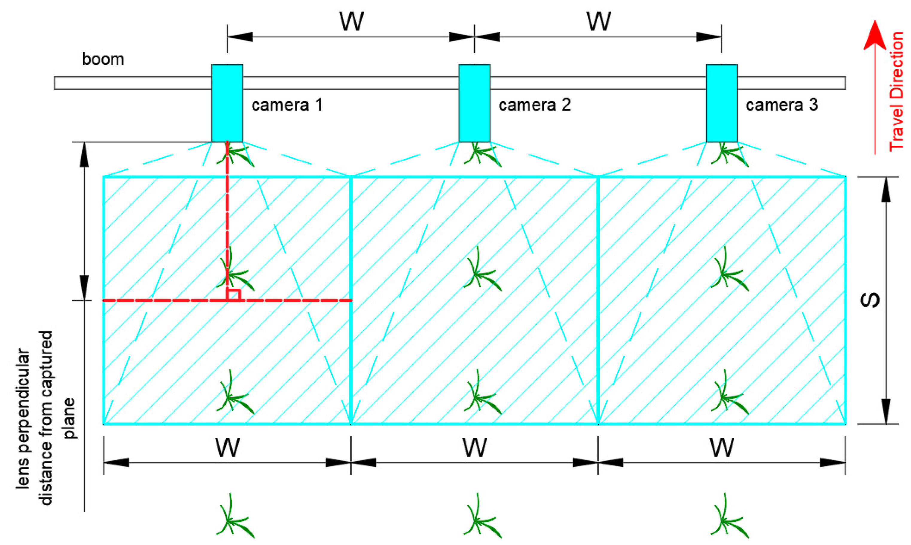
Cameras for plant detection are typically mounted on a boom of a sprayer or fertilizer spreader [10,11,13], as illustrated in Figure 1. They are oriented so that their optical axis is perpendicular to the field and captures top-view images of plants [33].
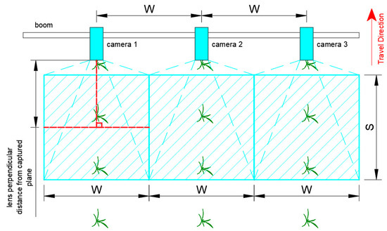
Figure 1.
Camera mounting location and orientation in a boom (not drawn in scale).
Depending on the distance between the camera lens and captured plane, lens properties, and sensor size, the frame width or height is equivalent to an actual linear distance. For simplicity, the linear length of the side of a field of view of a frame parallel to the direction of travel shall be denoted as , in meters per frame. To provide complete visual coverage of the traversed width of the boom, the maximum spacing between adjacent cameras is equal to the length of the side of a field of view of a frame perpendicular to the direction of travel, denoted as , in meters per frame [10].
During motion, the traverse distance between two consecutive frames of the camera (, in meters, is equal to the product of travel velocity (), in m/s, and the time between the frames (), in seconds, as illustrated in Equation (1).
The ratio of to is proposed as the overlapping rate (), a dimensionless parameter, and is represented by Equation (2).
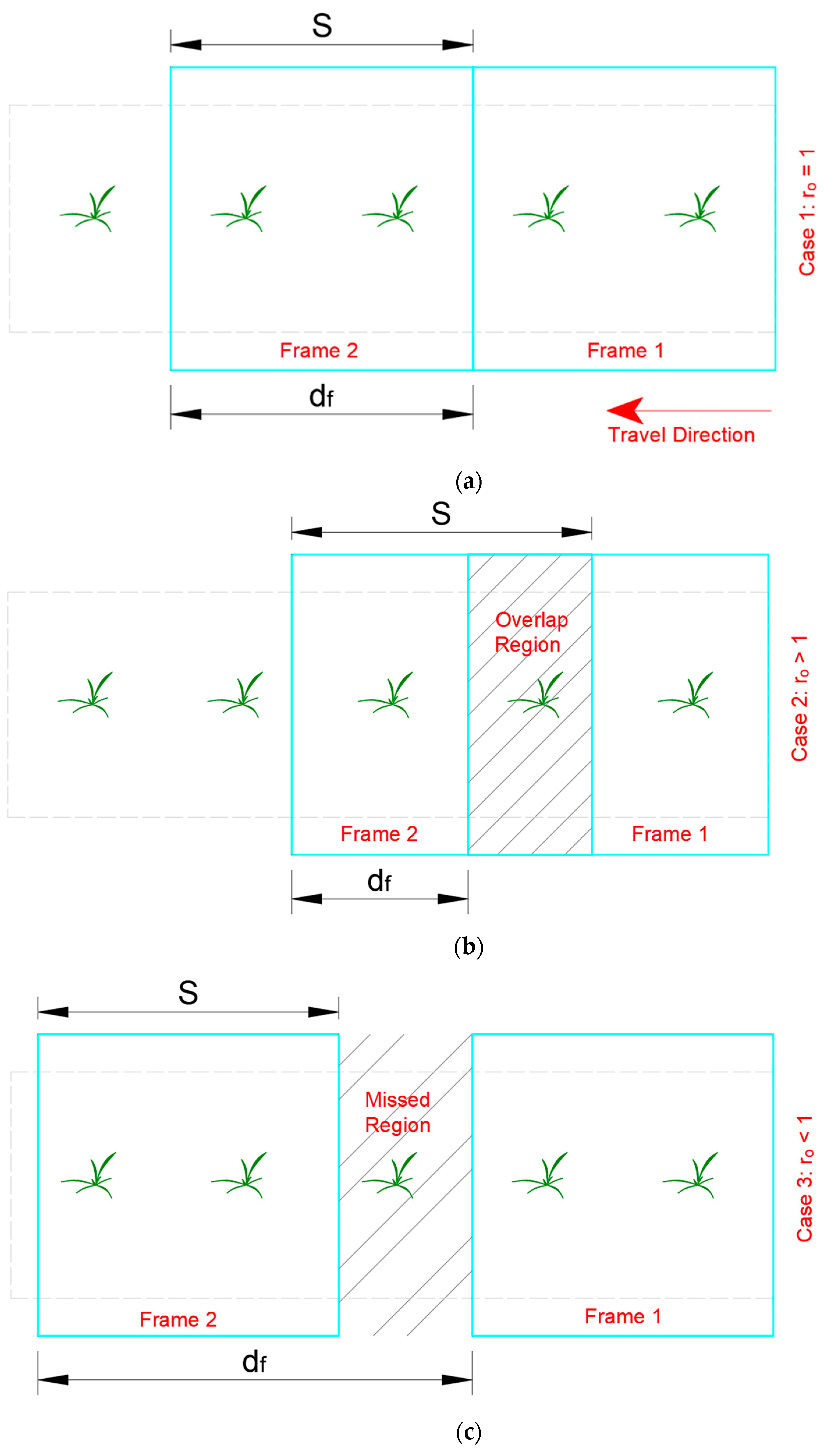
With a single camera, the value of describes whether there is an overlap or gap between frames. Depending on the value of , certain regions in the traversed field of the machine, with a single camera configuration, will be uniquely captured, captured in multiple frames, or completely missed, as shown in Figure 2 and illustrated by the following cases:
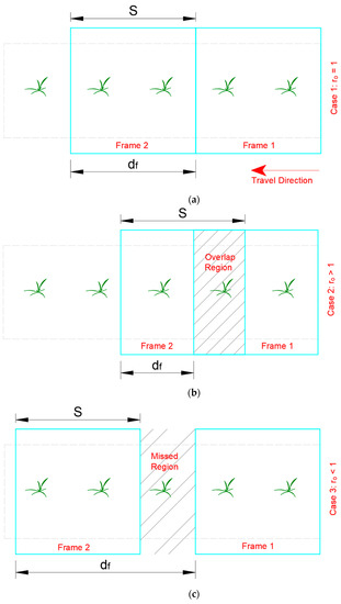
Figure 2.
Relative positions of two consecutive processed frames of a vision system: (a) since = , resulting in frames with unique bounded regions; (b) since < , resulting in overlap region (b); and (c) since > , resulting in missed region.
- Case 1: ro = 1. When and are equal, the extents of each consecutive processed frame are side by side. Hence, both gaps and overlaps are absent. This scenario is ideal since the vehicle velocity and camera frame rate match perfectly.
- Case 2: . The vision system accounted for all regions in the traversed field, but there is an overlap between the frames. The length of the current frame that is already accounted for by the previous one is . The vehicle can run faster if the mechanical capacity allows.
- Case 3: . Gaps will occur between each pair of consecutive frames, and the camera will miss certain plants. The length of each gap is . We can define a gap rate () as shown in Equation (3) to depict the significance of the gap.
2.1.1. Theoretical Detection Rate
The theoretical or maximum detection rate () can be defined as , shown in Equation (4). The was also a dimensionless parameter.
2.1.2. Maximizing Travel Velocity
Setting in Equation (2) resulted in Equation (5), which is similar to the equation used by Esau et al. (2018) [10] in calculating the maximum travel velocity of a sprayer. However, Equation (5) only describes the maximum forward velocity that a vision-equipped robot can operate to prevent gaps while traversing the field as a function of and .
2.1.3. Increasing
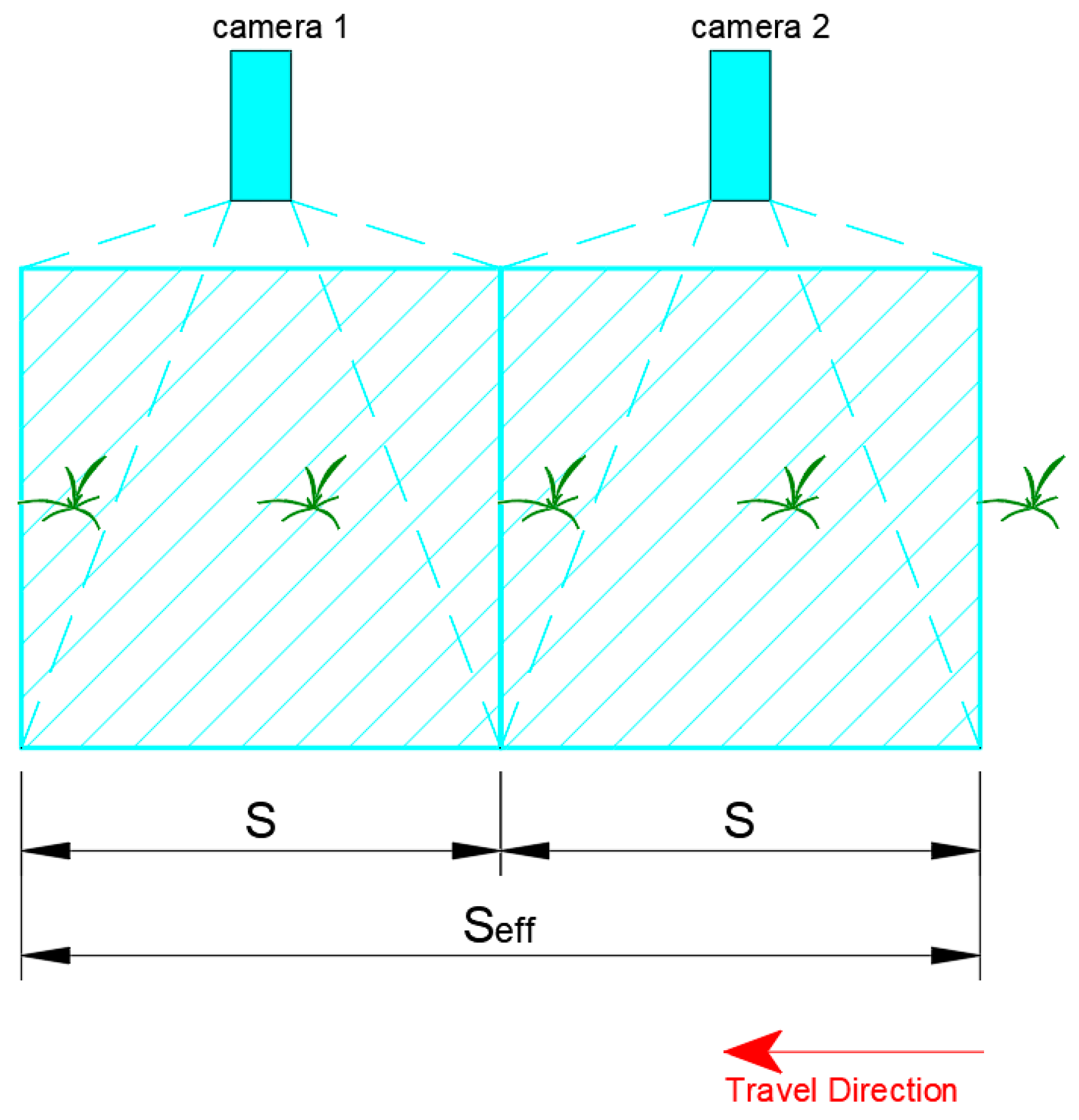
A consequence of Equation (5) was that increasing the length of the frame at a constant shall increase . Hence, raising the camera mounting height or using multiple adjacent synchronous cameras along a single plant row can increase the effective . This situation, then, shall increase without the need for powerful hardware for a faster inferencing speed. When , the number of vision modules () to prevent missed detection can be calculated using Equation (6). Since represents the fraction of the field that can be covered by a single camera, the inverse of represents the number of adjacent cameras that will result in 100% field coverage. The calculated inverse was rounded up to the following number, as cameras are discrete elements.
The effective actual ground distance (, in meters, captured side-by-side by identical and synchronous vision modules without gaps and overlaps is equal to the product of and , as shown in Equation (7). This configuration will then allow the use of less powerful devices while operating at the required of an agricultural field operation such as spraying, as illustrated in Figure 3.
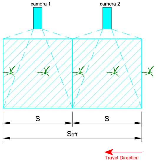
Figure 3.
Multiple adjacent cameras for plant detection at . Thus, .
2.2. Field Map Modeling
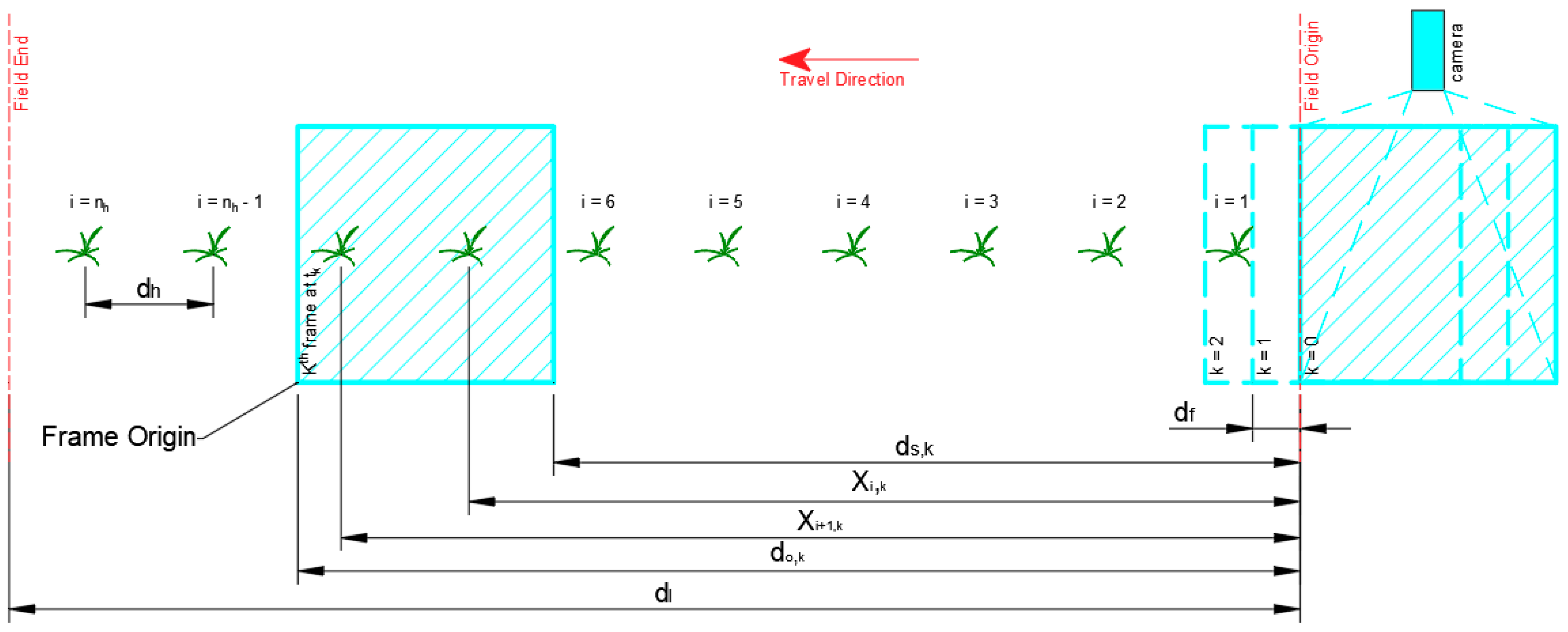
A virtual field was prepared to test the concepts that were presented. A 1000 m field length () with crops planted in hills at 0.2 m hill spacings () was used. The number of hills () and plant hill locations (), in meters, in the entire field length were calculated using Equations (8) and (9), respectively. A section of the virtual field is presented in Figure 4.

Figure 4.
Virtual field with field map and motion modeling parameters. The frame at k = 0 represents the frame just outside the virtual field. The frame at k = 1 represents the first frame that entered the virtual field.
2.3. Motion Modeling
The robot was assumed to move from right to left of the field during simulation, as shown in Figure 4. Therefore, the right border of the virtual area was the assumed field origin. The total number of frames () throughout the motion of the vision system then becomes the number of -sized steps to completely traverse , as shown Equation (10).
The elapsed time after several frame steps (), in seconds, was calculated by dividing the number of elapsed frames () by the inferencing speed, as shown in Equation (11). was then used to calculate the distance of the left () and right () borders of the virtual camera frame with respect to the field origin, in meters, using kinematic equations as shown in Equations (12) and (13), respectively. In Equation (13), was subtracted from due to the assumed right to left motion of the camera.
2.4. Detection Algorithm
The simulation was implemented using two Python scripts, which were made publicly available in GitHub. The first script, called “settings.py”, was a library that defined the “Settings” object class. This object contained the properties of the virtual field, kinematic motion, and camera parameters for the detection. The second script, “vision-module.py”, was a ROS node that published only the horizontal centroid coordinates of the plant hills that would be within the virtual camera frame. The central aspect of ROS was implementing a distributed architecture that allows synchronous or asynchronous communication of nodes [34]. Hence, the ROS software framework was used so that the written simulation scripts for the vision system can be used in simulating the performance and optimizing the code of a precision spot sprayer that was also being developed as part of the future implementation of this study.
When “vision-module.py” was executed, it initially loaded the “Settings” class and fetched the required parameters, including , from “settings.py”. The following algorithm was then implemented for the detection:
- Create an empty NumPy vector of detected hills.
- For each frame in total frames:
- , and were calculated.
- For each within the number of hills :
- All within the left border, , and the right border, , were plant hills within the camera frame
- Append detected hill indices to list
- The number of detected hills () was then equal to the number of unique detected hill indices in the list.
In step 1, an empty vector was needed to store the indices of the detected plant hills. In step 2, each k frame represented a camera position as the vision system traversed along the field. Step 2a calculated the elapsed time and the left and right border locations of the frame as described in Section 2.3. The specific detection method was performed in Step 2b, which compared the current distance locations of the left and right bounds of the camera frame to the plant hill locations. The plant hill indices that satisfied Step 2b-i were then appended to the NumPy vector. The duplicates were filtered from the NumPy vector in Step 3, and the remaining elements were counted and stored in the integer variable . Finally, the simulated detection rate () of the vision system was then the quotient of and as shown in Equation (14).
2.5. Experimental Design
A laptop (Lenovo ThinkPad T15 g Gen 1) with Intel Core i7-10750H, 16 GB DDR4 RAM, and NVIDIA RTX 2080 Super was used in the computer simulation. The script was implemented using Python 2.7 programming language and ROS Melodic Morenia in Ubuntu 18.04 LTS operating system.
The simulation was performed at , based on the camera configuration of Chechliński et al. (2019) [23]. Sensitivity analysis was performed at values of 1, 10, 100, 1000, and 10,000 m. The literature review showed that 20,000 m was used in the study of Villette et al., 2021 [26]. However, the basis for the used in their study was not explained. Hence, sensitivity analysis was performed in this study to establish the sufficient that would not affect and . The resulting values of were compared to . Inferencing speed of 2.4 fps and travel velocity of 2.5 m/s were used for the sensitivity analysis to have an at 0.5 m. If a faster inferencing speed or slower travel was used, could be equal to or greater than 1. This result will fall into Case 1 or 2 and could not be used for sensitivity analysis.
The model was then simulated at different values of and , as shown in Table 1 to estimate the detection performance of combinations of CNN model, hardware, and . Forward walking speeds using a knapsack sprayer typically ranged from 0.1 to 1.78 m/s [35,36,37]. On the other hand, the travel velocities of boom sprayers ranged from 0.7 to 2.5 m/s [38,39,40,41]. Solid fertilizer application using a tractor-mounted spreader operated at 0.89 to 1.68 m/s [13,42]. Finally, a mechanical weeder with rotating mechanisms worked at 0.28–1.67 m/s [43,44]. The literature review showed that 0.1 m/s was the slowest [41] and 2.5 m/s was the highest [40] forward velocities found. The mid-point velocity of 1.3 m/s estimated the typical walking speed using knapsack sprayers [35,36,37] and forward travel velocities of boom sprayers and fertilizer applicators [38,39,40,41].

Table 1.
Complete factorial design to determine the detection rate of a CNN-based vision system for agricultural field operation using simulation.
In addition, 2.4 and 22 fps were the inferencing speeds of YOLOv3 running on an NVIDIA TX2 embedded system and a laptop with NVIDIA 1070TI discrete GPU as described in the study of Partel et al. (2019) [11]. Finally, 12.2 fps approximated the inferencing time of a custom CNN architecture or SSD MobileNetV1 CNN model optimized in TensorRT and implemented an embedded system [22,23].
The effect of increasing using multiple camera modules in preventing missed detection was also performed on treatments falling under Case 3.
2.6. Vision Module Development
The development of the vision module was divided into three phases: (1) hardware and software development; (2) dataset preparation and training of the CNN model; and (3) simulation and testing.
2.6.1. Hardware and Software Development
Table 2 summarizes the list and function of the hardware components used to develop the vision module. NVIDIA Jetson Nano with 4 GB RAM was used to perform inferencing on 1280 × 720 at 30 fps video from a USB webcam (Logitech StreamCam Plus). Powering the whole system is a power adapter that outputs 5VDC at 4A.
Table 2.
Summary of vision module hardware.
Table 3 summarizes the software packages used to develop the software framework of the vision module. The software for the vision module was written in Python 2.7. The detectnet object class of Jetson Inference Application Programming Interface (API) was used to develop the major components of the software framework. Detectnet object facilitated connecting to the webcam using gstream, optimizing the PyTorch-based SSD MobileNetV1 model into TensorRT, loading the model, performing inferences on the video stream from the webcam, image processing for drawing bounding boxes onto the processed frame, and displaying the frame. OpenCV is an open-source computer vision library focused on real-time applications. It was used to display the calculated speed of the vision module and convert the detectnet image format from red–green–blue–alpha (RGBA) to blue–green–red (BGR), which was the format needed by ROS for image transmission.
Table 3.
Summary of vision module software.
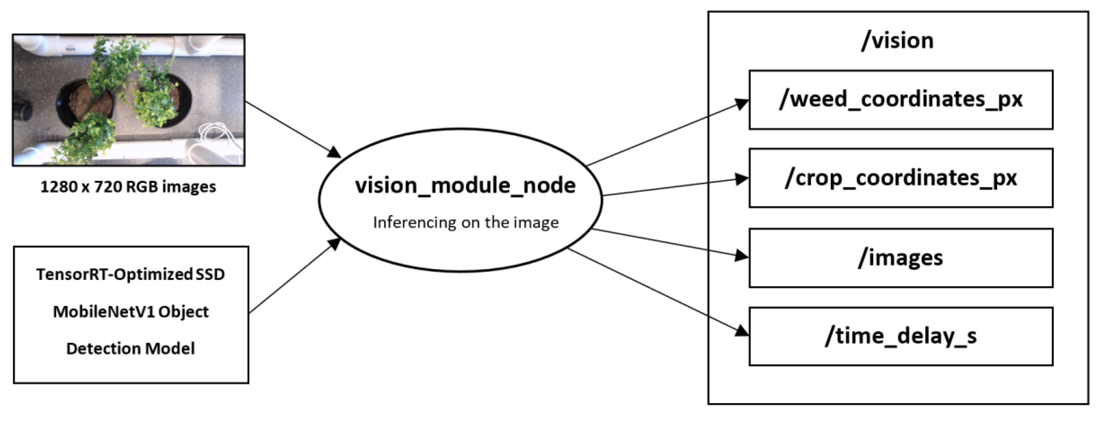
To enable modularity, the software framework, as illustrated in Figure 5, was also implemented using ROS version Melodic Morenia, which was the version that was compatible with Ubuntu 18.04. A node is a virtual representation of a component that can send or receive messages directly from other nodes. The vision module or node required two inputs: (1) RGB video stream from a video capture device and (2) TensorRT-optimized SSD MobileNetV1 object detection model. It calculates and outputs four parameters, namely: (1) weed coordinates, (2) crop coordinates, (3) processed images, and (4) total delay time. Each parameter was published into its respective topics. Table 4 summarizes the datatype and the function of these outputs.
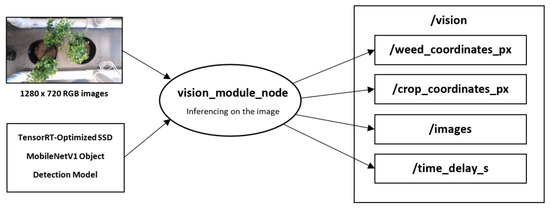
Figure 5.
Software framework of the vision module.
Table 4.
Output parameters of the vision module with their description.
2.6.2. Dataset Preparation and Training of the CNN Model
Using the Jetson Inference library, a CNN model for plant detection was trained using SSD MobileNetV1 object detection architecture and PyTorch machine learning framework. A total of 2000 sample images of artificial potted plants at 1280 × 720 composed of 50% weeds and 50% plants were prepared. For CNN model training and validation, 80% and 20% of the datasets were used, respectively. A batch size of 4, base learning rate of 0.001, and momentum of 0.90 were used to train the model for 100 epochs (5000 iterations).
2.6.3. Testing and Simulation
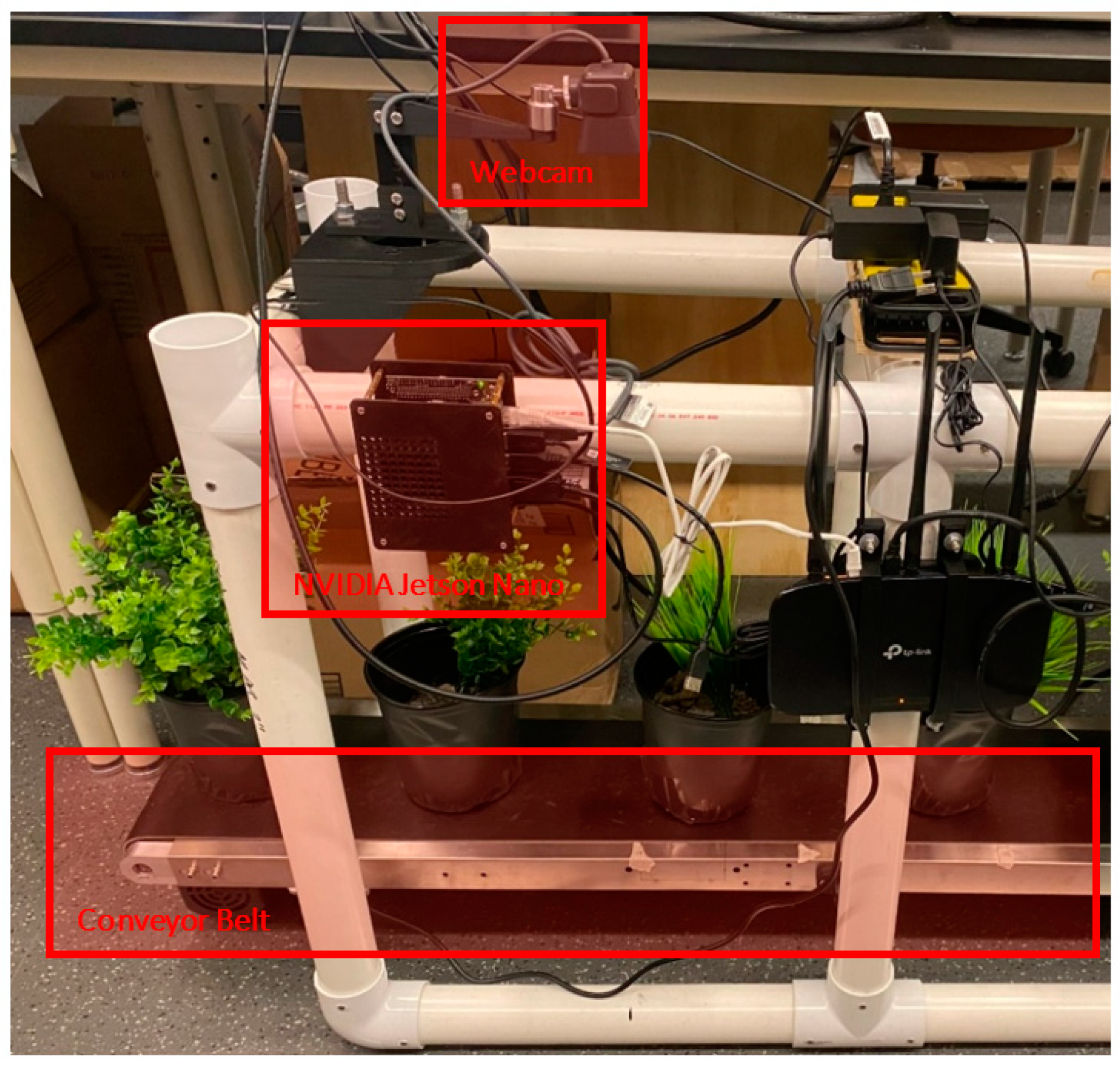
The performance requirement for the vision module was to avoid missed detections for spraying operations at walking speeds, which was 0.1 m/s at minimum [35,36,37]. The Jetson Nano and webcam were mounted at a height where was equal to 0.79 m, as shown in Figure 6. was determined so that the top projections of the potted plants were within the camera frame, and the camera and plants would not collide during motion. A conveyor belt equipped with a variable speed motor was used to reproduce the relative travel velocity of the vision system at 0.1, 0.2, and 0.3 m/s. A maximum of 0.3 m/s was used, since beyond this conveyor speed consistent at 0.2 m was difficult to achieve, even with three people performing the manual loading and unloading, as the potted artificial plants were traveling too fast.

Figure 6.
Laboratory setup composed of Jetson Nano 4GB, Logitech StreamCam Plus, and variable speed conveyor belt with artificial potted plants.
A total of 60 potted plants were loaded onto the conveyor for each conveyor speed setting. Detection was carried out at a minimum conference threshold of 0.5. Detected and correctly classified plants were considered true positives (TP), while detected and incorrectly classified plants were categorized as false positives (FP). Missed detections were classified as false negatives (FN). The precision () and recall () of the vision module were then determined using Equations (15) and (16), respectively.
3. Results and Discussion
The sensitivity of and to the total traversed distance was first determined to establish the that was used in the experimental design. The influence of and at specific on and were then compared and analyzed. Finally, the results of performance testing the vision module were compared to theoretical and simulation results.
3.1. Sensitivity Analysis
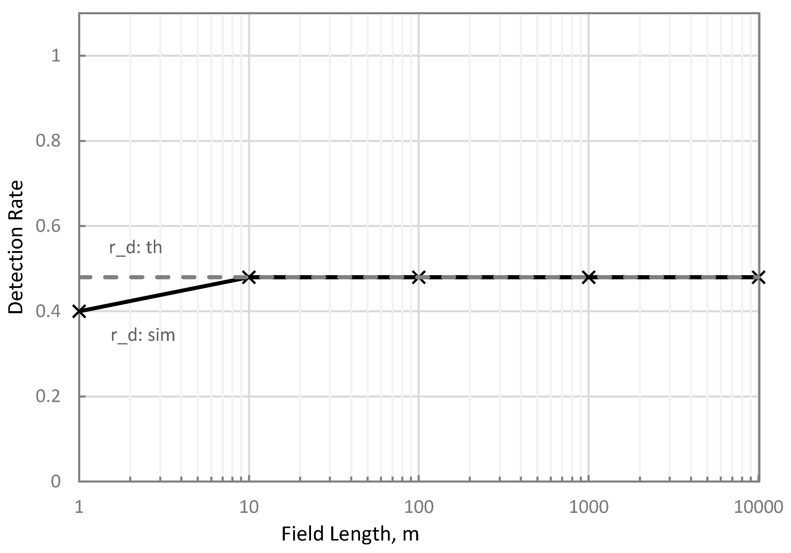
As illustrated in Figure 7, the sensitivity analysis results showed that and converged at 10 m traversed distance. The 20% difference of from can be attributed to the different variables considered to determine each parameter. used inferencing speed, travel velocity, and capture width to theoretically calculate the gaps between consecutive processed frames related to the detection rate, as illustrated in Section 2.1.
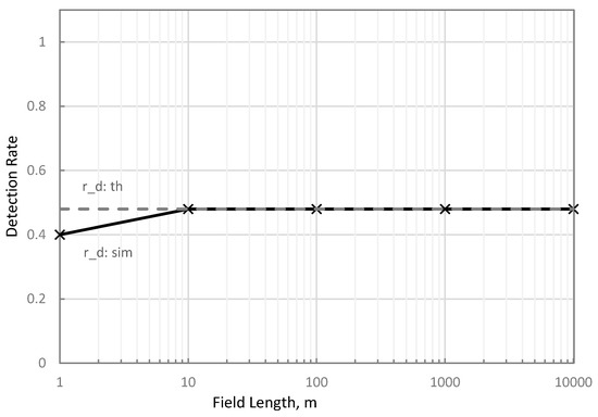
Figure 7.
Theoretical (solid) and simulated (broken-line) detection rates at 1, 10, 100, 1000, and 10,000 m field lengths at 0.2 m hill spacing, 2travel velocity, , and 0.5 m frame capture width.
On the other hand, determined the detection rate based on the number of unique plants within the processed frames, as influenced by traversed distance, hill spacing, inferencing speed, travel velocity, and capture width, as described in Section 2.2, Section 2.3, Section 2.4. Results showed that simulation better approximated the detection rate than theoretical approaches at less than 10 m traversed distance, 0.2 m hill spacing, 2.5 m/s travel velocity, 2.4 fps, and 0.5 m frame capture width.
These results infer that at very short distances, approximates the detection rate more accurately than . However, for long traversed distances, the influence of hill spacing on the detection rate was no longer significant and can simply be used to calculate the detection rate.
3.2. Effects of and
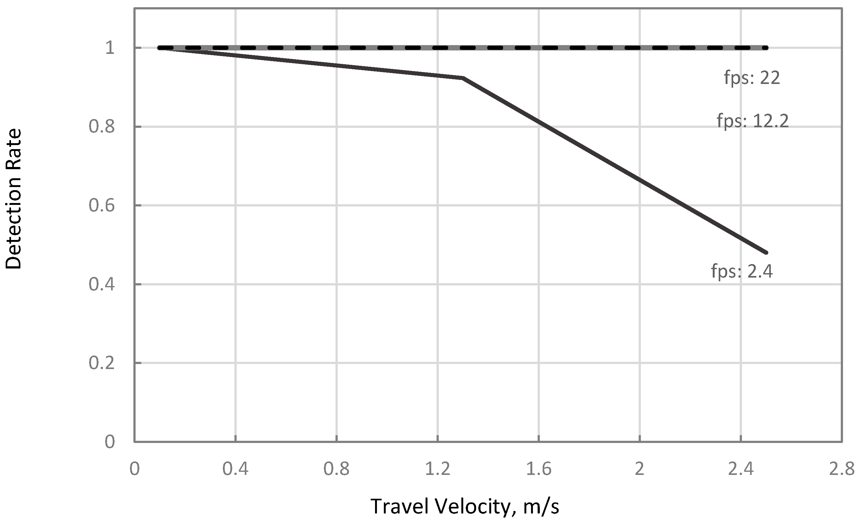
Table 5 summarizes the theoretical and simulation results on the combinations of and at equal to 0.5-m. Comparing the to for any combinations of the tested parameters showed that detection rates were equal. Results also showed that there were no missed detections at any when the inferencing speeds were at 12.2 and 22 fps (Case 2), as illustrated in Figure 8 and Figure 9. These results infer that one-stage object detection models, such as YOLO and SSD, running on a discrete GPU such as 1070TI, have sufficient inferencing speed to avoid detection gaps in typical ranges of travel velocities for agricultural field operations. The result was also comparable to the 92% precision of the CNN-based MVS with 22 fps inferencing speed in the study of Partel et al. (2019) [11]. Therefore, these results infer that using a one-stage CNN model such as YOLOv3 on a laptop with NVIDIA 1070TI GPU or better can provide sufficient inferencing speed to avoid gaps in different field operations. However, as mentioned in Section 1, the study did not report the travel velocity and field of view length of their setup. Thus, only an estimated performance comparison can be made.
Table 5.
Theoretical and simulation performance of a vision system for plant detection at at three-levels of travel velocity ( ) and inferencing speed ( ).
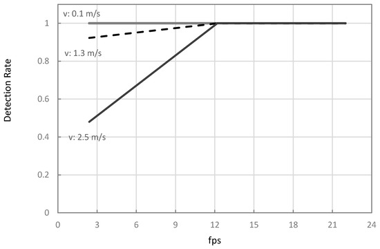
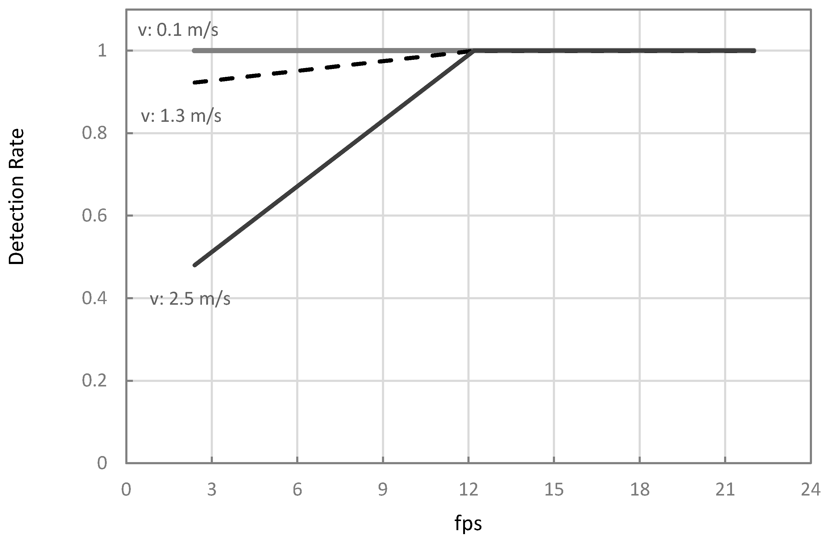
Figure 8.
Simulated plant hill detection rates of the vision system moving at 0.1, 1.3, and 2.5 m/s at different inferencing speeds ().
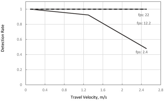
Figure 9.
Simulated plant hill detection rates of the vision system moving at 2.4, 12.2, and 22 fps at different travel velocities.
The result of this study also agrees with the results of other studies with known , , and . In the study of Chechliński et al. (2019) [23], their CNN-based-vision spraying system had , , and . Applying these values to Equation (2) also yields (Case 2), which correctly predicted their results of full-field coverage. In the study of Esau et al. (2018) [10], their vision-based spraying system had , , and and also falls under Case 2. Similarly, the vision-based robotic fertilizer application in the study of Chattha et al. (2018) [13] had a , , and . Again, calculating yielded Case 2, which also agrees with their results.
At 2.4 fps, the simulated MVS failed to detect some plant hills when was 1.3 (Treatment 4) or 2.4 m/s (Treatment 7). In contrast, missed detections were absent at 0.1 m/s (Treatment 1). As mentioned in Section 2.5, treatments 1, 4, and 7 represent typical inferencing speeds of CNN models, such as YOLOv3 running in an embedded system, such as NVIDIA TX2 [11]. From these results, it can be inferred that unless CNN object detection models were optimized, such as illustrated in previous studies [23,45], MVS with embedded systems shall only be applicable for agricultural field operations at walking speeds.
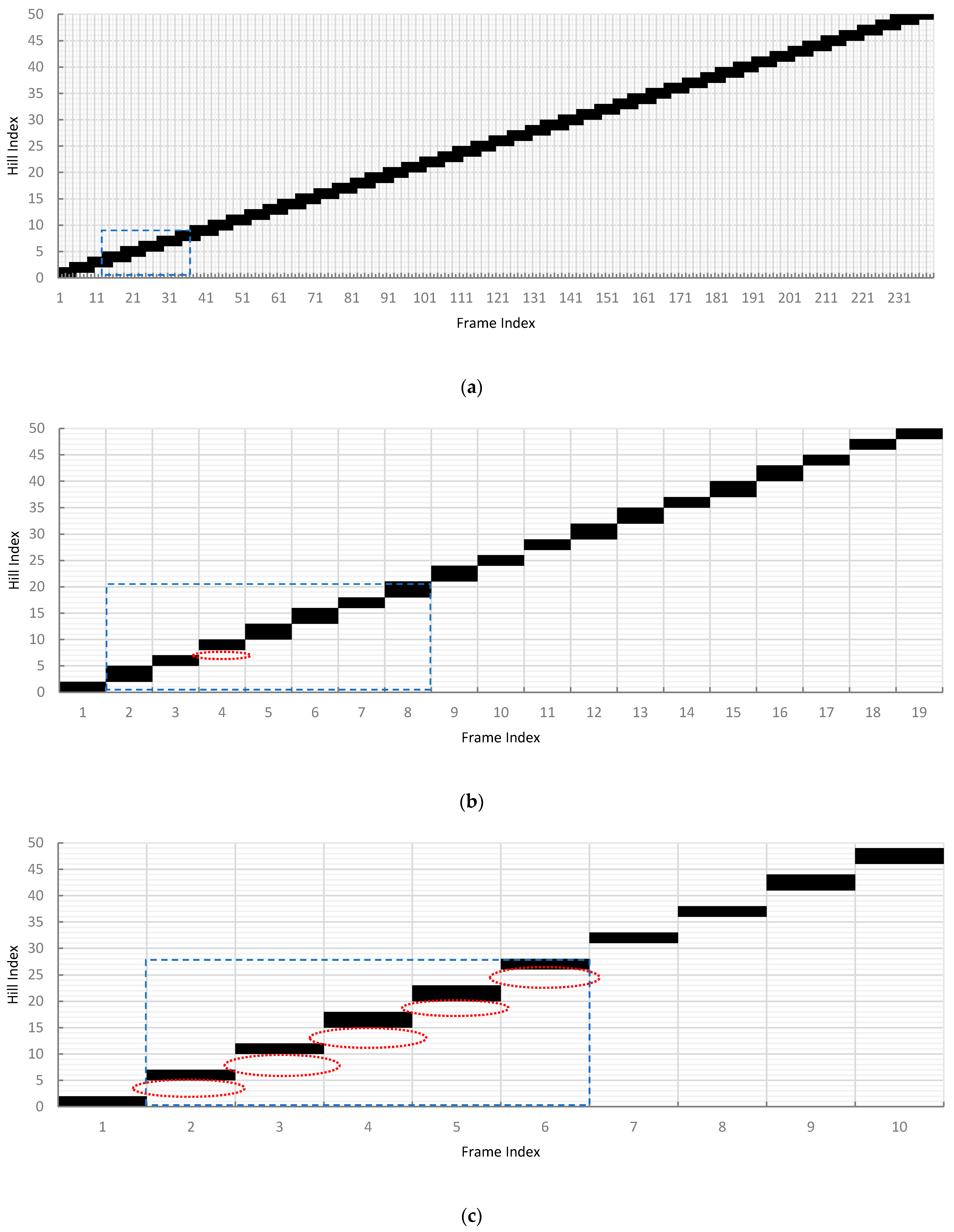
Figure 10 illustrates the detected hills per camera frame along the first 10 m traversed distance of treatments simulated at 2.4 fps (Treatments 1, 4, and 7). From Figure 10, three information can be obtained: (1) absence of vertical gaps between consecutive frames; (2) horizontal overlaps among consecutive frames; and (3) detection pattern. In Figure 10a, the absence of vertical gaps at 0.1 m/s detections infers that all the hills were detected as the vision moved along the field length. The horizontal overlaps among consecutive frames also illustrate that a plant hill was captured by more than one processed frame. Finally, a detection pattern was observed to repeat every 24 consecutive frames or approximately every 1 m length. The length of the pattern was calculated by multiplying the number of frames to complete a cycle and .
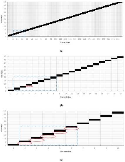
Figure 10.
Range of plant hill indices that were detected per frame along the first 10 m of the simulated field at 2.4 fps, 0.5 m capture width, 0.2 m hill spacing at (a) 0.1 m/s, (b) 1.3 m/s, and (c) 2.5 m/s. Blue broken lines enclose a detection pattern, while broken red lines specify the missed plant hills.
In contrast, the vertical gaps in some consecutive frames at 1.3 m/s, shown in Figure 10b, illustrated the missed detections. Horizontal overlaps were also absent. Hence, the detected plant hills were only represented in the frame once. The vision module traveled too fast and processed the captured frame too slowly at the set capture width, as demonstrated by the detection pattern of one missed plant hill every seven consecutive frames or approximately every 3.8 m traversed distance.
Similar results were also observed at 2.5 m/s travel velocity, as shown in Figure 10c. However, the vertical gaps were more extensive than Figure 10b due to faster travel speed. Observing the detection pattern showed that 14 plant hills were being undetected by the vision system every five frames or approximately every 5.21 m traversed distance. This pattern that forms every 5.21 m further explains the difference in the and in the sensitivity analysis in Section 3.1, when the traversed distance was only 1 m. A complete detection pattern was already formed when the distance was more than 10 m, resulting in better detection rate estimates.
From these results, two vital insights can be drawn. First, at , shall have a margin of error when the length of the detection pattern is less than the traversed distance. Second, concerning future studies, object tracking algorithms, such as Euclidean-distance-based tracking [46], that requires objects should be present in at least two frames, would be not applicable when . Hence, the importance that in MVS designs is further emphasized.
3.3. Effect of Increasing S or Multiple Cameras
In cases where (Case 3), a practical solution to increase is to raise the camera mounting height, which, in effect, shall increase . However, if raising the camera mounting height is inappropriate as doing so shall also decrease object details, the use of multiple cameras can be a viable solution.
Figure 11 illustrates the effect of increasing the effective or using multiple cameras on the calculated values of for the three levels of infencing speeds (2.4, 12.2, and 22 fps) simulated at . The results showed that treatments with missed detections exceeded the allowable . For treatments 4 and 7, the allowable travel velocity was only 1.2 m/s using a single camera module, which was less than the simulated of 1.3 and 2.5 m/s, respectively.
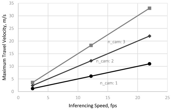
Figure 11.
Theoretical maximum travel velocity to prevent missed detections with 1, 2, and 3 cameras at 2.4, 12.2, and 22.0 fps.
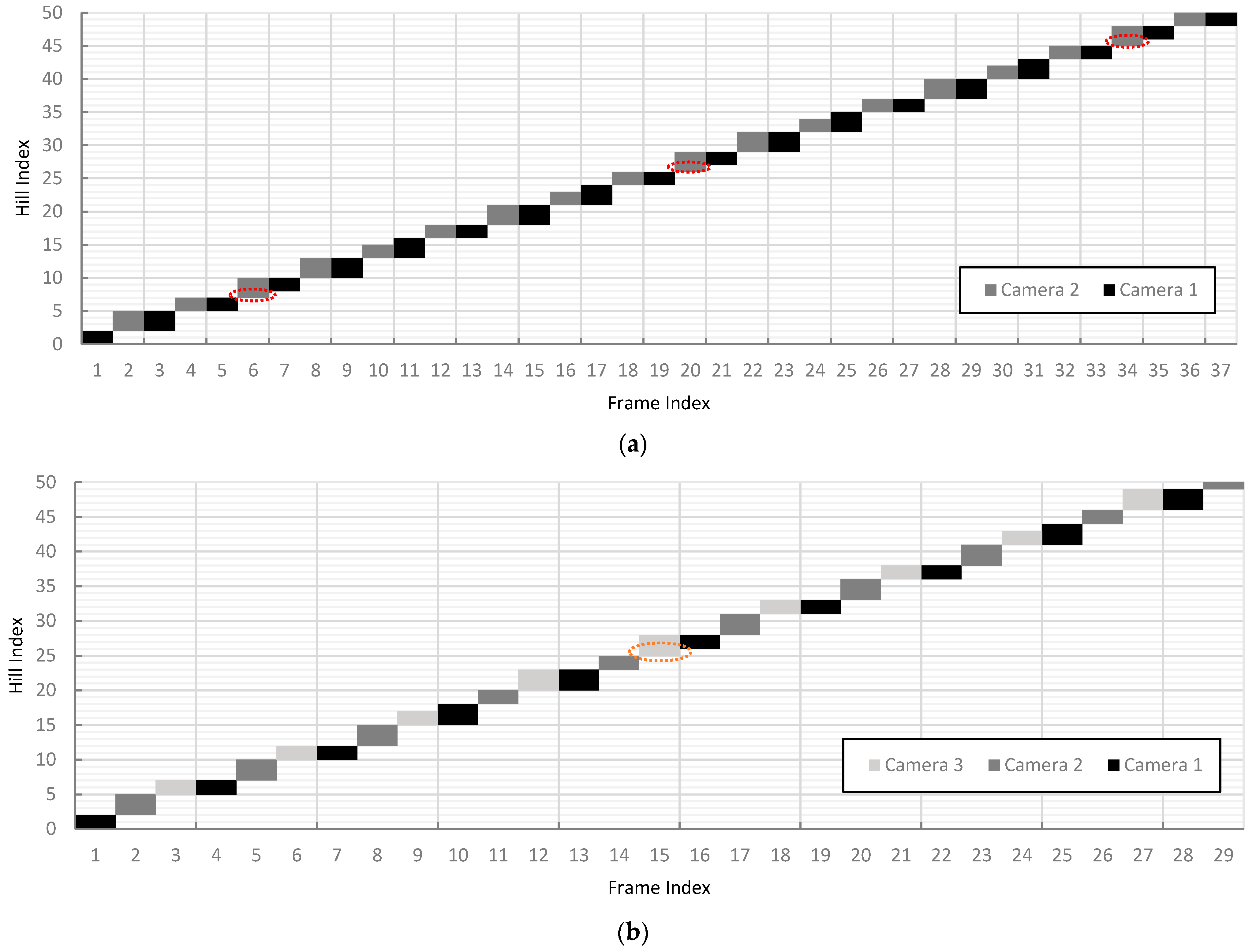
Calculating using Equation (6) for treatments 4 and 7 showed that 2 and 3 vision modules, respectively, were required to prevent missed detections. Thus, using two vision modules for treatment 4 prevented missed detections, as shown in Figure 12. The 6th, 20th, and 34th frames captured by the second camera detected the plants undetected by the first camera.
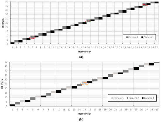
Figure 12.
The range of plant hill indices detected per frame along the first 10 m of the simulated field at , , and : (a) detections at 1.3 m/s using two cameras where broken red lines represent plant hills undetected by the first camera but detected by the second camera; and (b) detections at 2.5 m/s and three cameras where broken orange lines represent plant hills undetected by the first and second cameras but detected by the third camera.
As predicted, a two-vision-module configuration for treatment 7 was insufficient in preventing missed detections since the simulated of 2.5 m/s of the vision system was still higher than the increased . As illustrated in Figure 12, without a third camera, the two-camera configuration would still result in an undetected hill on the 16th frame.
Based on these simulated results, the problem of missed detection due to the slow inferencing speed of embedded systems could be potentially solved by using multiple, adjacent, non-overlapping, and colinear cameras along the traversed row when raising the height of the camera was unwanted.
3.4. Vision Module Simulation and Testing Performance
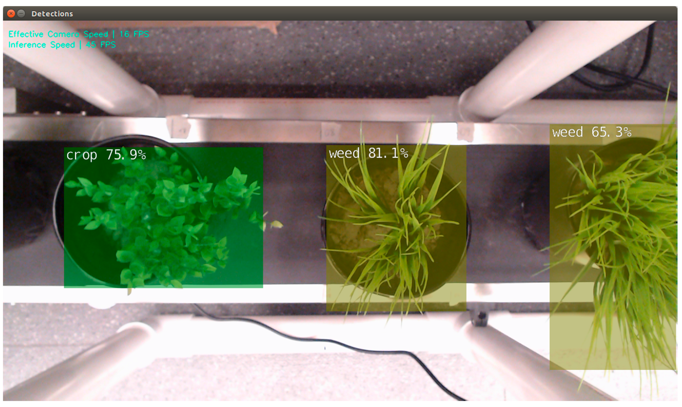
Figure 13 shows the sample detection of the vision module. Results showed that using a TensorRT-optimized SSD MobileNetV1 to detect plants in 1280 × 720 images on an NVIDIA Jetson Nano 4 GB had an average inferencing speed of 45 fps. This average inferencing speed only represented the elapsed time to inference on an already loaded frame. However, due to calculation overheads caused by additional data processing and transmission, the average effective inferencing speed of the vision module was only 16 fps, as shown in Figure 13. The effective speed was the average time difference for the vision module to complete a single loop, including grabbing a frame from the camera, inferencing, calculating detection parameters, image processing, and transmitting data.
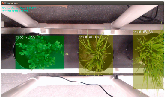
Figure 13.
Sample real-time inferencing using trained SSD MobileNetV1 model and optimized in TensorRT. The vision system utilized Jetson Inference API.
The results using the theoretical approach and simulation for the vision module are shown in Table 6. Using Equation (2), the configuration of the laboratory setup falls under Case 2 since . Then, using Equation (4), was calculated to be equal to 1.00. Applying Equation (5) yields , which was highly sufficient for the target 0.3 m/s and inferred that multiple vision modules were not required to prevent missed detections. Theoretical prediction of the performance of the vision module showed that the configuration was sufficient to prevent missed detection. Likewise, the theoretical result was confirmed by the simulation results that showed no missed detections () for both crops and weeds among the simulated .
Table 6.
Theoretical and simulation performance of the CNN-based vision module for plant detection at , 16, and at three-levels of travel velocity ( ).
Table 7 summarizes the precision and recall of the trained CNN model in detecting potted plants at different relative travel velocities of the conveyor. Results showed that the combination of an optimized SSD MobileNetV1 in TensorRT running in a Jetson Nano 4 GB have robust detection performance, and incorrect or missed detections were absent despite increasing travel velocity. Comparing the value of to and , results showed that the detection rates were equal. The recall was used for comparison instead of precision since the former is the ratio of the correctly detected plants to the total sample plants. This definition of in Equation (16) is equivalent to the definition of in Equation (14). Since the , and were equal, these results proved the validity of the theoretical concepts and simulation methods presented in this study. Hence, and can be used to theoretically determine the detection rate of a vision system in capturing plant images as a function of and with known .
Table 7.
The detection performance of the CNN-based vision module for detecting a 60 potted plants at different conveyor velocities ( ).
4. Conclusions
This study presented a practical approach to quantify and aid in the development of a CNN-based vision module through the introduction of the dimensionless parameter . The reliability of in predicting the of an MVS as a function of inferencing speed and travel velocity was successfully demonstrated by having no margin of error compared to simulated and actual MVS at sufficient traversed distance (≥10 m). In addition, a set of scripts for simulating the performance of a vision system for plant detection was also developed and showed no margin of error compared to the of actual MVS. This set of scripts was made publicly available to verify the results of this study and provide a practical tool for developers in optimizing design configurations of a vision-based plant detection system.
The mechanism of missed detection was also successfully illustrated by evaluating each of the simulated frames in detail. Using the concept of , simulation, and detailed assessment of each processed frame, the mechanism to prevent missed plant hills by increasing the effective through synchronous multi-camera vision systems in low-frame processing rate hardware was also successfully presented.
Furthermore, a vision module was also successfully developed and tested. Performance testing showed that the and accurately predicted the of the vision module with no margin of error. The script for the vision module was also made available in a public repository where future improvements shall also be uploaded.
However, despite accomplishing the set objectives in this research, the study encountered limitations that shall be improved in future research. First, the robustness of in predicting the detection rate was supported mainly by simulation data. The current laboratory tests were only implemented at a maximum travel velocity of 0.3 m/s due to limitations in the manual loading of the test plants. At this time, the study relied on results of other studies to validate the robustness of at higher travel velocities and different inferencing speeds. Thus, the concepts presented in this shall be further tested to determine the robustness of at higher travel velocities during the application of the developed vision module on actual field scenarios.
Lastly, the methodology to calculate and assumed that the CNN has 100% precision. In cases less than 100% precision, it can be theorized that and can be multiplied by the precision of the CNN to estimate the effective recall of a CNN-based vision system in evaluating moving objects across the camera frame. However, this concept is yet to be demonstrated and shall also be included in future studies.
Author Contributions
Conceptualization, P.R.S.; methodology, P.R.S. and H.Z.; software, P.R.S.; validation, P.R.S.; formal analysis, P.R.S. and H.Z.; investigation, P.R.S. and H.Z.; resources, P.R.S. and H.Z.; data curation, P.R.S.; writing—original draft preparation, P.R.S.; writing—review and editing, H.Z.; visualization, P.R.S.; supervision, H.Z.; project administration, H.Z.; funding acquisition, P.R.S. and H.Z. All authors have read and agreed to the published version of the manuscript.
Funding
This research received no external funding.
Institutional Review Board Statement
Not applicable.
Informed Consent Statement
Not applicable.
Data Availability Statement
The scripts used in the simulation and vision module were made publicly available in GitHub under BSD license to use, test, and validate the data presented in this study. The scripts for simulation are available at https://github.com/paoap/vision-module-simulation, (accessed on 31 December 2021) while the vision module software framework can be downloaded from https://github.com/paoap/plant-detection-vision-module (accessed on 31 December 2021).
Conflicts of Interest
The authors declare no conflict of interest.
References
- Pelzom, T.; Katel, O. Youth Perception of Agriculture and Potential for Employment in the Context of Rural Development in Bhutan. Dev. Environ. Foresight 2017, 3, 2336–6621. [Google Scholar]
- Mortan, M.; Baciu, L. A Global Analysis of Agricultural Labor Force. Manag. Chall. Contemp. Soc. 2016, 9, 57–62. [Google Scholar]
- Priyadarshini, P.; Abhilash, P.C. Policy Recommendations for Enabling Transition towards Sustainable Agriculture in India. Land Use Policy 2020, 96, 104718. [Google Scholar] [CrossRef]
- Rose, D.C.; Sutherland, W.J.; Barnes, A.P.; Borthwick, F.; Ffoulkes, C.; Hall, C.; Moorby, J.M.; Nicholas-Davies, P.; Twining, S.; Dicks, L.V. Integrated Farm Management for Sustainable Agriculture: Lessons for Knowledge Exchange and Policy. Land Use Policy 2019, 81, 834–842. [Google Scholar] [CrossRef]
- Lungarska, A.; Chakir, R. Climate-Induced Land Use Change in France: Impacts of Agricultural Adaptation and Climate Change Mitigation. Ecol. Econ. 2018, 147, 134–154. [Google Scholar] [CrossRef] [Green Version]
- Thorp, K.R.; Tian, L.F. A Review on Remote Sensing of Weeds in Agriculture. Precis. Agric. 2004, 5, 477–508. [Google Scholar] [CrossRef]
- Bechar, A.; Vigneault, C. Agricultural Robots for Field Operations: Concepts and Components. Biosyst. Eng. 2016, 149, 94–111. [Google Scholar] [CrossRef]
- Aravind, K.R.; Raja, P.; Pérez-Ruiz, M. Task-Based Agricultural Mobile Robots in Arable Farming: A Review. Span. J. Agric. Res. 2017, 15, e02R01. [Google Scholar] [CrossRef]
- Tian, H.; Wang, T.; Liu, Y.; Qiao, X.; Li, Y. Computer Vision Technology in Agricultural Automation—A Review. Inf. Process. Agric. 2020, 7, 1–19. [Google Scholar] [CrossRef]
- Esau, T.; Zaman, Q.; Groulx, D.; Farooque, A.; Schumann, A.; Chang, Y. Machine Vision Smart Sprayer for Spot-Application of Agrochemical in Wild Blueberry Fields. Precis. Agric. 2018, 19, 770–788. [Google Scholar] [CrossRef]
- Partel, V.; Charan Kakarla, S.; Ampatzidis, Y. Development and Evaluation of a Low-Cost and Smart Technology for Precision Weed Management Utilizing Artificial Intelligence. Comput. Electron. Agric. 2019, 157, 339–350. [Google Scholar] [CrossRef]
- Wang, A.; Zhang, W.; Wei, X. A Review on Weed Detection Using Ground-Based Machine Vision and Image Processing Techniques. Comput. Electron. Agric. 2019, 158, 226–240. [Google Scholar] [CrossRef]
- Chattha, H.S.; Zaman, Q.U.; Chang, Y.K.; Read, S.; Schumann, A.W.; Brewster, G.R.; Farooque, A.A. Variable Rate Spreader for Real-Time Spot-Application of Granular Fertilizer in Wild Blueberry. Comput. Electron. Agric. 2014, 100, 70–78. [Google Scholar] [CrossRef]
- Zujevs, A.; Osadcuks, V.; Ahrendt, P. Trends in Robotic Sensor Technologies for Fruit Harvesting: 2010–2015. Procedia Comput. Sci. 2015, 77, 227–233. [Google Scholar] [CrossRef]
- Tang, Y.; Chen, M.; Wang, C.; Luo, L.; Li, J.; Lian, G.; Zou, X. Recognition and Localization Methods for Vision-Based Fruit Picking Robots: A Review. Front. Plant Sci. 2020, 11, 510. [Google Scholar] [CrossRef]
- Liu, B.; Bruch, R. Weed Detection for Selective Spraying: A Review. Curr. Robot. Rep. 2020, 1, 19–26. [Google Scholar] [CrossRef] [Green Version]
- Jha, K.; Doshi, A.; Patel, P.; Shah, M. A Comprehensive Review on Automation in Agriculture Using Artificial Intelligence. Artif. Intell. Agric. 2019, 2, 1–12. [Google Scholar] [CrossRef]
- Huang, J.; Rathod, V.; Sun, C.; Zhu, M.; Korattikara, A.; Fathi, A.; Fischer, I.; Wojna, Z.; Song, Y.; Guadarrama, S.; et al. Speed/Accuracy Trade-Offs for Modern Convolutional Object Detectors. In Proceedings of the 2017 IEEE Conference on Computer Vision and Pattern Recognition (CVPR), Honolulu, HI, USA, 21–26 July 2017; IEEE: New York, NY, USA, 2017; Volume 84, pp. 3296–3297. [Google Scholar]
- Kamilaris, A.; Prenafeta-Boldú, F.X. A Review of the Use of Convolutional Neural Networks in Agriculture. J. Agric. Sci. 2018, 156, 312–322. [Google Scholar] [CrossRef] [Green Version]
- Cecotti, H.; Rivera, A.; Farhadloo, M.; Pedroza, M.A. Grape Detection with Convolutional Neural Networks. Expert Syst. Appl. 2020, 159, 113588. [Google Scholar] [CrossRef]
- Jia, W.; Tian, Y.; Luo, R.; Zhang, Z.; Lian, J.; Zheng, Y. Detection and Segmentation of Overlapped Fruits Based on Optimized Mask R-CNN Application in Apple Harvesting Robot. Comput. Electron. Agric. 2020, 172, 105380. [Google Scholar] [CrossRef]
- Olsen, A.; Konovalov, D.A.; Philippa, B.; Ridd, P.; Wood, J.C.; Johns, J.; Banks, W.; Girgenti, B.; Kenny, O.; Whinney, J.; et al. DeepWeeds: A Multiclass Weed Species Image Dataset for Deep Learning. Sci. Rep. 2019, 9, 2058. [Google Scholar] [CrossRef] [PubMed]
- Chechliński, Ł.; Siemiątkowska, B.; Majewski, M. A System for Weeds and Crops Identification—Reaching over 10 fps on Raspberry Pi with the Usage of MobileNets, DenseNet and Custom Modifications. Sensors 2019, 19, 3787. [Google Scholar] [CrossRef] [PubMed] [Green Version]
- Liu, J.; Abbas, I.; Noor, R.S. Development of Deep Learning-Based Variable Rate Agrochemical Spraying System for Targeted Weeds Control in Strawberry Crop. Agronomy 2021, 11, 1480. [Google Scholar] [CrossRef]
- Hussain, N.; Farooque, A.; Schumann, A.; McKenzie-Gopsill, A.; Esau, T.; Abbas, F.; Acharya, B.; Zaman, Q. Design and Development of a Smart Variable Rate Sprayer Using Deep Learning. Remote Sens. 2020, 12, 4091. [Google Scholar] [CrossRef]
- Villette, S.; Maillot, T.; Guillemin, J.P.; Douzals, J.P. Simulation-Aided Study of Herbicide Patch Spraying: Influence of Spraying Features and Weed Spatial Distributions. Comput. Electron. Agric. 2021, 182, 105981. [Google Scholar] [CrossRef]
- Wang, H.; Hohimer, C.J.; Bhusal, S.; Karkee, M.; Mo, C.; Miller, J.H. Simulation as a Tool in Designing and Evaluating a Robotic Apple Harvesting System. IFAC-PapersOnLine 2018, 51, 135–140. [Google Scholar] [CrossRef]
- Lehnert, C.; Tsai, D.; Eriksson, A.; McCool, C. 3D Move to See: Multi-Perspective Visual Servoing towards the next Best View within Unstructured and Occluded Environments. In Proceedings of the 2019 IEEE/RSJ International Conference on Intelligent Robots and Systems (IROS), Macau, China, 3–8 November 2019; IEEE: New York, NY, USA, 2019; pp. 3890–3897. [Google Scholar]
- Korres, N.E.; Burgos, N.R.; Travlos, I.; Vurro, M.; Gitsopoulos, T.K.; Varanasi, V.K.; Duke, S.O.; Kudsk, P.; Brabham, C.; Rouse, C.E.; et al. New Directions for Integrated Weed Management: Modern Technologies, Tools and Knowledge Discovery. In Advances in Agronomy; Elsevier Inc.: Amsterdam, The Netherlands, 2019; Volume 155, pp. 243–319. ISBN 9780128174081. [Google Scholar]
- Hajjaj, S.S.H.; Sahari, K.S.M. Review of Agriculture Robotics: Practicality and Feasibility. In Proceedings of the 2016 IEEE International Symposium on Robotics and Intelligent Sensors (IRIS), Tokyo, Japan, 17–20 December 2016; pp. 194–198. [Google Scholar]
- Gauss, L.; Lacerda, D.P.; Sellitto, M.A. Module-Based Machinery Design: A Method to Support the Design of Modular Machine Families for Reconfigurable Manufacturing Systems. Int. J. Adv. Manuf. Technol. 2019, 102, 3911–3936. [Google Scholar] [CrossRef]
- Brunete, A.; Ranganath, A.; Segovia, S.; de Frutos, J.P.; Hernando, M.; Gambao, E. Current Trends in Reconfigurable Modular Robots Design. Int. J. Adv. Robot. Syst. 2017, 14, 172988141771045. [Google Scholar] [CrossRef] [Green Version]
- Lu, Y.; Young, S. A Survey of Public Datasets for Computer Vision Tasks in Precision Agriculture. Comput. Electron. Agric. 2020, 178, 105760. [Google Scholar] [CrossRef]
- Iñigo-Blasco, P.; Diaz-del-Rio, F.; Romero-Ternero, M.C.; Cagigas-Muñiz, D.; Vicente-Diaz, S. Robotics Software Frameworks for Multi-Agent Robotic Systems Development. Robot. Auton. Syst. 2012, 60, 803–821. [Google Scholar] [CrossRef]
- Spencer, J.; Dent, D.R. Walking Speed as a Variable in Knapsack Sprayer Operation: Perception of Speed and the Effect of Training. Trop. Pest Manag. 1991, 37, 321–323. [Google Scholar] [CrossRef]
- Gatot, P.; Anang, R. Liquid Fertilizer Spraying Performance Using A Knapsack Power Sprayer On Soybean Field. IOP Conf. Ser. Earth Environ. Sci. 2018, 147, 012018. [Google Scholar] [CrossRef]
- Cerruto, E.; Emma, G.; Manetto, G. Spray applications to tomato plants in greenhouses. Part 1: Effect of walking direction. J. Agric. Eng. 2009, 40, 41. [Google Scholar] [CrossRef] [Green Version]
- Rasmussen, J.; Azim, S.; Nielsen, J.; Mikkelsen, B.F.; Hørfarter, R.; Christensen, S. A New Method to Estimate the Spatial Correlation between Planned and Actual Patch Spraying of Herbicides. Precis. Agric. 2020, 21, 713–728. [Google Scholar] [CrossRef]
- Arvidsson, T.; Bergström, L.; Kreuger, J. Spray Drift as Influenced by Meteorological and Technical Factors. Pest Manag. Sci. 2011, 67, 586–598. [Google Scholar] [CrossRef]
- Dou, H.; Zhai, C.; Chen, L.; Wang, S.; Wang, X. Field Variation Characteristics of Sprayer Boom Height Using a Newly De-signed Boom Height Detection System. IEEE Access 2021, 9, 17148–17160. [Google Scholar] [CrossRef]
- Holterman, H.J.; van de Zande, J.C.; Porskamp, H.A.J.; Huijsmans, J.F.M. Modelling Spray Drift from Boom Sprayers. Com-Puter. Electron. Agric. 1997, 19, 1–22. [Google Scholar] [CrossRef]
- Yinyan, S.; Zhichao, H.; Xiaochan, W.; Odhiambo, M.O.; Weimin, D. Motion Analysis and System Response of Fertilizer Feed Apparatus for Paddy Variable-Rate Fertilizer Spreader. Comput. Electron. Agric. 2018, 153, 239–247. [Google Scholar] [CrossRef]
- Machleb, J.; Peteinatos, G.G.; Sökefeld, M.; Gerhards, R. Sensor-Based Intrarow Mechanical Weed Control in Sugar Beets with Motorized Finger Weeders. Agronomy 2021, 11, 1517. [Google Scholar] [CrossRef]
- Fennimore, S.A.; Cutulle, M. Robotic Weeders Can Improve Weed Control Options for Specialty Crops. Pest Manag. Sci. 2019, 75, 1767–1774. [Google Scholar] [CrossRef]
- Pinto de Aguiar, A.S.; Neves dos Santos, F.B.; Feliz dos Santos, L.C.; de Jesus Filipe, V.M.; Miranda de Sousa, A.J. Vineyard Trunk Detection Using Deep Learning—An Experimental Device Benchmark. Comput. Electron. Agric. 2020, 175, 105535. [Google Scholar] [CrossRef]
- Qian, X.; Han, L.; Wang, Y.; Ding, M. Deep Learning Assisted Robust Visual Tracking with Adaptive Particle Filtering. Signal Processing Image Commun. 2018, 60, 183–192. [Google Scholar] [CrossRef]

Publisher’s Note: MDPI stays neutral with regard to jurisdictional claims in published maps and institutional affiliations. |
© 2022 by the authors. Licensee MDPI, Basel, Switzerland. This article is an open access article distributed under the terms and conditions of the Creative Commons Attribution (CC BY) license (https://creativecommons.org/licenses/by/4.0/).