Abstract
The stepless flow control system offers important energy-saving technology for reciprocating compressors in the petrochemical and oil refining industries. Optimizing the movement characteristics of the unloader and suction valve is vital to improving the energy-saving level of the system and reducing the overall operating cost. However, the system has many of the characteristics of multi-system coupling and multi-parameter crossover; thus, it is difficult to optimize the key control parameters. In this study, to optimize the system inlet pressure, return pressure, and return spring stiffness parameters, a working model of the flow control system based on multi-system coupling was established. Using the ejection and withdrawal speeds of the unloader, the flow displacement deviation, and the gas work deviation of the control system as the optimization parameters, we used the response surface method to establish an optimization proxy model between the objective function and key parameters. Additionally, verification of the model’s accuracy and sensitivity analyses were completed. Finally, a double optimization scheme based on a non-dominated genetic algorithm (NSGA-II) was proposed. Simulation and experimental results show that with optimization of the return spring, oil inlet pressure, and oil return pressure, the unloader’s kinematic characteristics were also optimized at full load. The impact energy of the ejector and withdrawal speed of the unloader were reduced, and the compressor flow control error was less than 5%, which effectively improved the comprehensive working performance of the stepless flow control system.
1. Introduction
Large-scale reciprocating compressors are widely used in fields such as oil refining, the chemical industry, and natural gas transportation. During operation, the flow of a compressor must be adjusted according to changes in the process requirements [1]. Stepless flow control systems, based on the reflux of the suction valve, are widely used because of their wide adjustment range and small pressure fluctuation at the back end, which saves a significant amount of energy for the compressor [2]. However, because the system changes the dynamic behavior and gas flow characteristics of the valve, the compressor deviates from the normal design conditions, resulting in an increase in the valve failure rate [3]. As an important part of the compressor, the valve’s motion characteristics directly affect the operating efficiency and reliability of the compressor [4]. Tang [5] observed that the movement characteristics of a valve can be controlled by changing the key parameters of the unloader. Therefore, optimizing the parameters affecting the unloader and the system process parameters is vital to extending the service life of the valve and reducing the operating cost of the compressor.
The stepless flow control system of a reciprocating compressor, based on the operating principle of the top-opening suction valve, is primarily composed of a mechanical system, an electronic control system, a hydraulic system, and the gas system of the compressor. Coupling and parameter interactions exist between the subsystems. The suction valve is the coupling point between the mechanical and compressor gas systems. The control system changes the movement characteristics of the suction valve through the mechanical system, which causes changes in the thermodynamic parameters and flow characteristics of the compressor gas system.
Many research results based on the thermodynamic parameters and flow characteristics of compressors under the stepless flow control of the top-opening suction valve have been published. Hong [6] established a theoretical model of a reciprocating compressor under stepless flow control conditions, obtaining the thermodynamic changes of the gas in the cylinder under different load conditions, and performed experimental verification. Jing [7] established a reciprocating compressor valve dynamics model, based on the Lee–Kesler real gas state equation, and analyzed the valve action characteristics under variable flow conditions. Wang [8] combined the suction valve of a reciprocating compressor, a hydraulic plunger cylinder, and an unloader to establish a comprehensive mathematical model under different load conditions; they analyzed the change in thermodynamic parameters in the cylinder and energy loss of the valve under different loads. Zhou [9] used computational fluid dynamics technology to establish a fluid domain model of a reciprocating compressor under variable load conditions; they analyzed the pressure change of the gas system under different loads and the influence of the valve return clearance on the thermodynamic parameters of the gas system. With respect to the influence of system control parameters on the operation state of the valve, Liu [10] analyzed the influence of the inlet pressure of the hydraulic system on the action of a suction valve to optimize system adjustment parameters, such as the hydraulic pressure output of the hydraulic system. Wang [11] obtained relatively reasonable values by quantitatively analyzing the hydraulic pressure of a hydraulic system, the influence of the displacement of a valve, and the speed of a compressor on the performance of the compressor. Zhang [12] conducted a finite element analysis of the suction valve of a reciprocating compressor under different loads. The decrease in the load caused an increase in the valve retreat speed, and the stress concentration was significant.
The models established in the abovementioned studies were based on the parameters of a single system model or the parameters between subsystems, which cannot truly reflect the mutual influences between subsystems. Since the reciprocating compressor stepless flow control system is a typical mechatronics–hydraulic integrated system, it demonstrates the characteristics of multi-system coupling and multi-parameter crossover. Moreover, any change in a particular coupling parameter in the system affects the performance of the other subsystems. Therefore, the establishment of a relatively simple single system or two-system simulation model can no longer accurately reflect the overall performance changes of a system. For this reason, it is important to determine the key coupling parameters and establish a multi-system model that can reflect the coupling relationship between systems.
Co-simulation is an effective method of solving this type of problem, involving multiple disciplines and fields [13]. Ma [14] established a joint simulation model of a hydraulic–mechanical system of an aircraft landing gear and verified the reliability of the model. Mukund [15] established a semi-active suspension system for an 8 × 8 multi-axle armored vehicle, based on co-simulation technology, and analyzed characteristic values such as ride comfort and maneuverability when a vehicle passed through different obstacles. Zeng [16] established a joint simulation model of electro-hydraulic integration for a shearer cutting drum, then analyzed the dynamic characteristics of key components in the coal-mining process. Spiryagin [17] established a mechatronics model of rail vehicles based on the collaborative simulation method.
For electromechanical hydraulic integration systems involving multiple disciplines and fields, owing to the complexity of the model, it is difficult to obtain a clear mathematical relationship between the key parameters of a system and the objective function, and there are contradictory relationships between multiple objective functions. Therefore, researchers use the optimization proxy model to approximate the mathematical relationship between the key parameters and the objective function, using the multi-objective optimization method to determine the Pareto front and then obtain an optimal solution.
Common methods for establishing mathematical models of optimization agents include radial basis neural network models [18], Kriging models, and response surface models (RSM) [19]. The most commonly used method is the response surface method, which can not only establish the relationship between multiple influencing factors and the objective function but also analyze the sensitivity of each factor to the objective function, as well as the interaction between the two factors [20]. He [21] used the RSM to establish an accurate approximate mathematical model between three new honeycomb shape parameters and shock resistance performance parameters; they established the best shape using the multi-objective particle swarm optimization algorithm (MOPSO). Yaghoobi and Taheri [22] used the RSM to establish the porosity coefficient, the ratio of core to total thickness, and the weight fraction of graphene nanosheets to express the mathematical equation of the buckling ability of the sandwich plate, which was then used to evaluate the relationship between the critical buckling capacity of sandwich panels and input variables. Song [23] used the parameters of cone height Lc (X1), suction angle α (X2), and vortex meter insertion depth Lv (X3) as input variables, and the output separation efficiency E and total pressure drop ΔP as response values. Based on the response surface method, a regression equation was established. The proxy mathematical model was used to obtain the best combination of input variables.
Three main methods are used in multi-objective optimization, according to the processing methods of searches and decision-making: the a priori preference, posterior preference, and interactive methods [24]. For complex systems, the display expression of the preference function cannot be provided in advance. Here, the decision-maker must use the posterior preference method to search for the decision first, then obtain a satisfactory solution from a series of solutions. Multi-objective evolutionary algorithms belong to this a posteriori preference method, which can be divided into the following three categories: the aggregation function method, population-based method, and Pareto-based method. The aggregation function method is used to transform multi-objective problems into single-objective problems, such as a decomposition-based multi-objective evolutionary algorithm [25]. This method needs to set each target weight, which is a challenging problem for decision-makers. The population-based method mainly relies on population evolution to realize each target function search separately, such as the multi-objective particle swarm optimization algorithm [26], pollen pollination algorithm [27], and multi-objective Grey Wolf algorithm [28]. This method will cause the partial loss of non-inferior solutions, due to the necessity of compromise in all sub-objectives [29]. At present, most evolutionary algorithms are Pareto-based, which incorporates the concept of the Pareto optimum into the selection mechanism, such as the non-dominant sequencing genetic algorithm [30,31,32,33], the Niched Pareto genetic algorithm (NPGA) [34], and the Strength Pareto Evolutionary Algorithm (SPEA) [35]. The NSGA-II algorithm is a typical representative of the Pareto method, which overcomes the shortcomings of complex calculation, low efficiency, and the low robustness of the Non-dominated Sorting Genetic Algorithm (NSGA). The algorithm offers the advantages of good distribution and convergence. Therefore, NSGA-II is applied in many fields [36,37,38]. Jiang et al. optimized the key parameters of the actuating mechanism of the stepless air flow regulation system of a multistage reciprocating compressor with NSGA-II and obtained good results [39].
The above literature review demonstrates that the suction valve of the stepless flow control system acts as the coupling point of hydraulic, mechanical, and compressor gas systems. The optimization of the valve’s motion characteristics directly affects the performance of the three systems, and there are contradictions among the objective functions of the systems. Therefore, the traditional single-system analysis model and single-objective optimization method are no longer applicable. In response to this problem, this study has established a multi-system simulation model of a reciprocating compressor stepless flow control system by analyzing the coupling points and coupling parameters among the subsystems. Multi-objective optimization was used to optimize the key parameters. The main research contributions are as follows.
Through the analysis of the coupling points between the hydraulic and mechanical systems, this study has determined the two coupling factors affecting the unloader movement characteristics, namely, the oil inlet pressure and oil return pressure, which are independent factors of the mechanical system, namely the return spring stiffness. Following the operating principle of the top-opening suction valve, a mathematical model of the flow control system based on multi-system coupling was established.
Based on the analysis of the influence of the change in the valve movement characteristics on other subsystems, four objective functions were determined: the ejection and withdrawal speeds of the unloader movement characteristic parameters, the indicator diagram deviation, and the displacement deviation of the compressor thermodynamic performance parameters. Using the RSM, we established an optimized proxy model between the key parameters and the four objective functions, and we analyzed the interaction between the objective function and key parameters.
Combining the contradictory relationship between the objective functions, based on the NSGA-II multi-objective optimization method, a double optimization process was proposed to select the best combination of key parameters, and good results were obtained through experimental bench verification.
2. Problem Description and Model Analysis
2.1. Problem Description
The composition of the stepless flow control system for a reciprocating compressor is shown in Figure 1, which includes hydraulic, control, mechanical, and gas systems. The control system provides the control signal to the hydraulic system, and the hydraulic system provides the hydraulic pressure to the mechanical system. Since there is no feedback between the control and hydraulic systems, the two are coupled in one direction. The mechanical system provides motion-state parameters to the gas system, and the gas system feeds back gas forces to the mechanical system; therefore, the two subsystems are bi-directionally coupled. The stepless flow control system of the reciprocating compressor presents the characteristics of multi-system coupling, a complex coupling relationship, and the intersection of multiple parameters among subsystems.
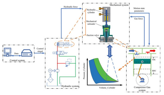
Figure 1.
Stepless capacity control system for a reciprocating compressor.
The valve is the coupling point of the mechanical and gas systems (Figure 2). At different stages, the movement of the valve plate directly affects the thermodynamic parameters, such as the pressure and flow rate of the gas in the cylinder. Tang [5] and Wang [8] observed that valve plate withdrawal is controlled by the unloader, and the decrease in the unloader withdrawal speed directly causes a change in the thermodynamic properties of the gas system, and the upper limit of the unloader is located on the valve plate. Therefore, the ejection and withdrawal speeds of the unloader can be optimized to reduce the impact of the unloader on the gas valve and valve plate on the sealing surface, while ensuring the thermomechanical properties of the gas system.
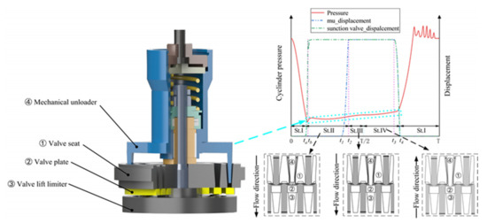
Figure 2.
Coupling relationship between the suction valve and gas system.
The oil inlet pressure and reset spring force are the main power sources and resistance sources for the unloader ejection process, respectively, and the reset spring force and oil return pressure are the main power sources and resistance sources for the unloader withdrawal process, respectively. The matching values of the three parameters determine the unloader motion characteristics.
Therefore, the oil inlet pressure (), oil return pressure (), and reset spring stiffness () were used as optimization variables in this study. The kinematic characteristic parameters of the unloader, i.e., ejection speed () and withdrawal speed (), and the thermodynamic property parameters of the system, i.e., gas work deviation () and flow displacement deviation (), were the optimization objectives. Under different load conditions, the optimum adjustment area of the optimization variable is determined, to achieve the global minimum of the optimization objectives. On the premise of guaranteeing the regulating effect of the flow-regulating system of the compressor, the service life of valves and unloaders is extended, the maintenance cost of the compressor is reduced, and the economic output value of the compressor is increased.
2.2. Model Analysis
2.2.1. Model Establishment
To quantitatively analyze the influence of key parameters on the unloader motion characteristics and the influence on the gas system caused by changes in the unloader and valve motion characteristics, we established a mathematical model of the flow control system, based on multi-system coupling, by considering the unloader dynamic model as the starting point. Furthermore, the coupling relationship between the mechanical, hydraulic, and compressor gas systems was analyzed.
The cylinder gas pressure in the thermodynamic parameters of the reciprocating compressor is the power source for valve opening and closing, and its size affects the movement characteristics of the valve plate. Meanwhile, the effective flow area generated by the valve directly determines the flow rate of the gas, thus changing the compressor displacement and the thermodynamic characteristics of the gas in the cylinder.
The unloader couples the hydraulic cylinder with the valve. The plunger of the hydraulic cylinder pushes the unloader up and down and maintains the ejection state. Consequently, the plunger of the hydraulic cylinder withdraws, and the unloader withdraws under the action of the reset spring.
The mathematical model is built on the following assumptions:
- The rebound during unloader impact is not considered.
- Delays in oil supply or unloading due to the dynamic response of solenoid valves and the pulsation effect of hydraulic lines are not considered, i.e., the starting time of the unloader ejection or withdrawal is the same as that of the oil supply or pressure relief at the hydraulic oil station.
According to the force analysis diagram of the mechanical actuator (Figure 3), during the ejection process, in the time range of (Figure 2), the main power source is hydraulic pressure (Fhy), followed by gravity (Gmu); the main resistance source is reset spring force (FK), followed by suction chamber gas force (Fgs), total friction force (f) and valve disc resultant force (Fv). In the withdrawal process, in the time range (Figure 2), the main power source is the reset spring force (FK), followed by suction chamber gas force (Fgs) and valve disc resultant force (Fv); the resistance source is hydraulic pressure (Fhy), followed by gravity (Gmu) and total friction force (f). The mechanical mechanism is stationary during maintenance, in the time range of . Therefore, the equation for the motion of the actuator is given by Equation (1):
where is the mass of the moving parts of the unloader; xmu is the displacement of the unloader; and is the resultant force on the unloader.
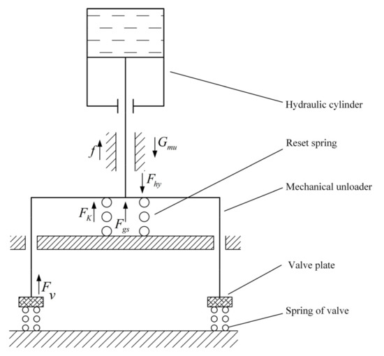
Figure 3.
Diagram of force distribution related to the mechanical actuator.
According to the time-division, we observe that the ejection and withdrawal differential equation of the unloader is given by Equation (2):
where is the force coefficient of interaction between the valve plate and unloader, and is the starting point of the unloader ejection; is the completion of unloader ejection; is the beginning of unloader withdrawal; and is the completion of unloader withdrawal.
The forces in Equation (2) are provided by each subsystem, as follows:
(i) Hydraulic pressure, supplied by the hydraulic system.
The volume chamber at the top of the cylinder plunger constantly interacts with the hydraulic system to create different pressures. According to the node volume cavity method [40], the mathematical model of pressure in the hydraulic cavity is established as follows:
where is the hydraulic pressure of the plunger of the hydraulic cylinder; is the volume elastic modulus of the hydraulic fluid, which is a function of pressure; is the initial pressure of the plunger volume chamber; is the volume of the upper cavity of the piston; and is the hydraulic oil flow.
Because of this assumption, the delay of the pipeline and solenoid valve is not considered in this paper. Based on the incompressibility of oil, the hydraulic pressure depends on the flow of the hydraulic oil and the movement of the external load. The piston in the hydraulic cylinder overcomes the reciprocating motion of friction () and load force () under the action of hydraulic pressure in the chamber. When combined with the pressure established via Equation (3) in the chamber, the equation of motion of the piston is as follows:
where is the flow of hydraulic oil in the hydraulic cylinder; is the cross-sectional area of the plunger of the hydraulic cylinder; is the hydraulic pressure of the plunger of the hydraulic cylinder; is the volume elastic modulus of the hydraulic fluid; is the initial volume of the plunger volume chamber; is the friction of the plunger of the hydraulic cylinder; is the load force of the hydraulic cylinder; and are the masses of the plunger and moving part of the unloader, respectively; and is the displacement of the piston.
The load force of the hydraulic cylinder is the same as that of the unloader: . The movement states of the hydraulic cylinder plunger and unloader are the same: . According to the hydraulic schematic shown in Figure 1, during the ejection process, the hydraulic oil is pumped out of the tank by the hydraulic pump, supplied in one direction to the hydraulic cylinder, and returned to the tank through the one-way intake relief valve. Therefore, the flow rate of hydraulic oil obtained by the hydraulic cylinder comes from the difference between the displacement of the pump and the flow rate of the relief valve. During plunger withdrawal, as the return relief valve is connected in series with the hydraulic circuit (not shown in Figure 1), the outgoing flow of the hydraulic cylinder is mainly dependent on the flow of the return relief valve. According to the principles of hydraulic systems, the flow rate of hydraulic oil in the hydraulic cylinder is related to the pressure settings of the intake and return relief valves. The equation of the flow rate of hydraulic oil in the hydraulic cylinder can be expressed as:
where is the flow of the hydraulic pump; is the flow rate of oil inlet relief valve at inlet pressure setting of ; is the flow of the oil return relief valve at a return pressure setting of ; is the set pressure of the oil inlet overflow valve; and is the set pressure of the oil return overflow valve.
(ii) Return spring force, provided by the mechanical system.
The equation for calculating the return spring force is as follows:
where is the spring stiffness of the unloader; is the spring pre-compression; and is the displacement of the unloader.
(iii) Gas force, supplied by the gas system in the suction chamber of the compressor.
Gas force can be calculated using the following equation:
where is the oil inlet pressure of the suction chamber.
(iv) Valve force, indirectly supplied by the gas system in the compressor cylinder.
As shown in Figure 2, the movement state of the valve plate affects the flow characteristics of the gas, which enters the cylinder from the suction chamber in the suction stage and returns to the suction chamber from the cylinder in the reflux stage. Therefore, the mass flow rate of the gas through the suction valve at different times can be calculated using the following equation [11]:
A reciprocating compressor is a thermodynamic circulating system. According to the first law of thermodynamics, the energy conservation equation of gas in cylinder can be obtained. In order to simplify the calculation, the kinetic energy and potential energy change of gas are ignored. The equation is as follows [41]:
where , , , and represent the heat exchanged between the compressor and the outside world, the enthalpy of the gas sucked in, the enthalpy of the exhaust gas, the energy change of the gas in the compressor cylinder and the output power, respectively.
The gas used in this model is normal-temperature and low-pressure air, and the properties of the gas are close to those of an ideal gas [42]; thus, the gas model is that of an ideal gas [43]:
The thermodynamic parameters in the cylinder vary with changes in the mass flow rate of the gas. By incorporating the gas mass from Equation (8) into the energy conservation equation (Equation (10)), the dynamic pressure in the cylinder is calculated from the following equation at two different stages of suction and reflux:
The movement pattern of the valve plate varies at different stages because of the different forces to which it is subjected. The valve is free before the unloader is ejected, the opening action is completed under the action of the gas force and spring force of the valve, and the plate is maintained and withdrawn at a controlled speed under the force of the unloader during the return and withdrawal stages. The gravity of the valve plate is neglected because it is relatively small compared to other forces. The dynamic analysis of the valve plate at different stages is expressed as follows:
where is the displacement of the valve plate; is the mass of the valve plate; is the force exerted by the actuator; is the gas force acting on the valve plate; and is the valve spring force.
The gas and spring forces acting on the valve plate are calculated from the following equation:
where is the thrust coefficient of the valve plate; is the pressure in the cylinder; is the stress area of the valve plate; Z is the number of valve plate springs; is the rigidity of the valve plate spring; and is the pre-compression of the valve plate spring.
2.2.2. Collaborative Simulation
Based on the operating principle and mathematical model of the flow regulation system, this study has determined the coupling points and interaction parameters of the subsystem of the flow regulation system and established a system-collaborative simulation block diagram according to the analysis results (Figure 4).
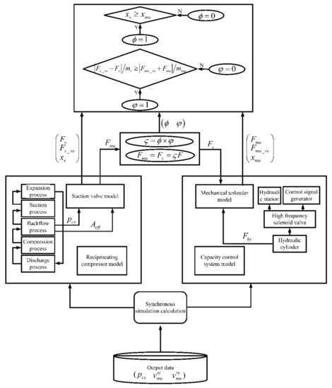
Figure 4.
Co-simulation block diagram of the reciprocating compressor flow control system.
First, the hydraulic system in the flow control system transmits hydraulic pressure to the mechanical system to control the ejection and withdrawal of the unloader. Second, the compressor gas system transmits the gas force to the mechanical system, which affects the movement of the mechanical system; the mechanical system feeds back the displacement parameters to the gas system, which affects the mass flow of the gas system. Third, in the mechanical system, the unloader and valve transmit the interaction force; thus, their motion characteristics affect each other.
The value of the interaction force coefficient () in the mathematical model is determined by the coupling and the mutual interaction between the motion of the unloader and valve plate. This study further established that this is determined by the stress state and the relative position of the unloader and valve plate. In this paper, the relative position and state coefficients are defined; the final interaction coefficient is related to the values of the two coefficients. Since the ejection time of the unloader in this paper occurs after the valve plate is opened, only the coupling between the unloader and valve plate during the withdrawal and maintenance of the unloader is considered. The equations and meanings of the three coefficients are as follows.
The relative position coefficient, , determines whether the unloader and valve plate are in contact with each other, by establishing the position of the unloader and valve plate.
The state coefficient, , under the assumption that the interaction force is not considered, determines whether the speed change of the unloader is less than that of the valve plate.
Regarding the interaction coefficient, , when the relative position and state coefficients are both 1 and they are in contact with each other, the movement of the valve plate is controlled by the movement of the unloader. Therefore, an interaction force between the two is considered to occur at this point in the process.
2.2.3. Model Validation
Based on the joint simulation framework, the stepless flow control system model of the reciprocating compressor was established using the AMESim simulation platform. The key parameters of the DW-12/2 reciprocating compressor test bench were substituted into the above model (Table 1). The experimental and simulation data under different loads were compared according to the average relative error from Equation (14). The results are shown in Figure 5. Under different loads, the full cycle error of the compressor was less than 5%, and the error of different operating processes under different loads was less than 6%, indicating that the fit between the simulation and actual models was high, which provided a simulation basis for the next optimization:
where is the ith data point; is the ith simulated pressure data; is the ith experimental pressure data point; and is the total number of points.

Table 1.
Technical parameters of the experimental compressor.
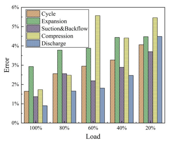
Figure 5.
Model error analysis diagram.
3. Optimization Agent Model and Sensitivity Analysis
3.1. Optimization Agent Model
In this study, the response surface method was used to establish an agent model to simplify the relationship between the key parameterization and objective function. The RSM established the regression response surface model between the objective function and design variables, according to a series of statistical and mathematical methods. The function expression between the objective function and the design variable is expressed as follows:
where w is the approximate function; and is the residual between the true value and the approximate value, which reflects the observation error or noise of the response.
To reflect the nonlinear characteristics between the objective function and design variable, we set the approximate function as a quartic function polynomial. Considering the linear, square, and interaction terms, the quartic polynomial function used in this study can be expressed as follows:
where is the linear effect of ; is the second-order response of ; is the third-order response of ; is the fourth-order response of ; and is the interaction effect of and .
Since the stepless flow regulation system involves different loads, the load factors must be considered synchronously when establishing the agent model. Therefore, the function of the optimized agent model is , where is the load coefficient, with a value of 30–100%.
3.2. Accuracy Analysis of the Agent Model
According to the initial design requirements of the flow control system of the unloader, the value range of the reset spring stiffness was 46,000–80,000 N/m, the value range of the oil inlet pressure was 60–80 bar, and the value range of the oil return pressure was 0–12 bar. According to the practical application of the flow regulation system, when the regulating load was less than 30%, the lubrication effect of the mechanical parts of the compressor decreased, and the gas reflux loss increased, resulting in a decline in the compressor performance. Therefore, 30 samples were obtained using the optimal Latin hypercubic sampling method (Opt-LHD), and the objective function values were calculated under 90–30% load conditions. The agent model was fitted with the experimental data of the design of experiments (DOE) under different loads using the optimization agent model function, and the precision of the agent model was verified by sampling data points randomly. The and of different proxy models in Table 2 indicate that both values were above 0.9, which indicates that the proxy model had high calculation accuracy and could be used satisfactorily.
Table 2.
Calculation accuracy of the optimized agent model.
In this study, the objective was to minimize the residual sum of squares (), optimize the items of the agent model, remove the key items with relatively small influence that had a greater influence on the retention of items, and simplify the agent model while ensuring the accuracy of the agent model. Using an 80% load as an example, the terms and coefficients of the proxy model are listed in Table 3 (The proxy model for the remaining loads is shown in Appendix A). The calculation equation is as follows:
Table 3.
Tables of objective function proxy model parameters at 80% load.
3.3. Sensitivity Analysis
Based on the experimental data of DOE, this study analyzed the influence of design variables on the ejector speed and withdrawal speed of the unloader (Figure 6 and Figure 7). The red line in the diagrams represents the upper limit value of the design variable, and the black line represents the lower limit value of the design variable. If the two lines are not parallel, the response function value is affected by the interaction between the design variables; the higher the degree of parallelism, the stronger the interaction. However, there was no interaction between design variables. In this study, a 90–30% full-load analysis was performed. The 80%, 60%, and 40% loads are selected as examples for illustration.
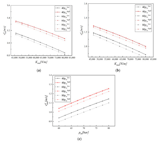
Figure 6.
Effect of design variables on the unloader ejection speed under different loads: (a) Effect of the stiffness of the reset spring and oil inlet pressure on the ejection speed; (b) effect of the stiffness of the reset spring and return pressure on the ejection speed; (c) effect of inlet and return pressures on the ejection speed.
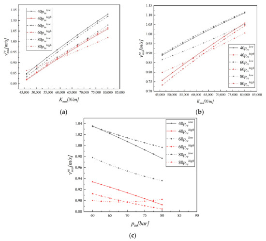
Figure 7.
Effect of design variables on unloader withdrawal speed. (a) Effect of spring stiffness and oil inlet pressure on the withdrawal speed; (b) effect of spring stiffness and oil return pressure on the withdrawal speed; (c) effect of inlet pressure and withdrawal pressure on withdrawal speed.
3.3.1. Ejection Speed
During the ejection process of the unloader, the oil inlet pressure was the main power source, and the rigidity of the reset spring was the main resistance source. As shown in Figure 6a, when the oil inlet pressure was constant, the increase in spring stiffness caused a decrease in the ejection speed. The ejection speed at high inlet pressure was higher than that at low pressure, but the change rate of the ejection speed was almost the same, which indicated that there was no interaction between the spring stiffness and oil inlet pressure. As shown in Figure 6b, when the spring stiffness was constant, the return pressure increased slightly, which resulted in a slight increase in the ejection speed. This was because the inlet flow increased, owing to the increase in return pressure, which indirectly resulted in a slight increase in pressure (Figure 8), but the high and low curves were almost parallel. Therefore, there was no interaction between the spring stiffness and return pressure on the ejection speed. The return pressure was constant, and the increase in inlet pressure caused an increase in ejection speed (Figure 6c), and the two also had no interaction with the ejection speed. Under different loads, the design variables had the same effect on the ejection speed, which meant that the ejection of the unloader was not affected by the load setting.
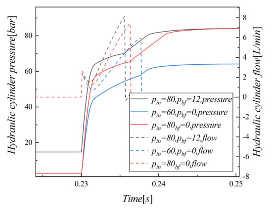
Figure 8.
Inlet flow and pressure of the hydraulic cylinder under different inlet and return pressures.
3.3.2. Withdrawal Speed
During unloader withdrawal, the reset spring was the main power source, and the return pressure was the main resistance source. Figure 7a shows that the withdrawal speed increased with an increase in spring stiffness when the intake pressure was constant, and the withdrawal speed when the intake pressure was high was slower than that at a low intake pressure. This was because the increase in the inlet pressure and the slight decrease in the return flow increased the pressure in the cylinder (Figure 9). Additionally, the change rates of the high and low intake pressures were different, taking into account the spring stiffness, and the two curves were not parallel, which indicated that there was an interaction between the two design variables; the interaction decreased with a decrease in the load. As the main resistance source, the increase in oil return pressure decreased along with the withdrawal speed. As shown in Figure 7b, the withdrawal speed at a high oil return pressure level was lower than that at a low level. Furthermore, with the decrease in load, the interaction effect of the spring’s stiffness and return pressure on withdrawal speed increased, which indicated that the withdrawal speed can be significantly reduced by increasing the backpressure, while decreasing the stiffness of the spring. The increase in return pressure increased the effect of spring stiffness reduction on the withdrawal speed. Figure 7c shows the interaction between the return pressure and inlet pressure, whereby the degree of interaction decreased with a decrease in load.
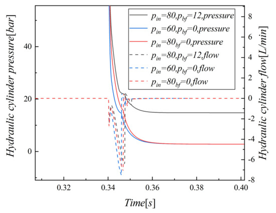
Figure 9.
Return flow and pressure of hydraulic cylinder under different inlet and return pressures.
3.3.3. Deviation in Regulation Performance of the Flow Control System
Valve plate withdrawal was controlled through the unloader withdrawal action. As the withdrawal speed of the unloader decreased, the withdrawal speed of the valve plate decreased continuously, which resulted in an increase in the gas return flow and lagged the compressed discharge process of the compressor, resulting in a deviation in the displacement and regulation performance of the flow control system (Figure 10). Additionally, as the load decreased, the performance of the flow control system deviated further with the decrease in withdrawal speed. Therefore, the deviation in regulation performance under low load should be considered when optimizing the withdrawal speed.
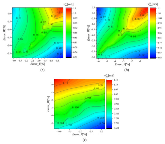
Figure 10.
Relationship between withdrawal speed and control deviation under different loads: (a) 80% load; (b) 60% load; (c) 40% load.
4. Multi-Objective Optimization and Experimental Verification
The multi-objective optimization problem involves determining a set of optimization variables in the applicable area to synchronously minimize a set of contradictory objective functions. In this study, the objective of prolonging the life of the unloader and valve was achieved by reducing the ejection and withdrawal speeds of the unloader. However, from the dynamic equation of the unloader (1), we observed that the power and resistance sources of withdrawal and ejection were opposite, and the objective functions were contradictory. Moreover, owing to the coupling characteristics of the system, the decrease in the withdrawal speed of the unloader and valve plate caused deviations in the flow control and gas power, and there was also a contradiction between the front and back of the setup. Therefore, the problem studied in this paper is a typical multi-objective optimization problem, which is mathematically described as:
where:
is expressed as objective functions; , , and are respectively expressed as flow deviation, gas work deviation, unloader withdrawal speed, unloader ejection speed;
and are inequality constrained functions; is the constraint condition for the unloader to maintain the lower limit; and is the constraint condition for the unloader to maintain the upper limit.
α is the optimized parameter vector; is the stiffness of the reset spring at ; is the intake pressure, ; and is the return pressure, .
For multi-objective optimization, the traditional method transforms the multi-objective problem into a single-objective one by assigning weights to the objectives. However, the second-generation non-dominant sequencing genetic algorithm, NSGA-II, is one of the most effective methods for applying the Pareto optimum concept to multi-objective optimization [44]. The specific procedure of this method can be found in the literature [45]. Based on NSGA-II, this paper proposes a dual optimization method for the optimization of key parameters; it establishes a flow chart of optimization (Figure 11) and combines an ISIGHT-embedded NSGA-II algorithm with AMESim software to optimize the process. First, DOE experiments of the flow regulation system under a full load were performed. Second, an approximate model between the key parameters and objective function was established, which replaced the calculation of the collaborative simulation model. Third, according to the principle of maximum descent ratio and minimum regulation deviation, the optimal design parameters under different loads were obtained through the first and second optimizations. Finally, the optimum design parameters satisfying the full-load optimization were determined according to the simulation experiments, and the actual requirements were determined.
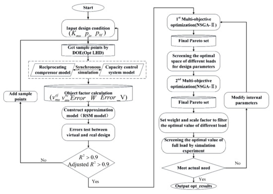
Figure 11.
Process of key parameter optimization.
4.1. Preliminary Selection of Optimization Range
Based on the optimized flow chart and the established optimization agent model, the second-generation non-genetic algorithm, NSGA-II, was selected to optimize the three design variables of inlet pressure, return pressure, and reset spring stiffness, taking the minimum values of the four objective functions, the unloader ejection speed, withdrawal speed, displacement deviation, and work deviation of the flow control system, as objective functions. The initial range of design variables, constraints for adjusting performance deviations, and the parameters of the optimization algorithm are listed in Table 4.
Table 4.
Optimum algorithm for setting parameters.
This study performed the first optimization and key parameter range screening under full-load conditions. The screening process is illustrated using 80%, 60%, and 40% scenarios (Figure 12). According to the optimization criteria, the Pareto front represents all non-inferior solutions after optimization; these are represented by green dots. Owing to the different load approximation models, the shapes of the Pareto fronts were different, and the following conclusions were drawn:
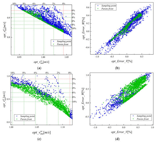
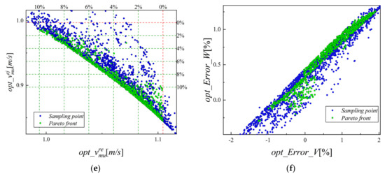
Figure 12.
First optimization result. (a) Optimized speed at 80% load; (b) optimized adjustment deviation at 80% load; (c) optimized speed at 60% load; (d) optimized adjustment deviation at 60% load; (e) optimized speed at 40% load; (f) optimized adjustment deviation at 40% load.
- (1)
- The ejection and withdrawal speeds changed negatively; the ejection speed decreased and the withdrawal speed increased. This was because the power and resistance sources in the two processes were opposite; that is, the ejection power source became the resistance source of withdrawal.
- (2)
- The regulation deviation of the flow control system was positively related, both of which increased and decreased simultaneously, and the value of the load reduction deviation increased. This can be explained by the fact that the lower the load was, the more sensitive the control system was to the change in withdrawal speed, which was consistent with the sensitivity analysis above.
- (3)
- The deviations of regulation performance were within the constraints and were all less than <±5%, which indicated that the optimization results can fully satisfy the system regulation accuracy required by the project.
The objective of optimization was to reduce the unloader ejection and withdrawal speeds and ensure a minimum adjustment deviation. Auxiliary lines with different percentages of speed drop were plotted in the speed diagram, to preliminarily select the optimum range for different loads. The range of the key parameters under different loads was selected according to the maximum reduction ratio of the speed (Table 5). The range data were used as the initial value ranges for the second optimization, to prepare for the final selection.
Table 5.
First optimization results.
4.2. Analysis of Optimized Final Selection Results
According to the principle of maximum reduction ratio, the design variable under 60% load is selected as the initial value of the second optimization, and NSGA-II is used for the second optimization under 30~90% load. By setting the weight and scale factor, the optimal values of the key parameters under different loads are selected with Equation (13), as shown in Table 6. The optimal values obtained under different load conditions are compared by simulation experiments under different loads to find the key parameter setting values that are suitable for full-load condition optimization. Taking the simulation experiment of the optimal values obtained under 40% load, under 80%, 60%, and 40% working conditions, as an example, as shown in Figure 13, the following conclusions are drawn:
Table 6.
Second optimization results.
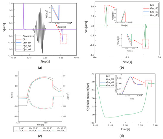
Figure 13.
Simulation results of different optimization design variables at 40% load. (a) Suction valve plate velocity diagram; (b) unload speed diagram; (c) diagram of the unloader resultant force versus valve plate withdrawal acceleration; (d) dynamic pressure diagram of cylinder gas.
- (1)
- Figure 13a,b show the valve plate and unloader speeds, respectively. The unloader of the control system not only reduced the valve plate withdrawal speed but also suppressed the vibration of the valve plate, thus reducing the fatigue damage and impact damage of the valve plate.
- (2)
- The valve plate withdrawal speed decreased with the different optimization parameters. The 60% and 40% loads decreased by almost the same amount and were greater than the 80% load. Similarly, the unloader ejection and withdrawal speeds exhibited the same downward trend.
- (3)
- The change in the movement characteristics of the valve plate caused changes in other flow characteristics, which subsequently changed the thermodynamic parameters of the compressor. As the speed decreased, the system moved into an advanced state; Figure 13d shows that the compression and exhaust processes occurred earlier, resulting in increases in both the adjustment displacement error and work deviation. However, owing to the small proportion of lead time, the deviation was small and the values were less than 5%.
As Figure 13a,b show, the withdrawal endpoints of the discs and unloaders did not lag under the optimized parameters but instead advanced. This was because, during the withdrawal of the unloaders, they were combined by the spring force of the power source and the hydraulic force of the resistance source owing to two points:
- (1)
- Because the stiffness of the reset spring decreased by a small proportion of the optimization parameters, the reset spring force was basically the same as the initial spring force, indicating that the power source was basically the same.
- (2)
- The inlet pressure decreased significantly, resulting in a low initial hydraulic pressure. Additionally, the hydraulic oil outflow speed was slow, owing to the backpressure, which indicated that the initial resistance source was low, and the descent rate was slow. Together, the initial acceleration of the unloader withdrawal under the optimized parameters was large and well-advanced. However, the maximum acceleration was less than the initial parameter acceleration (Figure 13c), which also resulted in a more substantial and earlier start of the unloader withdrawal speed. However, the final speed was less than the initial parameter, and the disc withdrawal was controlled by the unloader for the same reason.
Based on the simulation results, to select the optimum design parameters that can satisfy full-load optimization, the proportion of the unloader ejection and withdrawal speed decreased, and the percentage of decrease in the valve disc withdrawal speed was calculated. As shown in Table 7, the optimization effects of the key parameters obtained under 40% and 30% loads were similar, and the optimized key parameters were almost the same. Therefore, 40% of the optimum value was selected as the optimum design parameter in this study. Compared with the original design value, the stiffness of the reset spring decreased by 6.6%, the inlet pressure decreased by 22.5%, and the return pressure increased by 12 bar:
where is the target variable; is the weight; and is the scale factor.
Table 7.
Simulation results after optimization.
4.3. Verification of Experimental Results
In this study, the design values of key parameters after optimization were verified through full-load condition optimization results, using existing test benches. The results before and after optimization are illustrated using the examples of 80%, 60%, and 40% loads. As shown in Figure 14, the vibration shock loads were 80%, 60%, and 40%, respectively, from top to bottom, the peak value of the ejection vibration shock decreased by 30–40%, and the peak value of the withdrawal shock decreased by 30–50%. Moreover, the impact phase of withdrawal did not deviate significantly, and the end-time of return basically remained unchanged; therefore, the regulation performance of the flow regulating system did not change significantly.
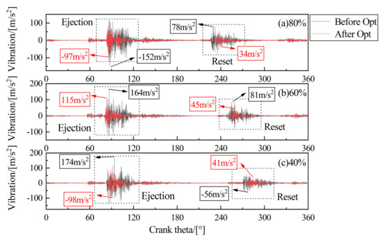
Figure 14.
Comparison of ejection and withdrawal impact of the unloader before and after the optimization of different loads.
To better verify the experimental results, we performed an RMS analysis of the jacking and withdrawing vibration impacts under different loads over a set period. As shown in Figure 15, the effective value of the optimized impact decreased significantly, indicating that the energy generated by the impact decreased significantly, which was conducive to reducing the impact wear of the unloader on the valve plate and of the valve plate on the valve seat.
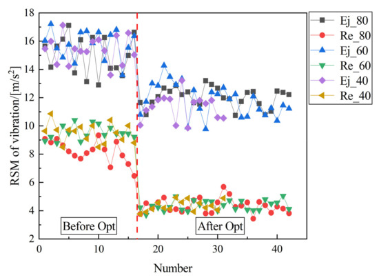
Figure 15.
Comparison of the RMS of ejection and withdrawal shock of the unloader before and after optimization of different loads.
5. Conclusions
This paper presents a detailed analysis of the coupling relationship between the movement characteristics of a mechanical system and the flow characteristics of a gas system and thermodynamic parameters in the flow control system of the reciprocating compressor. Furthermore, the key parameters affecting the unloader action characteristics, including oil inlet pressure, oil return pressure, and reset spring stiffness, are determined, and two evaluation indexes are determined as objective functions, namely, unloader motion characteristics and performance deviation of the flow control system. Based on the airflow control principle of the top-open intake valve, this paper establishes a flow control system simulation model based on multi-system characteristics and compares it with the experimental data to verify the reliability of the model, which can satisfy the requirements of key parameter optimization research. The research results are as follows:
- (1)
- Based on the multi-system simulation model of the flow control system, the DOE test was performed using the optimal Latin hypercubic sampling technology. Based on the test data, we observed no apparent interaction between the three key parameters for the unloader ejection speed, indicating that the three parameters were independent of each other, but for the withdrawal speed, the spring stiffness interacted with the oil inlet and oil return pressures. The degree of interaction between the two differed depending on the load.
- (2)
- The suction valve was the coupling point between the mechanical and gas systems. The change in its motion characteristics directly changed the flow characteristics and thermodynamic properties of the gas in the cylinder. As valve plate withdrawal was controlled by the unloader, the decrease in the unloader withdrawal speed resulted in an increase in the performance bias of the control system, which became more sensitive to the decrease in speed as the load decreased. A low load deviation increased at similar speeds.
- (3)
- Based on the principle of maximum speed decrease ratio and minimum deviation, the optimum values of three key parameters were finally determined, i.e., the intake pressure was 62 bar, the return pressure was 12 bar, and the reset spring stiffness was 74,715 N/m. Via simulation experiments, we observed that relative to the initial design, the maximum reduction ratio of the unloader ejection and withdrawal speeds was more than 5%, the valve plate withdrawal speed decreased to approximately 3%, relative to the free withdrawal of the valve disc, and the reduction ratio of the speed was more than 50%, whereas the performance deviation of the control system was less than <5%.
- (4)
- The experimental results demonstrated that the flow control system operated under the optimized key parameters, the impact energy of the unloader ejection and withdrawal significantly decreased, and the deviation of the regulation performance parameters was small. Therefore, after parameter optimization, the service life of the mechanical system in the flow control system was extended, the overall performance of the system improved, and the energy consumption and cost were reduced.
Author Contributions
Conceptualization, X.S. and Y.W.; methodology, X.S., Y.W., J.Z., F.L., D.Z. and H.H.; software, X.S., Y.W. and J.Z.; validation, X.S. and Y.W.; formal analysis, X.S. and F.L.; investigation, Y.W.; resources, X.S.; data curation, X.S.; writing—original draft preparation, X.S.; writing—review and editing, X.S. and J.Z.; visualization, J.Z.; supervision, J.Z.; project administration, Y.W.; funding acquisition, Y.W. and J.Z. All authors have read and agreed to the published version of the manuscript.
Funding
This work was supported by the National Natural Science Foundation of China (grant number 52101343), the Chongqing Technology Innovation and Application Development Special Project (grant number cstc2020jscx-msxm0411), the Double First-rate Construction Special Funds (grant number ZD1601), the Fundamental Research Funds for the Central Universities (grant number JD2107), and the Fundamental Research Funds for the Central Universities (grant number ZY2016).
Institutional Review Board Statement
This study did not involve humans or animals.
Informed Consent Statement
This study did not involve humans.
Data Availability Statement
The simulated datasets used in this study are available from the corresponding author on reasonable request.
Conflicts of Interest
The authors declare no conflict of interest.
Nomenclature
| area (m2) | |
| flow displacement deviation | |
| gas work deviation | |
| volume elastic modulus of the hydraulic fluid (Pa) | |
| force (N) | |
| gravity (N) | |
| spring stiffness (N/m) | |
| mass (kg) | |
| total number of data points | |
| quantity of heat (J) | |
| gas constant | |
| scale factor. | |
| temperature (°C) | |
| cycle period (s) | |
| average temperature (°C) | |
| proxy function | |
| simplified proxy function | |
| volume (m3) | |
| weight coefficient | |
| target variable | |
| number of valve springs | |
| variable | |
| proxy function coefficient | |
| specific heat capacity at constant volume (J/(kg°C)) | |
| specific heat capacity at constant pressure (J/(kg°C)) | |
| friction (N) | |
| acceleration of gravity (m2/s) | |
| enthalpy unit (J/kg) | |
| adiabatic index | |
| gas mass (kg) | |
| pressure (pa) | |
| flow (m3/s) | |
| time (s) | |
| u | internal energy unit (J/kg) |
| w | approximate function |
| displacement (m) | |
| speed (m/s) | |
| Greek | |
| installation angle of unloader | |
| effective flow area (m2) | |
| interaction coefficient | |
| heat transfer coefficient | |
| coefficient of applied force of gas | |
| relative position coefficient | |
| state coefficient | |
| change quantity | |
| load coefficient | |
| Subscripts | |
| oil return | |
| cylinder | |
| experimental data | |
| effective flow area of air valve | |
| gas chamber | |
| hydraulic piston | |
| hydraulic pressure | |
| the ith data point | |
| oil inlet | |
| the jth data point | |
| cylinder head | |
| load | |
| residual force of mechanical unloader | |
| mechanical unloader | |
| initial value of mechanical unloader | |
| piston | |
| hydraulic oil | |
| pump | |
| cylinder wall | |
| oil inlet relief valve | |
| oil return relief valve | |
| return spring | |
| suction process | |
| simulation data | |
| valve | |
| initial value of valve | |
| stress surface of valve plate | |
| residual force of valve plate | |
| Superscript | |
| ejection process | |
| reset process | |
| optimized value before reset | |
Appendix A
The table of variables and coefficients of the agent model under different loads is supplemented here.
Table A1.
Tables of objective function proxy model parameters at 90% load.
Table A1.
Tables of objective function proxy model parameters at 90% load.
| Object Function | |||||||
|---|---|---|---|---|---|---|---|
| Term | Coefficent | Term | Coefficent | Term | Coefficent | Term | Coefficent |
| −1.93 × 10⁻² | −1.60 × 10⁻³ | −4.61 × 10⁻¹ | 1.25 × 10 | ||||
| −2.50 × 10⁻³ | 1.02 × 10⁻⁶ | −1.25 × 10⁻⁵ | −1.13 × 10⁻⁵ | ||||
| 4.32 × 10⁻⁴ | −9.97 × 10⁻⁴ | 2.66 × 10⁻² | 3.25 × 10⁻² | ||||
| 7.21 × 10⁻⁹ | −1.29 × 10⁻³ | 5.77 × 10⁻⁴ | 5.78 × 10⁻⁵ | ||||
| 2.57 × 10⁻⁸ | −9.04 × 10⁻¹² | 7.88 × 10⁻⁸ | −4.51 × 10⁻³ | ||||
| −7.55 × 10⁻⁵ | 1.06 × 10⁻⁵ | −2.32 × 10⁻⁷ | 3.54 × 10⁻⁸ | ||||
| −6.20 × 10⁻¹⁰ | 8.93 × 10⁻⁹ | −1.30 × 10⁻⁴ | 4.00 × 10⁻⁴ | ||||
| 3.58 × 10⁻⁶ | 1.25 × 10⁻⁸ | −1.41 × 10⁻⁹ | −1.39 × 10⁻⁵ | ||||
Table A2.
Tables of objective function proxy model parameters at 70% load.
Table A2.
Tables of objective function proxy model parameters at 70% load.
| Object Function | |||||||
|---|---|---|---|---|---|---|---|
| Term | Term | Term | Term | Term | Term | Term | Term |
| −1.26 × 10 | −2.78 × 10⁻³ | −5.10 × 10⁻¹ | 7.52 × 10⁻¹ | ||||
| 7.97 × 10⁻⁵ | 1.81 × 10⁻⁶ | −1.30 × 10⁻⁵ | −1.08 × 10⁻⁵ | ||||
| −1.04 × 10⁻³ | −1.80 × 10⁻³ | 2.66 × 10⁻² | 1.50 × 10⁻² | ||||
| −1.87 × 10⁻⁹ | −2.68 × 10⁻³ | 8.74 × 10⁻⁸ | 1.47 × 10⁻² | ||||
| 1.87 × 10⁻⁸ | −1.46 × 10⁻¹¹ | −1.68 × 10⁻⁷ | −5.84 × 10⁻⁵ | ||||
| −3.05 × 10⁻⁵ | 3.95 × 10⁻⁵ | −1.10 × 10⁻⁴ | −5.10 × 10⁻⁴ | ||||
| 1.97 × 10⁻¹⁴ | 1.47 × 10⁻⁸ | −2.11 × 10⁻⁷ | 5.38 × 10⁻⁸ | ||||
| −7.83 × 10⁻²⁰ | 2.25 × 10⁻⁸ | 1.05 × 10⁻⁶ | −1.57 × 10⁻²¹ | ||||
Table A3.
Tables of objective function proxy model parameters at 60% load.
Table A3.
Tables of objective function proxy model parameters at 60% load.
| Object Function | |||||||
|---|---|---|---|---|---|---|---|
| Term | Coefficent | Term | Coefficent | Term | Coefficent | Term | Coefficent |
| 4.19 × 10⁻¹ | −5.25 × 10⁻³ | −7.06 × 10⁻¹ | 7.75 × 10⁻¹ | ||||
| −5.47 × 10⁻⁴ | 1.93 × 10⁻⁶ | 2.26 × 10⁻² | −1.03 × 10⁻⁵ | ||||
| 3.46 × 10⁻⁸ | −1.82 × 10⁻³ | −2.08 × 10⁻¹⁰ | 1.36 × 10⁻² | ||||
| 2.52 × 10⁻⁸ | −2.68 × 10⁻³ | −1.64 × 10⁻⁵ | 1.55 × 10⁻² | ||||
| −3.67 × 10⁻⁵ | −1.56 × 10⁻¹¹ | 6.30 × 10⁻⁸ | −4.48 × 10⁻⁵ | ||||
| 9.54 × 10⁻⁶ | 3.99 × 10⁻⁵ | −2.38 × 10⁻⁷ | −5.59 × 10⁻⁴ | ||||
| −8.75 × 10⁻²² | 1.49 × 10⁻⁸ | 1.27 × 10⁻¹⁵ | 4.94 × 10⁻⁸ | ||||
| −4.86 × 10⁻⁸ | 2.19 × 10⁻⁸ | 1.46 × 10⁻⁶ | −1.70 × 10⁻²¹ | ||||
Table A4.
Tables of objective function proxy model parameters at 50% load.
Table A4.
Tables of objective function proxy model parameters at 50% load.
| Object Function | |||||||
|---|---|---|---|---|---|---|---|
| Term | Coefficent | Term | Coefficent | Term | Coefficent | Term | Coefficent |
| −3.72 × 10⁻¹ | 4.30 × 10⁻³ | −7.96 × 10⁻¹ | 7.57 × 10⁻¹ | ||||
| 2.22 × 10⁻⁵ | 2.38 × 10⁻⁶ | 2.67 × 10⁻² | −1.07 × 10⁻⁵ | ||||
| −4.66 × 10⁻³ | −2.53 × 10⁻³ | −1.36 × 10⁻¹⁰ | 1.45 × 10⁻² | ||||
| −3.28 × 10⁻¹⁰ | −3.18 × 10⁻³ | 5.09 × 10⁻⁸ | 1.55 × 10⁻² | ||||
| 5.01 × 10⁻⁸ | −2.09 × 10⁻¹¹ | −2.17 × 10⁻⁷ | −5.07 × 10⁻⁵ | ||||
| 1.57 × 10⁻⁸ | 5.15 × 10⁻⁵ | −1.06 × 10⁻⁴ | −5.39 × 10⁻⁴ | ||||
| −3.91 × 10⁻⁵ | 2.18 × 10⁻⁸ | 6.75 × 10⁻²¹ | 4.83 × 10⁻⁸ | ||||
| 1.49 × 10⁻¹⁵ | 2.53 × 10⁻⁸ | 1.71 × 10⁻⁶ | −1.37 × 10⁻²¹ | ||||
Table A5.
Tables of objective function proxy model parameters at 40% load.
Table A5.
Tables of objective function proxy model parameters at 40% load.
| Object Function | |||||||
|---|---|---|---|---|---|---|---|
| Term | Coefficent | Term | Coefficent | Term | Coefficent | Term | Coefficent |
| −5.08 × 10⁻² | 3.21 × 10⁻³ | −8.72 × 10⁻¹ | 7.77 × 10⁻¹ | ||||
| 4.89 × 10⁻⁶ | 2.52 × 10⁻⁶ | 2.55 × 10⁻² | −1.06 × 10⁻⁵ | ||||
| −4.30 × 10⁻³ | −2.64 × 10⁻³ | −1.31 × 10⁻³ | 1.40 × 10⁻² | ||||
| −3.90 × 10⁻¹¹ | −3.49 × 10⁻³ | 4.07 × 10⁻⁸ | 1.53 × 10⁻² | ||||
| 6.59 × 10⁻⁴ | −2.07 × 10⁻¹¹ | −2.27 × 10⁻⁷ | −4.53 × 10⁻⁵ | ||||
| 4.08 × 10⁻⁸ | 6.38 × 10⁻⁵ | −2.66 × 10⁻¹⁵ | −5.30 × 10⁻⁴ | ||||
| −9.61 × 10⁻⁵ | 2.16 × 10⁻⁸ | 9.30 × 10⁻⁵ | 4.51 × 10⁻⁸ | ||||
| −2.09 × 10⁻⁶ | 2.64 × 10⁻⁸ | 2.20 × 10⁻²⁰ | −1.24 × 10⁻²¹ | ||||
Table A6.
Tables of objective function proxy model parameters at 30% load.
Table A6.
Tables of objective function proxy model parameters at 30% load.
| Object Function | |||||||
|---|---|---|---|---|---|---|---|
| Term | Coefficent | Term | Coefficent | Term | Coefficent | Term | Coefficent |
| −2.93 × 10⁻¹ | 2.30 × 10⁻² | −8.90 × 10⁻¹ | 9.13 × 10⁻¹ | ||||
| 1.27 × 10⁻⁵ | 3.43 × 10⁻⁶ | 2.51 × 10⁻² | −1.06 × 10⁻⁵ | ||||
| −6.73 × 10⁻³ | −4.10 × 10⁻³ | −1.65 × 10⁻³ | 9.25 × 10⁻³ | ||||
| −1.24 × 10⁻¹⁰ | −5.08 × 10⁻³ | 4.58 × 10⁻⁸ | 1.46 × 10⁻² | ||||
| 1.12 × 10⁻⁷ | −3.06 × 10⁻¹¹ | −1.98 × 10⁻⁷ | −4.76 × 10⁻⁴ | ||||
| 1.31 × 10⁻⁷ | 8.73 × 10⁻⁵ | −2.81 × 10⁻¹⁵ | 5.05 × 10⁻⁸ | ||||
| −1.76 × 10⁻⁴ | 3.51 × 10⁻⁸ | 1.10 × 10⁻⁴ | −1.39 × 10⁻¹⁶ | ||||
| −2.69 × 10⁻⁹ | 3.99 × 10⁻⁸ | 2.32 × 10⁻²⁰ | −1.41 × 10⁻⁹ | ||||
References
- Aprea, C.; Renno, C. Experimental Model of a Variable Capacity Compressor. Int. J. Energy Res. 2009, 33, 23–40. [Google Scholar] [CrossRef]
- Li, D.; Wu, H.; Gao, J. Experimental Study on Stepless Capacity Regulation for Reciprocating Compressor Based on Novel Rotary Control Valve. Int. J. Refrig. 2013, 36, 1701–1715. [Google Scholar] [CrossRef]
- Li, M.L.; Zhao, G.Y.; Hong, W.R.; Chen, B.; Cao, J.L. Valve Plate Roll Analysis on Stepless Capacity Regulation for Reciprocating Compressor. Compress. Technol. 2013, 1, 14–16. (In Chinese) [Google Scholar]
- Pichler, K.; Lughofer, E.; Pichler, M.; Buchegger, T.; Klement, E.P.; Huschenbett, M. Fault Detection in Reciprocating Compressor Valves under Varying Load Conditions. Mech. Syst. Signal Process. 2016, 70–71, 104–119. [Google Scholar] [CrossRef]
- Tang, B.; Zhao, Y.; Li, L.; Wang, L.; Liu, G.; Yang, Q.; Xu, H.; Zhu, F.; Meng, W. Dynamic Characteristics of Suction Valves for Reciprocating Compressor with Stepless Capacity Control System. Proc. Inst. Mech. Eng. Part E J. Process Mech. Eng. 2014, 228, 104–114. [Google Scholar] [CrossRef]
- Hong, W.; Jin, J.; Wu, R.; Zhang, B. Theoretical Analysis and Realization of Stepless Capacity Regulation for Reciprocating Compressors. Proc. Inst. Mech. Eng. Part E J. Process Mech. Eng. 2009, 223, 205–213. [Google Scholar] [CrossRef]
- Jin, J.; Hong, W.; Wu, R. Valve Dynamic Characteristic and Stress Analysis of Reciprocating Compressor Under Stepless Capacity Regulation. J. Fluid Mech. 2009, 415–420. [Google Scholar] [CrossRef]
- Wang, Y.; Zhang, J.; Jiang, Z.; Zhou, C.; Liu, W. Investigation on Thermodynamic State and Valve Dynamics of Reciprocating Compressors with Capacity Regulation System and Parameter Optimization. Eng. Appl. Comput. Fluid Mech. 2019, 13, 923–937. [Google Scholar] [CrossRef]
- Zhang, J.; Zhou, C.; Jiang, Z.; Wang, Y.; Sun, X. Optimization Design of Actuator Parameters with Stepless Capacity Control System Considering the Effect of Backflow Clearance. Appl. Sci. 2020, 10, 2703. [Google Scholar] [CrossRef]
- Liu, G.; Zhao, Y.; Tang, B.; Li, L. Dynamic Performance of Suction Valve in Stepless Capacity Regulation System for Large-Scale Reciprocating Compressor. Appl. Therm. Eng. 2016, 96, 167–177. [Google Scholar] [CrossRef]
- Wang, Y.; Jiang, Z.; Zhang, J.; Zhou, C.; Liu, W. Performance Analysis and Optimization of Reciprocating Compressor with Stepless Capacity Control System under Variable Load Conditions. Int. J. Refrig. 2018, 94, 174–185. [Google Scholar] [CrossRef]
- Zhang, J.; Wang, Y.; Li, X.; Jiang, Z.; Xie, Y.; Zhu, Q. A Simulation Study on the Transient Motion of a Reciprocating Compressor Suction Valve Under Complicated Conditions. J. Fail. Anal. Prev. 2016, 16, 790–802. [Google Scholar] [CrossRef]
- Xiuqing, Y.; Minzhou, L.; Tao, M.; Damao, Y. Co-Simulation Research of the Mechanical-Hydraulic-Control Coupling System of ITER Tractor. Plasma Sci. Technol. 2009, 11, 334–340. [Google Scholar] [CrossRef]
- Ma, J.G.; Wu, Z.Z.; Guo, H.R.; Li, J. Design and Simulation Study of a Certain Landing Gear Loading Simulation System. Adv. Mat. Res. 2014, 871, 69–76. [Google Scholar] [CrossRef]
- Trikande, M.W.; Jagirdar, V.V.; Rajamohan, V.; Sampat Rao, P.R. Investigation on Semi-Active Suspension System for Multi-Axle Armoured Vehicle Using Co-Simulation. Def. Sci. J. 2017, 67, 269–275. [Google Scholar] [CrossRef][Green Version]
- Zeng, Q.; Gao, K.; Zhang, H.; Jiang, S.; Jiang, K. Vibration Analysis of Shearer Cutting System Using Mechanical Hydraulic Collaboration Simulation. Proc. Inst. Mech. Eng. Part K J. Multi Body Dyn. 2017, 231, 708–725. [Google Scholar] [CrossRef]
- Spiryagin, M.; Simson, S.; Cole, C.; Persson, I. Co-Simulation of a Mechatronic System Using Gensys and Simulink. Veh. Syst. Dyn. 2012, 50, 495–507. [Google Scholar] [CrossRef]
- Zhou, L.; Yan, G.; Ou, J. Response Surface Method Based on Radial Basis Functions for Modeling Large-Scale Structures in Model Updating. Comput. Aided Civ. Infrastruct. Eng. 2013, 28, 210–226. [Google Scholar] [CrossRef]
- Ezhilsabareesh, K.; Rhee, S.H.; Samad, A. Shape Optimization of a Bidirectional Impulse Turbine via Surrogate Models. Eng. Appl. Comput. Fluid Mech. 2018, 12, 1–12. [Google Scholar] [CrossRef]
- Han, H.; Yu, R.; Li, B.; Zhang, Y.; Wang, W.; Chen, X. Multi-Objective Optimization of Corrugated Tube with Loose-Fit Twisted Tape Using RSM and NSGA-II. Int. J. Heat Mass Transf. 2019, 131, 781–794. [Google Scholar] [CrossRef]
- He, Q.; Ma, D.; Zhang, Z.; Yao, L. Mean Compressive Stress Constitutive Equation and Crashworthiness Optimization Design of Three Novel Honeycombs under Axial Compression. Int. J. Mech. Sci. 2015, 99, 274–287. [Google Scholar] [CrossRef]
- Yaghoobi, H.; Taheri, F. Analytical Solution and Statistical Analysis of Buckling Capacity of Sandwich Plates with Uniform and Non-Uniform Porous Core Reinforced with Graphene Nanoplatelets. Compos. Struct. 2020, 252, 112700. [Google Scholar] [CrossRef]
- Song, T.; Yao, Y.; Ni, L. Response Surface Method to Study the Effect of Conical Surface and Vortex-Finder Lengths on de-Foulant Hydrocyclone with Reflux Ejector. Sep. Purif. Technol. 2020, 253, 117511. [Google Scholar] [CrossRef]
- Chiandussi, G.; Codegone, M.; Ferrero, S.; Varesio, F.E. Comparison of multi-objective optimization methodologies for engineering applications. Comput. Math. Appl. 2012, 63, 912–942. [Google Scholar] [CrossRef]
- Li, H.; Zhang, Q. Multiobjective Optimization Problems with Complicated Pareto Sets, MOEA/D and NSGA-II. IEEE Trans. Evol. Comput. 2009, 13, 284–302. [Google Scholar] [CrossRef]
- Mostaghim, S.; Teich, J. Strategies for Finding Good Local Guides in Multi-Objective Particle Swarm Optimization (MOPSO). IEEE Lat. Am. Trans. 2003, 2, 26–33. [Google Scholar] [CrossRef]
- Yang, X.S.; Karamanoglu, M.; He, X. Flower Pollination Algorithm: A Novel Approach for Multiobjective Optimization. Eng. Optim. 2014, 46, 1222–1237. [Google Scholar] [CrossRef]
- Mirjalili, S.; Saremi, S.; Mirjalili, S.M.; Coelho, L.D.S. Multi-Objective Grey Wolf Optimizer: A Novel Algorithm for Multi-Criterion Optimization. Expert Syst. Appl. 2016, 47, 106–119. [Google Scholar] [CrossRef]
- Wu, K.A.; Yan, X.H.; Chen, Z.X. Hybrid multi-objective evolutionary algorithm based on Pareto sort. Comput. Eng. Appl. 2015, 51, 62–68. (In Chinese) [Google Scholar]
- Yang, Y.; Liu, J.; Tan, S.; Wang, H. Application of Constrained Multi-Objective Evolutionary Algorithm in Multi-Source Compressed-Air Pipeline Optimization Problems. IFAC-PapersOnLine 2018, 51, 168–173. [Google Scholar] [CrossRef]
- Zhang, L.; Chen, L.; Xia, S.; Ge, Y.; Wang, C.; Feng, H. Multi-Objective Optimization for Helium-Heated Reverse Water Gas Shift Reactor by Using NSGA-II. Int. J. Heat Mass Transf. 2020, 148, 119025. [Google Scholar] [CrossRef]
- Demissie, A.; Zhu, W.; Belachew, C.T. A multi-objective optimization model for gas pipeline operations. Comput. Chem. Eng. 2017, 100, 94–103. [Google Scholar] [CrossRef]
- Jiang, J.; Cai, H.; Ma, C.; Qian, Z.; Chen, K.; Wu, P. A Ship Propeller Design Methodology of Multi-Objective Optimization Considering Fluid–Structure Interaction. Eng. Appl. Comput. Fluid Mech. 2018, 12, 28–40. [Google Scholar] [CrossRef]
- Horn, J.; Nafpliotis, N.; Goldberg, D.E. A niched Pareto genetic algorithm for multiobjective optimization. Proceedings of the First IEEE Conference on Evolutionary Computation. IEEE World Congr. Comput. Intell. 1994, 82–87. [Google Scholar] [CrossRef]
- Zitzler, E.; Thiele, L. Multiobjective evolutionary algorithms: A comparative case study and the strength Pareto approach. IEEE Trans. Evol. Comput. 1999, 3, 257–271. [Google Scholar] [CrossRef]
- Shu, Y.; Yong, S.; Chang, Q. Performance Assessment and Optimal Design of Hybrid Material Bumper for Pedestrian Lower Extremity Protection. Int. J. Mech. Sci. 2020, 165, 105210. [Google Scholar] [CrossRef]
- Cui, Y.; Geng, Z.; Zhu, Q.; Han, Y. Review: Multi-objective optimization methods and application in energy saving. Energy 2017, 125, 681–704. [Google Scholar] [CrossRef]
- Liu, C.B.; Bu, W.Y.; Dong, X. Multi-objective shape optimization of a plate-fin heat exchanger using cfd and multi-objective genetic algorithm. Int. J. Heat Mass Transf. 2017, 111, 65–82. [Google Scholar] [CrossRef]
- Jiang, Z.N.; Zhou, C.; Wang, Y.; Zhang, J.J.; Sun, X. Optimization design of actuator parameters in multistage reciprocating compressor stepless capacity control system based on NSGA-II. Math. Probl. Eng. 2020, 2020, 7581845. [Google Scholar] [CrossRef]
- Gao, Q.H.; Wang, S.A.; Huang, X.F. Model Library Build for Hydraulic System Simulation with SIMULINK. Syst. Simul. Technol. Appl. 2006, 8, 317–320. (In Chinese) [Google Scholar]
- Armaghani, T.; Sahebi, S.; Goodarzian, H. The first law simulation and second law analysis of a typical reciprocating air compressor. Indian J. Sci. Technol. 2012, 5, 2390–2395. [Google Scholar] [CrossRef]
- Mamedov, B.A.; Somuncu, E.; Askerov, I.M. Theoretical Assessment of Compressibility Factor of Gases by Using Second Virial Coefficient, Zeitschrift Fur Naturforsch. Sect. A J. Phys. Sci. 2018, 73, 121–125. [Google Scholar] [CrossRef]
- Jin, J.M.; Hong, W.R. Valve dynamic and thermal cycle model in stepless capacity regulation for reciprocating compressor. Chin. J. Mech. Eng. 2012, 25, 1151–1160. [Google Scholar] [CrossRef]
- Srinivas, N.; Deb, K. Muiltiobjective Optimization Using Nondominated Sorting in Genetic Algorithms. Evol. Comput. 1994, 2, 221–248. [Google Scholar] [CrossRef]
- Deb, K.; Pratap, A.; Agarwal, S.; Meyarivan, T. A fast and elitist multiobjective genetic algorithm: NSGA-II. IEEE Trans. Evol. Comput. 2002, 6, 182–197. [Google Scholar] [CrossRef]


Publisher’s Note: MDPI stays neutral with regard to jurisdictional claims in published maps and institutional affiliations. |
© 2022 by the authors. Licensee MDPI, Basel, Switzerland. This article is an open access article distributed under the terms and conditions of the Creative Commons Attribution (CC BY) license (https://creativecommons.org/licenses/by/4.0/).