Article

A Numerical Study on Blade Design and Optimization of a Helium Expander for a Hydrogen Liquefaction Plant

1
Department of Energy Conversion Systems, Korea Institute of Machinery & Materials, Daejeon 34103, Korea
2
Department of System Dynamics, Korea Institute of Machinery & Materials, Daejeon 34103, Korea
3
Innovatium, Glasgow G46 8NG, Scotland, UK
*
Author to whom correspondence should be addressed.
Appl. Sci. 2022, 12(3), 1411; https://doi.org/10.3390/app12031411
Submission received: 8 January 2022 / Revised: 25 January 2022 / Accepted: 25 January 2022 / Published: 28 January 2022
(This article belongs to the Section Mechanical Engineering)

Abstract

:
A design process for cryogenic expanders that supplies 0.5 TPD of liquefied hydrogen in hydrogen liquefaction plants is introduced. To improve the efficiency of the expander, the optimum design was conducted by adjusting two rotor shape parameters. The designed expander for hydrogen liquefaction has a target rotation speed of 75,000 rpm, and helium is applied as the working fluid. Since the operating temperature of the expander is as low as 49 K, a design that reflects the real gas properties must be considered. For a high-efficiency hydrogen liquefaction plant, increasing the expander efficiency is one of the most critical issues. In this study, the efficiency of the cryogenic expander was optimized using the response surface method (RSM). The hub and shroud meridional contours and blade β angle distributions were chosen as the design parameters. As a result, through the optimized design, it was possible to improve the expander efficiency by up to 1.98% compared to the original expander. Flow analysis was conducted to investigate the reason for the efficiency improvement. Through this study, the effect of the blade meridional contour and blade β angle on the cryogenic expander efficiency was verified.

1. Introduction

A new climate regime, POST-2020, was agreed upon at the climate change conference held in Paris in December 2015. In order to implement this new climate system, all countries must strive to achieve their greenhouse gas reduction targets. To this end, many efforts are being made to develop clean energy worldwide. Representatively, there have been studies on the production and use of hydrogen energy. Recently, a full-scale study on the development of core technologies for hydrogen liquefaction plants began in South Korea.
A hydrogen liquefaction plant is a closed-loop system, and it consists of a compressor, heat exchanger, cold box, and expander. The expander is one of the core components in a cryogenic system. In the cryogenic expander, the working fluid is expanded under extremely low temperatures, e.g., below 93 K. Therefore, some of the parts, i.e., the rotor, shaft, and labyrinth seal, are operated under cryogenic conditions. In general, the cryogenic expander rotates at a high speed, from tens of thousands to hundreds of thousands of revolutions per minute, so rotordynamic stability is important.
The technologies required to develop the cryogenic expander are as follows: aerodynamic design technology with an expander loss model for cryogenic working fluids, seal and insulation technology, thermal stress analysis technology, high-speed oil-free bearing technology, clearance prediction and control technology, secondary flow stabilization technology, and expander power control technology. However, because of the information security of the industry, the introduction of these technologies in the literature or at conferences has been limited. However, it is possible to identify the latest technology trends and technical issues through the publications of a few companies that produce cryogenic expanders [1,2,3].
There are several methods to exhaust the output power generated by the expander. First, a compressor is installed on the opposite side of the expander with the same shaft. It can be applied to compress the working fluid at the cryogenic system [4]. This expander–compressor assembly is called a compander. When it is used as a compander, there is an advantage in that the high pressure required in the cryogenic system can be acquired from the compressor. However, there is a disadvantage in that the system operation is complicated.
Second, the power generated from the expander drives the brake compressor to exhaust energy [5,6,7,8]. Alternatively, there is a method of converting the power generated by the expander into heat energy using an eddy current breaker. It has an advantage in that the size of the system can be reduced and the control can be made simple. However, it dissipates the energy generated by the expander; therefore, it is not preferable for a large-capacity plant. Third, the expander rotates the generator, and electric power can be acquired from the generator. If the capacity of the expander is large enough, the application of a generator can be considered.
As described above, the method of utilizing expander energy can be determined by the characteristics of the cryogenic system. In this research, the brake compressor is connected to the expander so that the speed of the expander can be controlled by adjusting the compressor’s throttle valve.
Song et al. conducted blade optimization to reduce the swirl flow and cavitation in the draft tube of a cryogenic liquid turbine [9]. Huang et al. investigated the effect of the blade loading distribution and blade lean angles on the cavitation in the draft tube of a cryogenic expander [10]. However, there has been little research on the optimization of cryogenic expander efficiency.
To develop a highly efficient cryogenic system, it is necessary to increase the efficiency of the expander. In this paper, the optimization of an expander rotor was conducted to improve expander efficiency. The expander rotor rotates at tens of thousands of revolutions per minute under cryogenic conditions. However, there is no sufficient design modeling for an expander with cryogenic fluids. Therefore, careful decisions must be made on the shape factors that determine the efficiency of the expander.
In this study, the rotor blade meridional shape and blade β angle were optimized to improve the expander efficiency. This can be used as a reference to design a high-efficiency cryogenic expander in the future.

2. Operation Conditions

In this study, cycle analysis was conducted to develop a high-efficiency hydrogen liquefaction system. Through the cycle analysis, the operating conditions of the component were determined. The target capacity of the hydrogen liquefaction system is condensing 0.5 tons of hydrogen per day. Figure 1a shows a schematic of a 0.5-TPD class hydrogen liquefaction plant. The helium working fluid absorbs the cold heat of the vaporized nitrogen through a heat exchanger (Hx1), and by flowing through a sequence of heat exchangers and expanders, the temperature is lowered so that hydrogen can be liquefied. Hydrogen in the gaseous state is liquefied through heat exchangers Hx1−Hx4 and stored in a tank.
As shown in Figure 1a, the system consists of two expanders, one compressor, and four heat exchangers. The expanders are connected in series. In this study, design and optimization were conducted for one of the expanders.
Figure 1b illustrates the temperature–entropy (T–s) diagram of the hydrogen liquefaction plant. Table 1 shows the components in each process in the T–s diagram. A heat exchanger (process ④–⑤ in Figure 1) is installed between Expander 1 and Expander 2. The expander that was studied in this research was Expander 1, which relates to processes ③–④ in the system.
Table 2 presents the operation conditions of the expanders. The considered expansion ratios of Expander 1 and Expander 2 were 1.6 and 3.69, respectively.

3. Expander Design

3.1. Preliminary Design

A preliminary design was performed to determine the rotational speed and diameter of the expander rotor. In the preliminary design, specific velocity and specific diameter analyses were conducted. The definitions of the specific velocity and specific diameter are as follows:
Specific   speed :   N s = ω Q 6 h i s e n 0.75  
Specific   diameter :   D s = d h i s e n 0.25 Q 6  
Table 3 shows the preliminary design results for Expander 1.
In the case of a centrifugal expander, the specific speed is generally selected between 0.5 and 0.6 in consideration of expander efficiency. However, in this study, the specific speed of the expander was selected as 0.392, considering rotordynamic performance. The design speed was 75,000 rpm. Through specific diameter analysis, it was estimated that the diameter of the rotor should be 53.77 mm.
In the case of the radial inflow expander, the relation of the specific speed N s and the specific diameter D s was N s × D s = 2 [11]. Therefore, the specific diameter D s was determined when the specific velocity N s was chosen. For this reason, U_tip in Table 3 is the same against the specific velocity N s .

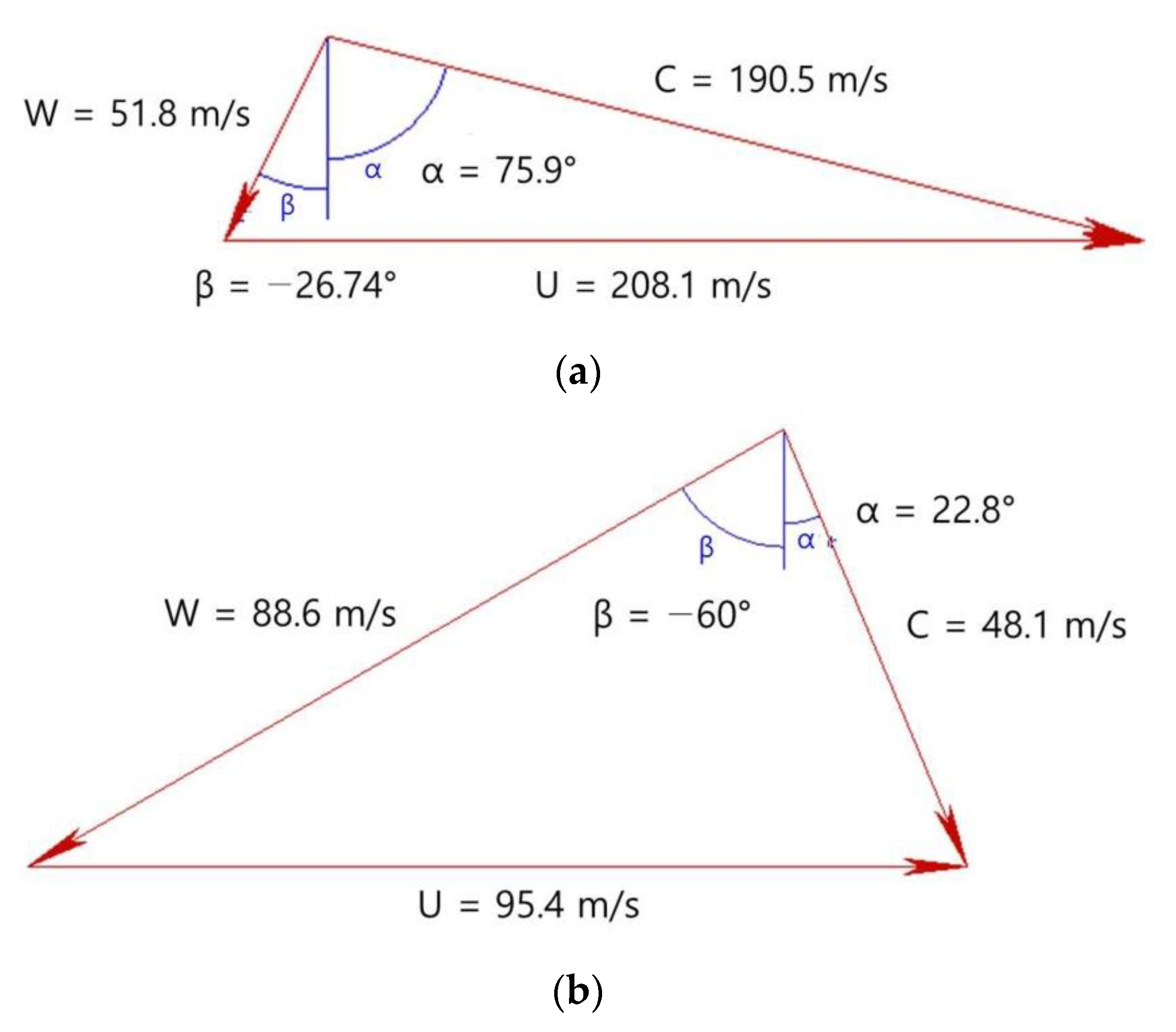
3.2. Meanline Design

Meanline design, which is also called one-dimensional design, was conducted based on the results of the preliminary design. Meanline design is a flow path design including the blade shape and flow angle. In this study, meanline design was conducted using ConceptsNREC Inc’s RITAL program. The Rodgers loss model was applied for the nozzle design, and the CETI passage loss model was applied for the rotor design.
Figure 2 shows the meanline shape of the expander. The designed expander consists of a volute, nozzle, and rotor. Generally, a volute is symmetric. However, in this research, an overhang-shaped volute was selected to shorten the shaft length and increase the assembly. Cho et al. compared losses according to the shape of volute [12]. They conducted a CFD analysis of the loss in a circular volute and a rounded square volute. In this study, the volute shape was determined based on the fact that a circular volute has less loss than that of a rounded square volute. The major dimensions of the expander are shown in Table 4. The designed tip clearance between the rotor and shroud was 0.3 mm.
The velocity triangles at the inlet and outlet of the rotor are shown in Figure 3. In this study, the incidence angle was −26.74°, and the deviation angle was 22.8°. Figure 4 shows the performance curves derived from the meanline design. They were plotted at 80% (60,000 rpm), 90% (67,500 rpm), and 100% (75,000 rpm) of the design speed.
Figure 4a shows the relation between the expansion ratio and mass flow rate. Figure 4b shows the relation between the expansion ratio and efficiency. The efficiency from the meanline design was recalculated by reflecting the loss in the expander. It is defined as the ratio of the enthalpy difference and isentropic enthalpy difference between the inlet and outlet of the expander. It was verified that the target efficiency was satisfied at the design expansion ratio. Figure 4c shows the relation between the expansion ratio and the power. Like the efficiency curve, the power from the meanline design was recalculated by reflecting the loss in the expander. Finally, Figure 4d shows the relation between the expansion ratio and the expander outlet temperature. The cryogenic expander must satisfy the expander outlet temperature in the system requirements. As shown in the figure, the estimated expander outlet temperature meets the design temperature.

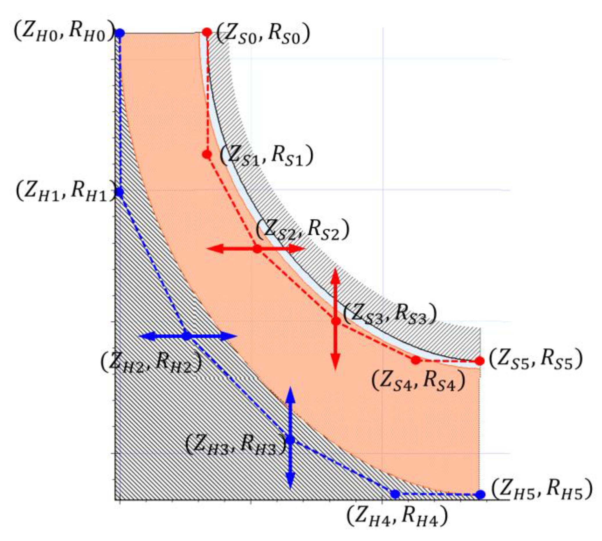
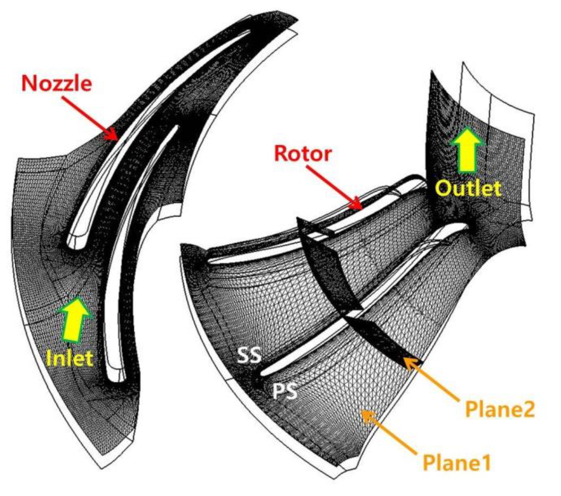
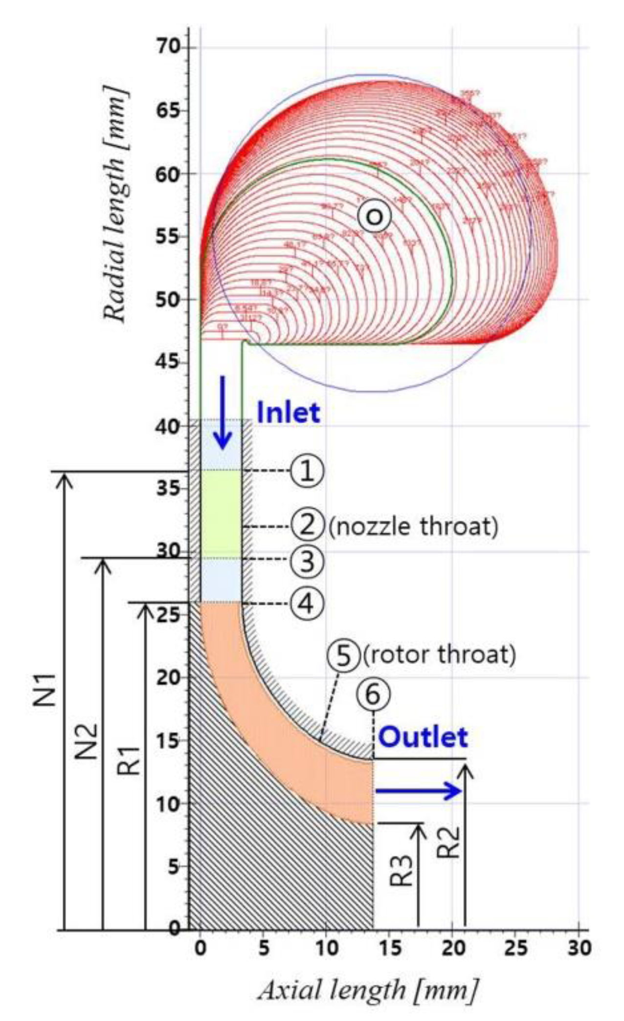
3.3. 3D Shape Generation

Based on the results of the meanline design, a three-dimensional expander geometry was generated to conduct the numerical analysis. The three-dimensional geometry was generated using AxCent program of ConceptsNREC. Figure 5 shows the 3D shapes of the nozzle and rotor.
Considering the assembly of the expander, the length of the straight zones between the volute and nozzle inlet and between the nozzle and the rotor were determined. The trailing edge thickness was determined considering the blade manufacturer. The shape of the leading edge was rounded to prevent separation at the leading edge of the rotor.

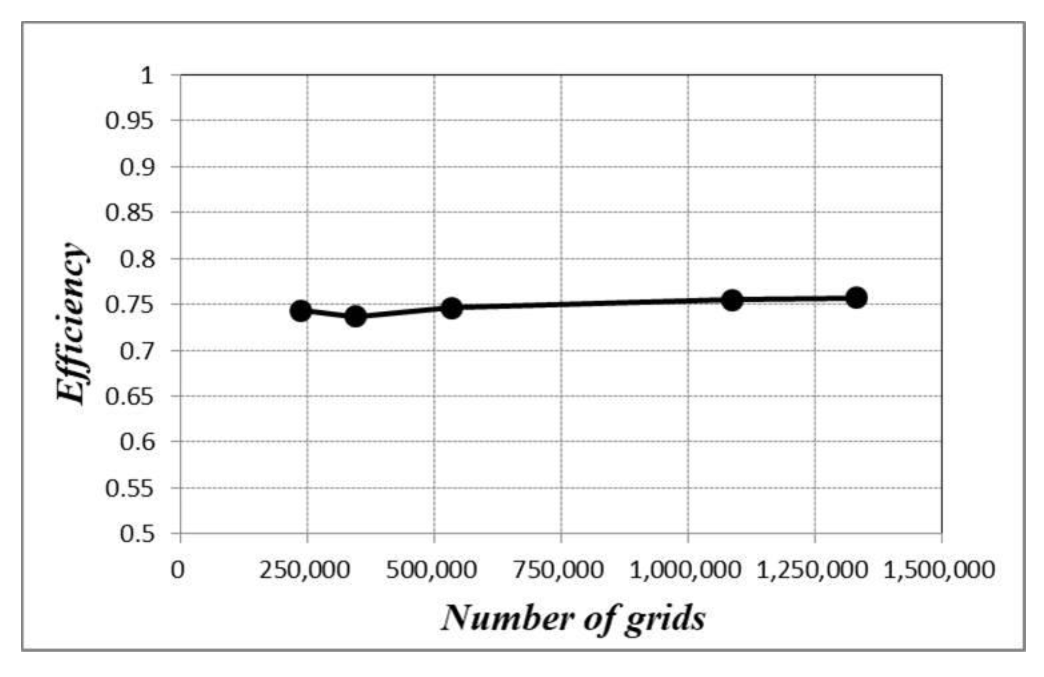
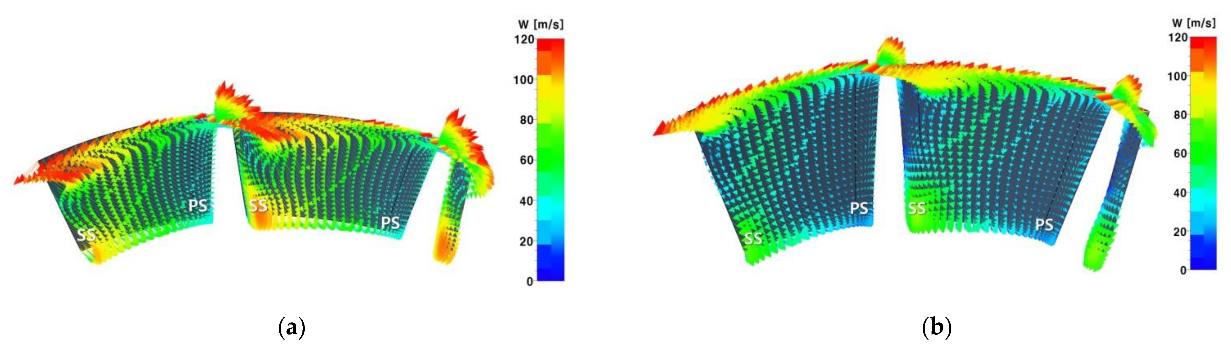
3.4. Numerical Analysis

Numerical analysis was conducted using NUMECA’s FINE/Turbo program. As a turbulence model, the Spalart–Allmaras model, a one-equation model with excellent calculation efficiency, was applied to determine the exact properties of the boundary layer in the pressure gradient.
In order to increase the convergence of the calculation, the choice of boundary condition is important. In general, pressure, temperature, and flow rate are applied as boundary conditions in turbomachinery numerical analysis. Applicable pressure and temperature values are static and stagnation value. In addition, the applicable flow information is the mass flow rate and the velocity vector. In this study, numerical analysis was performed by analyzing the calculated result using the pressure condition as the main boundary condition. The applied boundary conditions were the inlet total pressure, inlet total temperature, velocity direction, turbulent viscosity, and outlet static pressure. To obtain the off-design point performance, the outlet static pressure was varied. The meanline design results were used for the flow angle information flowing into the nozzle inlet. That is, the absolute flow angle of the volute outlet was used as the nozzle inlet flow angle in the numerical analysis.
A mixing plane condition was applied between the nozzle outlet and the rotor inlet. Therefore, the average physical property value in the pitch direction was applied as the rotor inlet condition. In real operation conditions, the shape of the nozzle wake changes along with the rotor revolution, and to analyze it, unsteady calculations should be conducted. In this study, the focus was on efficiency improvement, and a steady calculation was conducted. The calculation was conducted for a single periodic passage.
To determine the appropriate number of grids, the efficiency according to the number of grids was analyzed. Efficiency was compared for the following number of grids: 199,079, 239,403, 345,415, 534,415, 1,088,147, and 1,332,851. When the number of grids was greater than 239,403, there was no significant change in efficiency. In this study, the number of grid cells in the calculation domain was 1,088,147. Figure 6 shows the relationship of efficiency according to grid number to check grid independence. A hexa mesh was applied to generate a dense grid near the blade wall, and Y+ was set to 2.
The cryogenic expander design was conducted using the real gas properties of helium. To reduce the computation time during the numerical analysis, a property table of the working fluid was applied to the calculation. NUMECA’s TabGen was used to generate the data. TabGen creates a fluid property table in connection with NIST’s REFPROP, a program that provides fluid properties. Interpolation was performed based on the generated property table so that it could be used as a property value at a location necessary for numerical analysis.
Figure 7 shows the performance curves of the cryogenic expander derived from the numerical analysis. In the same way as for the meanline design results, the mass flow rate, efficiency, power, and outlet temperature were plotted against the expansion ratio at 80%, 90%, and 100% of the design speed. The efficiency and power from the numerical analysis were recalculated by taking into account the extra mechanical losses in the expander. The extra mechanical losses were the loss caused by the volute and the loss caused by the windage in the rotor back disk, and in this study, the losses were assumed to be 2% and 4%, respectively. The outlet temperature of the expander satisfies the temperature required by the system.

4. Optimization

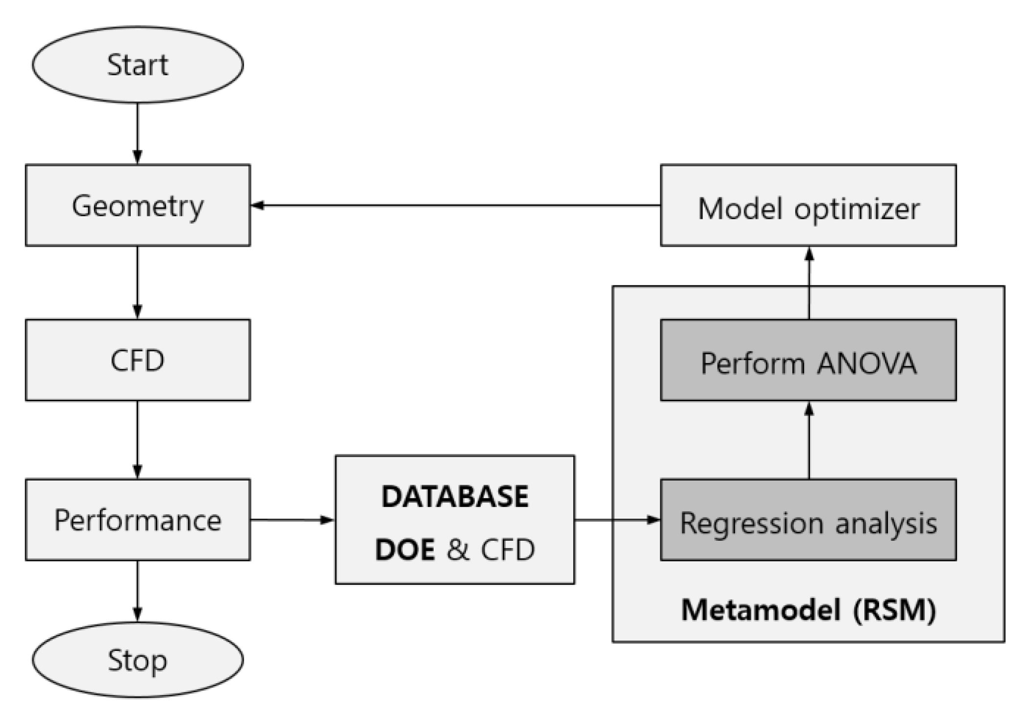
4.1. Optimization Methodology

Optimization is an effective tool for selecting the best design among a variety of available options through identifying design variables and design objectives. Figure 8 shows a schematic of the design optimization process in this study. The initial design geometry was obtained via meanline design, and the performance of the design geometry was evaluated via CFD. The building of a database using design of experiments (DOE) and obtaining and optimizing a metamodel were performed using Minitab software. Metamodel optimization allows special insight into system performance and allows the system to be examined across a wide range of design conditions at a relatively modest computational cost [13].
Optimization starts with building a database using DOE. The number of regression model coefficients increases rapidly as the number of design parameters increases. Various DOEs have been proposed to obtain a highly accurate response surface function with a minimum number of experiments under given conditions. In this study, the Box–Behnken design method was adopted because it can derive quadratic regression equations, easily create orthogonal blocks, and use fewer design points than 3k-factorial design or central composite design [14]. The boundaries of the design space were normalized to the range selected for each design parameter so that the existing geometry value was set to 0 and the maximum range of change for the design variables was set to ±1. For 4 design variables, 25 test cases were designed to obtain the equation relating the design parameters and the objective function. In each test case, two design variables were fixed at 0, the existing geometry value, and the other two variables were set to ±1.
A meta-model was built using the DOE points to construct the function F correlating the objective functions U j with the design parameters X i as follows:
U j = F j ( X i )                           i = 1 ,     N               j = 1 ,               M
In the present study, the response surface method (RSM) was used to obtain an optimal design. It is widely used among approximate model-based design optimization techniques. The RSM is a technique that approximates the response surface function from the value of the objective function obtained after performing 3D CFD on a set of design variables. The response surface function U j can be expressed as a quadratic polynomial using the design parameters X i and X j as follows:
U j = β O j + i = 1 n β i j X i + i = 1 n β i i j X i 2 + i < k n β i k j X i X k  
where β O , β i , β i i , and β i k are the polynomial coefficients, and these undefined coefficients are determined via least square regression using the 3D CFD results. A detailed analysis of the effect of parameters and their interactions on the response was also performed through the surface plots using Minitab software. In the response surface method, the reliability of the response surface function can be checked, and this reliability can be increased by removing insignificant undefined coefficients, which is called response surface model pooling. Response surface model reduction is achieved through analysis of variance (ANOVA) and regression analysis. The analysis of variance is used to determine whether each term of the response surface function is significant, and the significance is confirmed under the condition that the significance probability p is <0.05. Insignificant terms are removed in the order of block, alternating term, and square term, and analysis of variance is performed. After the analysis of variance is finished, regression analysis is performed. Regression analysis is an analysis method that measures the fitness of how well the response surface function represents the actual value, and it is determined by the R2adj (correction coefficient of determination) of the response surface function. That is, if R2adj > 0.9, the response surface function is very accurate, and if 0.9 > R2adj > 0.7, the response surface function is relatively accurate [15,16].
An optimal point of the response surface provides a new design geometry. The performance of the optimal design geometry is then evaluated. This optimization process repeats until the objective function reaches the target value.

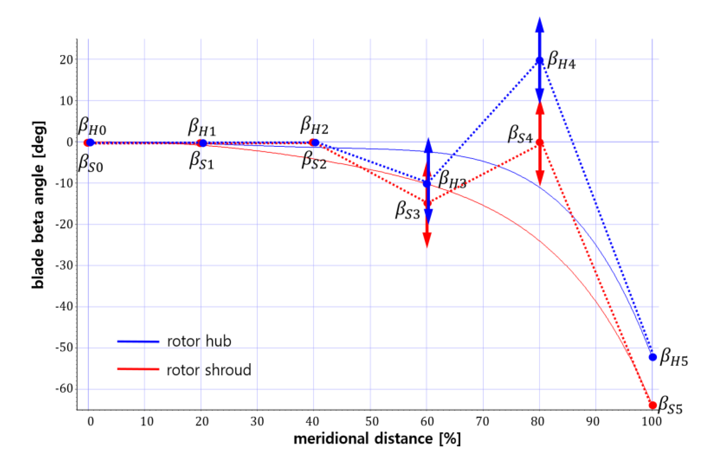
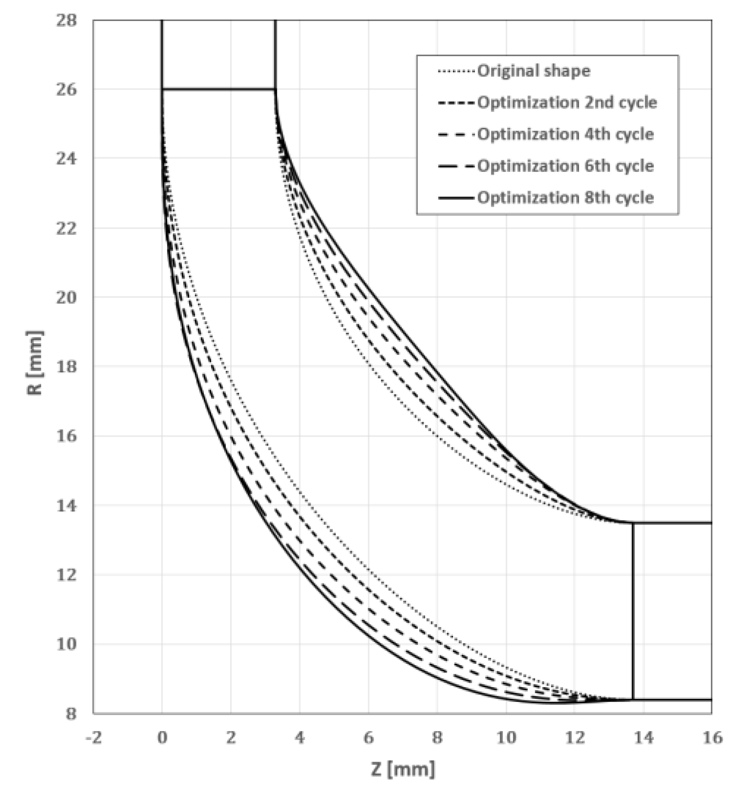
4.2. Optimization of the Expander

Since the aim of the optimization in the present work is to maximize the total-to-total efficiency for the given design specification, the isentropic total-to-total efficiency of the expander at the design point was considered the objective function, as Equation (5) shows:
η T T = h T 0 h T 6 h T 0 h T 6 i s e n
where h T 0 is the expander inlet total enthalpy, h T 6 is the expander outlet total enthalpy, and h T 6 i s e n is the expander outlet total enthalpy in isentropic conditions of the expander inlet.
The hub and shroud meridional contours in the z–r plane and the blade β angle distributions at the hub and shroud were chosen as the design parameters of the 3D radial expander rotor. The hub and shroud meridional contours and the control points of each Bezier curve are shown in Figure 9. The locations of the inlet and outlet points were fixed. To maximize the shape profiles with the minimum number of test cases, and Z H 2 , R H 3 , Z S 2 , and R S 3 were selected as the design parameters for the optimization of the meridional contours. Figure 10 shows the blade β angle distributions at the hub and shroud and the control points of each Bezier curve. β H 3 , β H 4 , β S 3 , and β S 4 were selected as the design parameters for the optimization of the blade angle distributions.
For the 4 design variables, 25 test cases were designed using the Box–Behnken design method using Minitab software. The design of 25 test cases alternated between the shape of the impeller meridional contours and the blade β angle. In this study, the optimization process for the blade β angle distributions was first conducted with the initially given geometry for the hub and shroud meridional contours. An optimal design for the blade β angle distributions was achieved using the results of the 25 test cases. The next optimization process was performed for the hub and shroud meridional contours with the obtained geometry of the blade β angle distributions from the first optimization process. The 25 CFD test cases presented an optimized geometry for the impeller meridional contours. As such, the optimization process alternated between optimization of the blade β angle distributions and that of the impeller hub and shroud meridional contours. In this study, eight optimization cycles were executed. The metal models of optimizations are summarized in Table 5, and the enhancement of the isentropic total-to-total efficiency of the expander is presented in Figure 11. Figure 12 and Figure 13 show comparisons of the blade β angle distributions and meridional contours obtained by optimization.

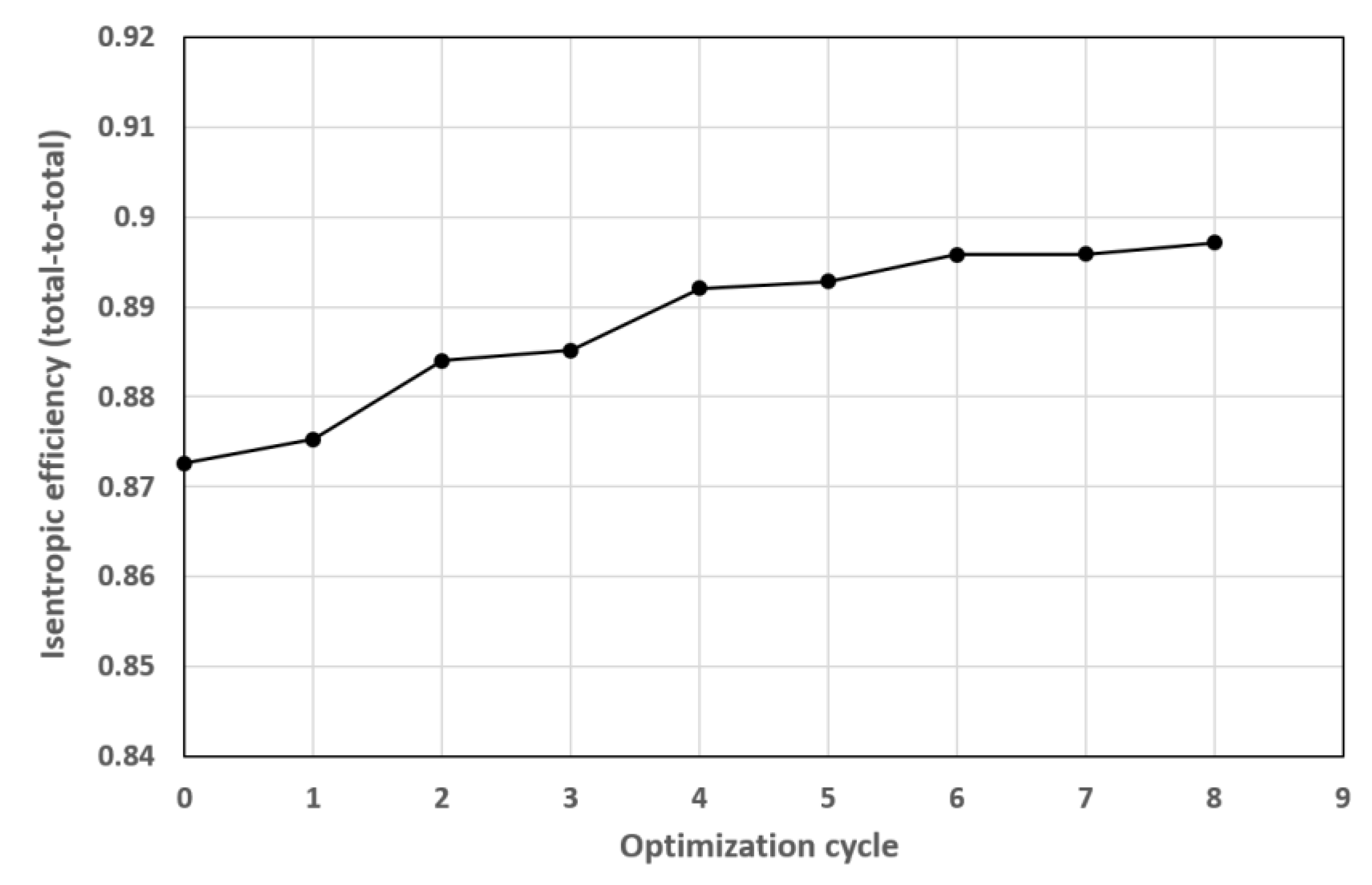
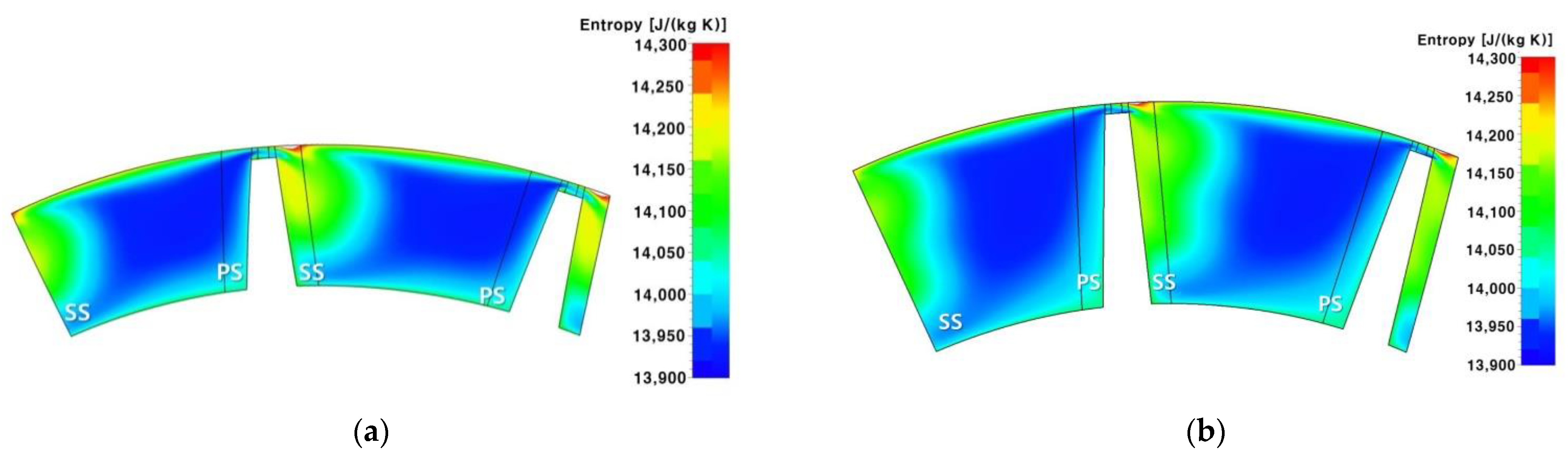
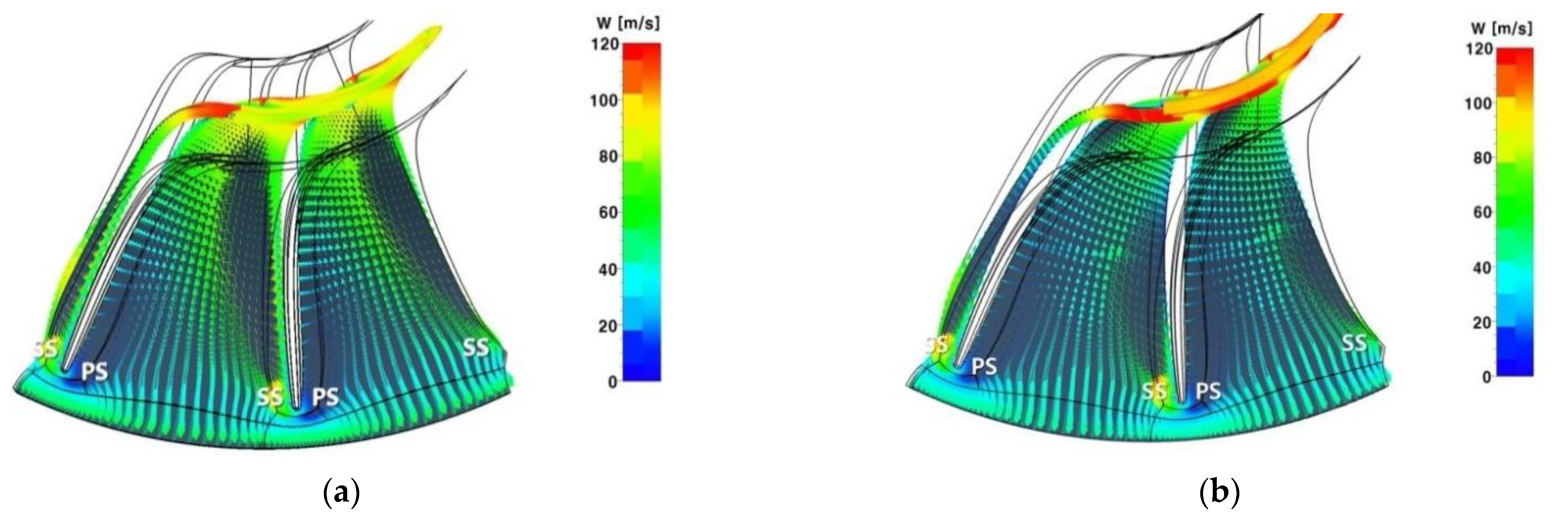
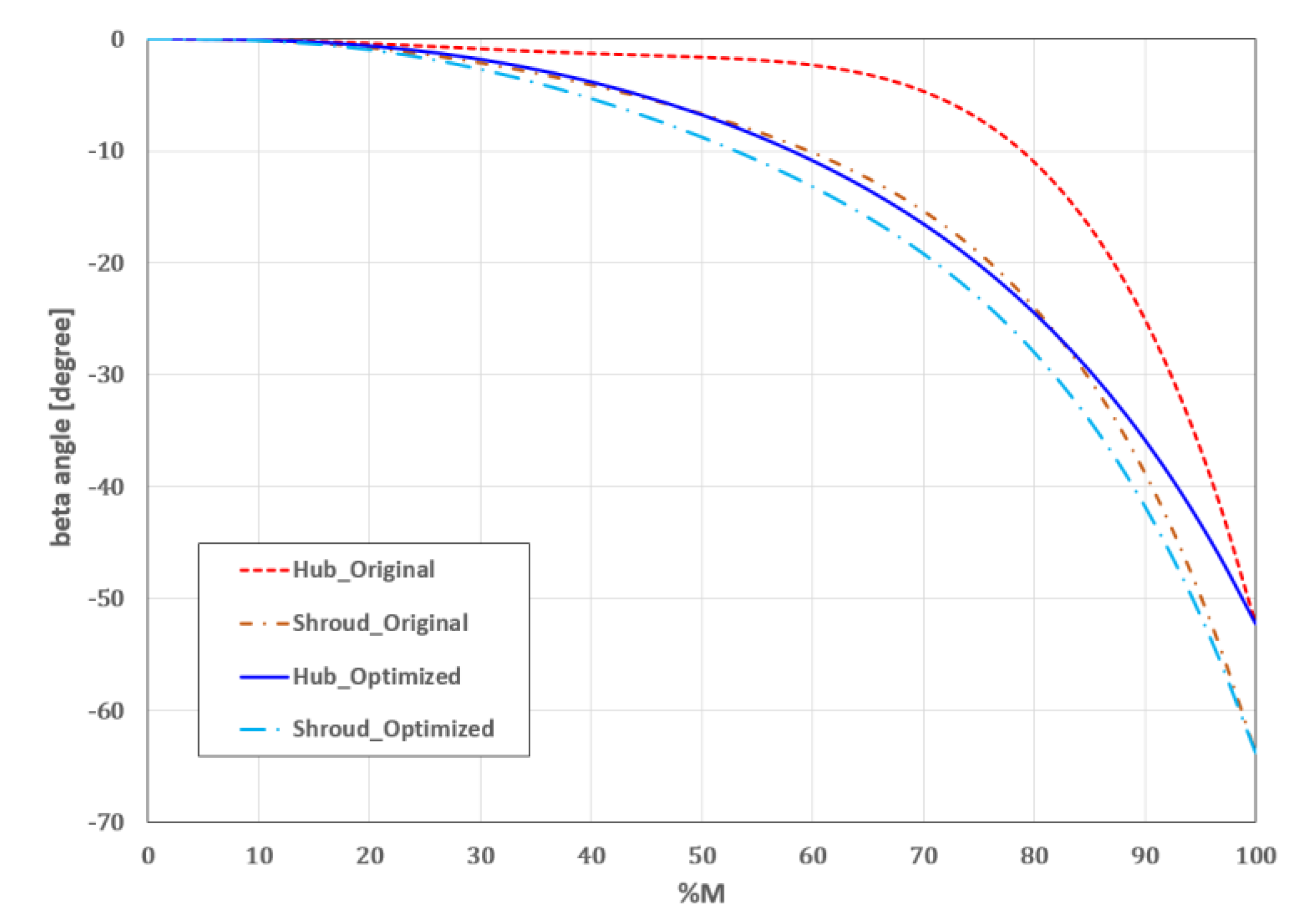
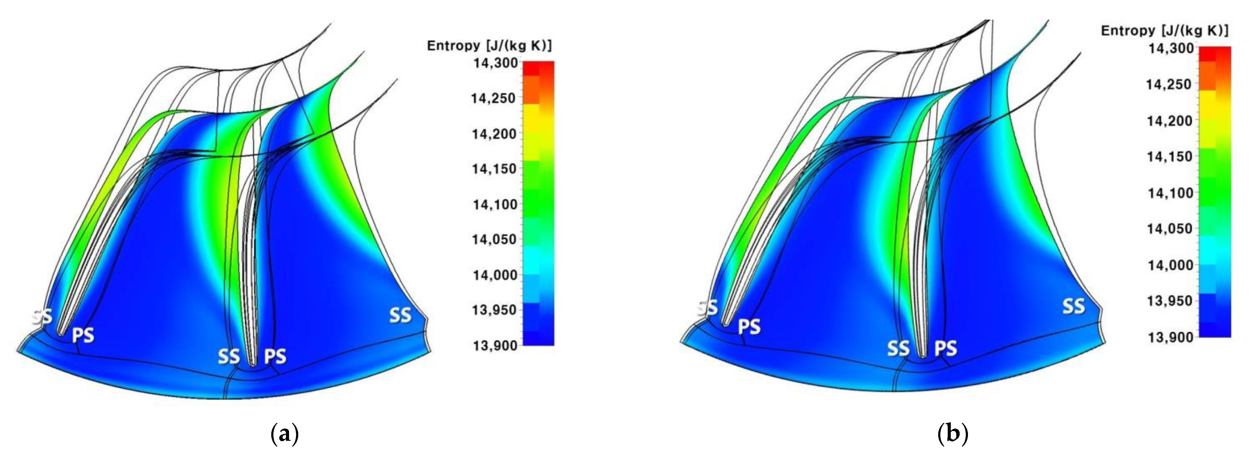
4.3. Optimization Results at Design Point

Figure 14 shows the locations of Planes 1 and 2 in the calculation domain. Plane 1 is the mid-span of the rotor and Plane 2 is the passage area between the blade pressure side and blade suction side. Figure 15 and Figure 16 show the entropy distribution of the rotor, and Figure 17 and Figure 18 show the relative velocity distributions at Planes 1 and 2. As shown in the figures, the entropy of the original model at the suction side of the rotor was larger than that of the optimized model.
Through the optimization, the blade height was increased and the blade β angle was distributed smoothly from the blade leading edge to the trailing edge. The increased rotor blade height induced an increase in the passage area. Therefore, the flow velocity of the optimized model was slightly lower than that of the original model.
As shown in Figure 17, in the original model, the flow area which is not the main passage flow component near the suction blade surface was formed wider than the optimized model. That is, through optimization, the flow of the main passage flow could be smoother than the original model.
As shown in Figure 18, in the case of the original model, a strong tip leakage flow occurs from the pressure blade side to the suction blade side. In the original model, a stronger tip leakage flow occurred in the relatively narrow passage area than in the optimized model, resulting in increased losses and consequently affecting efficiency.

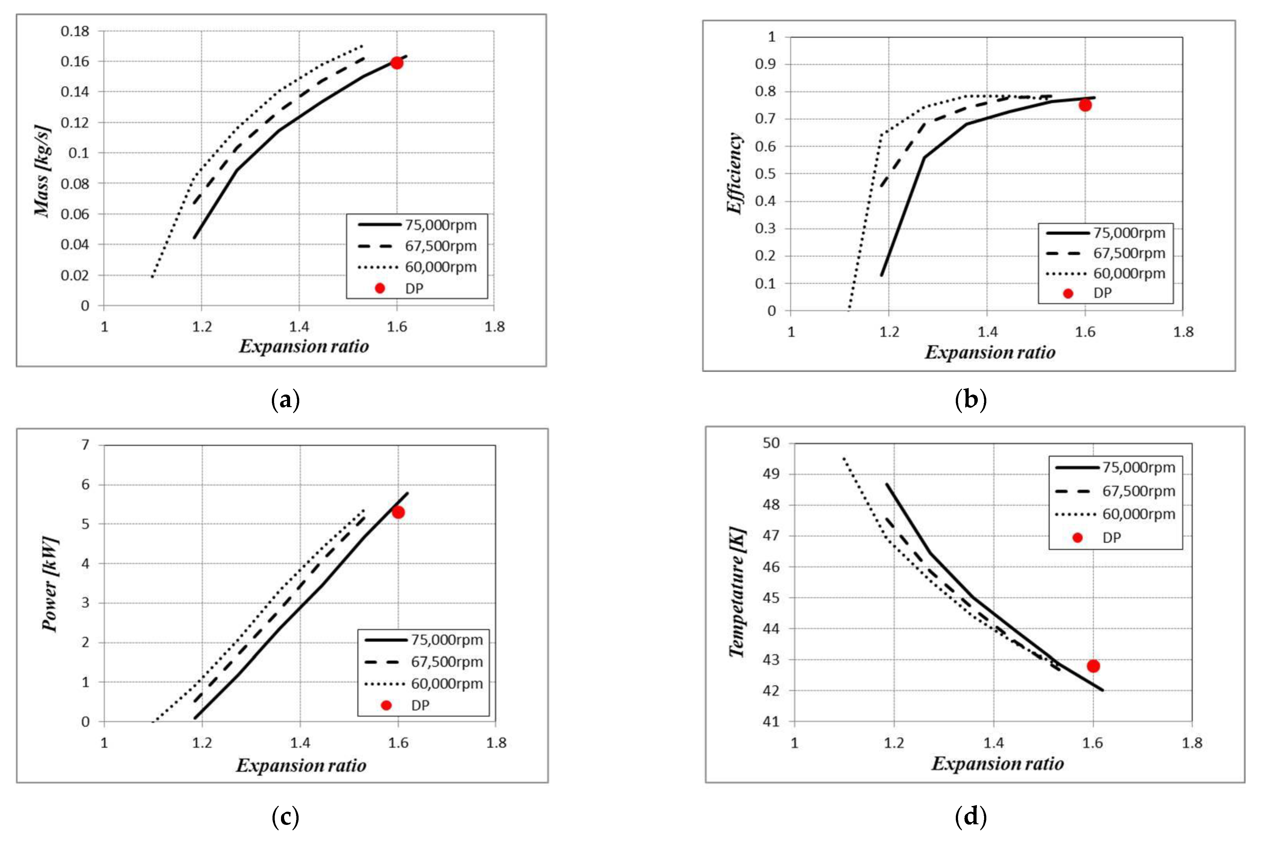
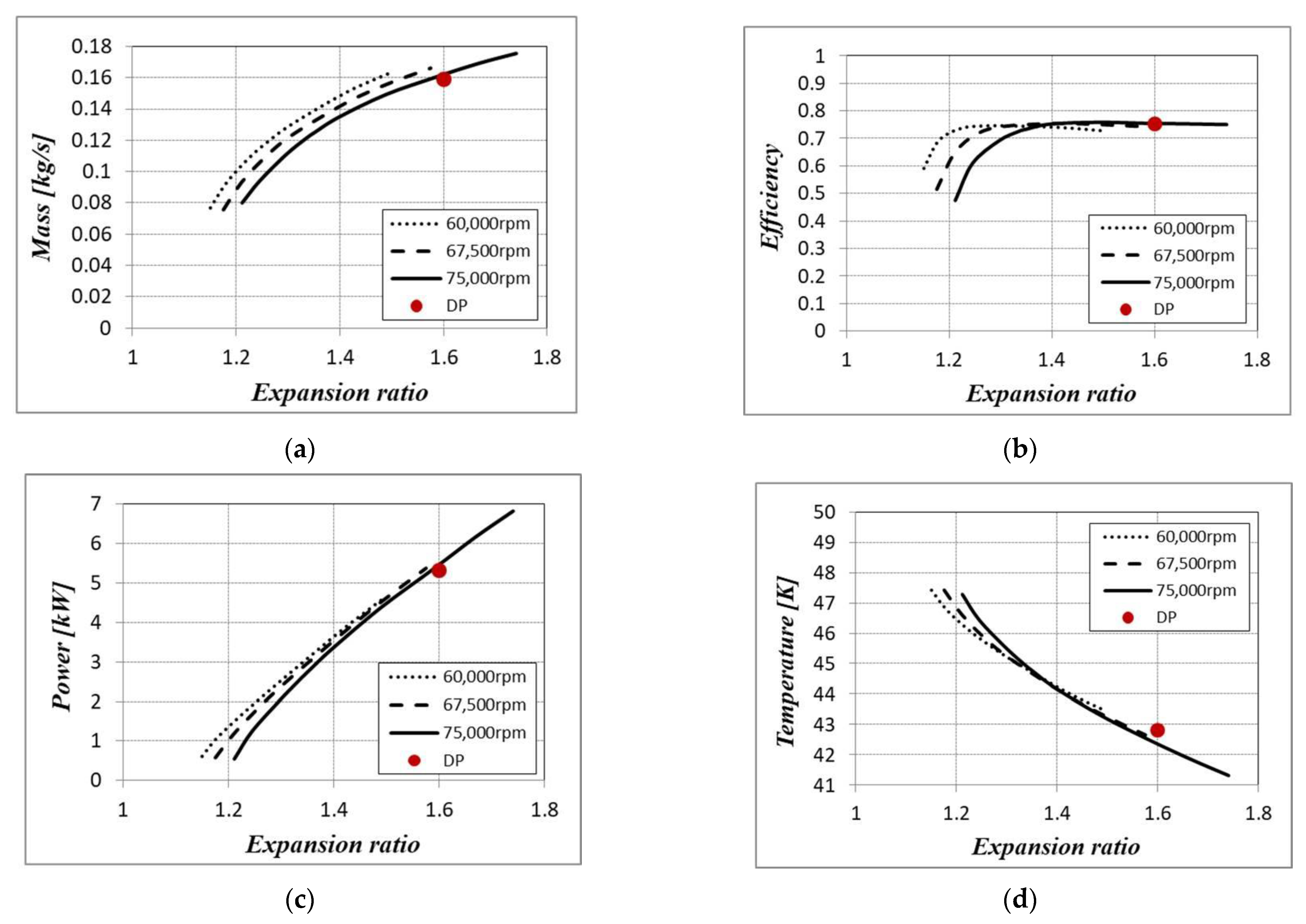
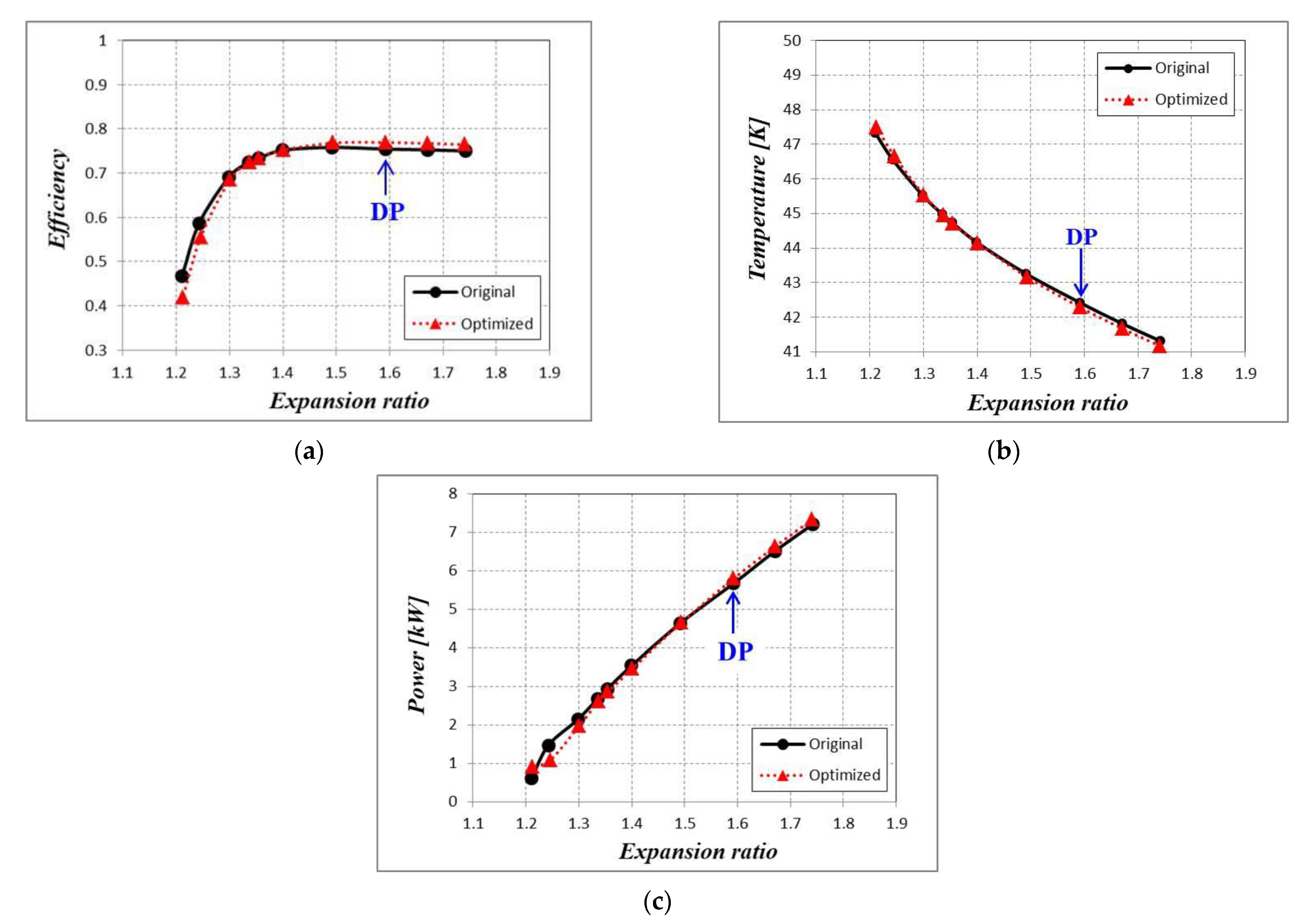
4.4. Comparison of Performance Curve

Figure 19 and Table 6 show a comparison of the performance of the original and optimized models. In Figure 19a, at the design point (DP), it can be seen that the efficiency of the optimized model improved 1.98% compared to that of the original model. Under the condition of an expansion ratio of 1.34 or higher, it was confirmed that the efficiency of the optimization model was improved compared to that of the original model (Table 6). The extra mechanical losses which occur at the volute and the rotor back disk were considered. Figure 19b shows the temperature trends at the expander outlet relative to the expansion ratio. The outlet temperature of the optimized model was 0.32% lower than that of the original model at the design point. Figure 19c shows the relationship between the expansion ratio and the expander output power. At the design point, the power of the optimized model was approximately 2% higher than that of original model.

5. Conclusions

In this study, we introduced a design method for expanders for hydrogen liquefaction plants. Blade optimization was conducted to increase the expander efficiency. The capacity of the developed expander for a hydrogen liquefaction system is 0.5 tons of hydrogen liquefied per day. Based on the cycle analysis results of the hydrogen liquefaction system, the meridional and three-dimensional design of the expander were conducted. To improve the efficiency of the expander, the rotor blade meridional shape and blade β angle were optimized. Through the optimization design, the blade height was increased between the blade leading edge and the trailing edge, and the distribution of the blade β angle was rearranged smoothly. Finally, the optimized expander’s efficiency increased by 1.98% compared to that of the original model. To investigate the reason for this efficiency improvement, a flow analysis was conducted. The entropy distribution on the suction blade surface was smaller in the optimized model than that of the original model. Through the relative velocity distribution, it was found that the optimized model had a smoother main passage flow and smaller tip leakage flow than the original model. Due to the passage area of the optimized model, which is larger than the original model, the effect of the tip leakage flow on the main passage flow could be reduced. It was confirmed that the optimization of the blade β angle, rotor hub, and shroud meridional contour had an effect on improving the efficiency of the cryogenic expander. The efficiency optimization method in this paper can be used as a reference in designing high-efficiency cryogenic expanders in the future.

Author Contributions

Conceptualization, J.S.; methodology, H.L.; software, J.P.; validation, M.P., D.L.; formal analysis, B.C.; investigation, J.B.; writing—original draft preparation, S.K., Y.L. and B.K.; writing—review and editing, H.L. and A.A.; supervision, J.S. All authors have read and agreed to the published version of the manuscript.

Funding

This research was funded by the following projects: the Korea Institute of Energy Technology Evaluation and Planning (KETEP) and the Ministry of Trade, Industry, and Energy (MOTIE) of the Republic of Korea (Project No.: 20188550000200); the Korea Ministry of Land, Infrastructure, and Transportation and the Korean Agency for Infrastructure Technology Advancement (Project No.: KAIA21IHTP-B151613-03); and a National Research Council of Science and Technology (NST) grant funded by the Ministry of Science, ICT and Future Planning, Korea (Grant No. KIMM-NK231D, KIMM-NK231G).

Conflicts of Interest

The authors declare no conflict of interest.

Abbreviations

DOEDesign of experiments
DPDesign point
PSPressure side
RSMResponse surface method
RPMRevolutions per minute
SSSuction side
TPDTons per day
Nomenclature
αAbsolute flow angle [°]
βBlade beta angle, relative flow angle [°]
CAbsolute flow velocity [m/s]
dRotor diameter [mm]
D_tip    Rotor tip diameter [mm]
DsSpecific diameter
ΔDifference
ηEfficiency
hEnthalpy [J/kg]
HxHeat exchanger
InInlet
NsSpecific speed
OutOutlet
ΩRevolution speed [rad/sec]
PrPressure ratio
QFlow rate [㎥/sec]
RRadial
SEntropy [J/kg-K]
TTemperature [K]
URotor tip velocity [m/s]
WRelative velocity [m/s]
ZAxial
Subscript
0Volute
1Nozzle inlet
2Nozzle throat
3Nozzle outlet
4Rotor inlet
5Rotor throat
6Rotor outlet
IsenIsentropic
TTotal
TTTotal to total

References

  1. Simms, J. Fundamentals of Turboexpanders “Basic Theory and Design”; SIMMS Machinery International, Inc.: Santa Maria, CA, USA, 2009. [Google Scholar]
  2. Jumonville, J. Tutorial on cryogenic turboexpanders. In Proceedings of the Thirty-Ninth Turbomachinery Symposium; Texas A&M University, Turbomachinery Laboratories: College Station, TX, USA, 2010; pp. 147–154. [Google Scholar]
  3. Yoshida, S.; Kamioka, Y. Development of a neon cryogenic turboexpander with magnetic bearings. AIP Conf. Proc. 2010, 1218, 895–902. [Google Scholar]
  4. Hirai, H.; Hirokawa, M.; Yoshida, S.; Sano, T.; Ozaki, S. Development of a turbine-compressor for 10 kW class neon turbo-Brayton refrigerator. AIP Conf. Proc. 2014, 1573, 1236–1241. [Google Scholar]
  5. Li, J.; Xiong, L.Y.; Peng, N.; Dong, B.; Wang, P.; Liu, L.Q. Measurement and control system for cryogenic helium gas bearing turbo-expander experimental platform based on Siemens PLC S7-300. AIP Conf. Proc. 2014, 1573, 1743–1749. [Google Scholar]
  6. Ghosh, S.K.; Seshaiah, N.; Sahoo, R.K.; Sarangi, S.K. Design of turboexpander for cryogenic application. Indian J. Cryog. 2015, 2. [Google Scholar]
  7. Ghosh, S.K. Experimental and Computational Studies on Cryogenic Turboexpander. Ph.D. Thesis, National Institute of Technology, Rourkela, India, 29 July 2008. [Google Scholar]
  8. Choudhury, B.K. Design and Construction of Turboexpander Based Nitrogen Liquefier. Ph.D. Thesis, National Institute of Technology, Rourkela, India, 24 December 2013. [Google Scholar]
  9. Song, P.; Sun, J.; Wang, K. Swirling and cavitating flow suppression in a cryogenic liquid turbine expander through geometric optimization. J. Power Energy 2015, 229, 628–646. [Google Scholar] [CrossRef]
  10. Huang, N.; Li, Z.; Zhu, B. Cavitating flow suppression in the draft tube of a cryogenic turbine expander through runner optimization. Processes 2020, 8, 270. [Google Scholar] [CrossRef] [Green Version]
  11. Moustapha, H.; Zelesky, M.F.; Baines, N.C.; Japikse, D. Axial and Radial Turbines; Concepts ETI, Inc.: White River Junction, VT, USA, 2003. [Google Scholar]
  12. Cho, S.-Y.; Choi, B.-S.; Lim, H.-S. Study of pressure loss according to the cross-sectional shapes of volute on radial turbine. J. Korean Soc. Power Syst. Eng. 2019, 23, 55–64. [Google Scholar] [CrossRef]
  13. Barton, R.R. Tutorial: Simulation Metamodeling. In Proceedings of the 2015 Winter Simulation Conference, IEEE, Huntington Beach, CA, USA, 6–9 December 2015; pp. 1765–1779. [Google Scholar]
  14. Karmoker, J.R.; Hasan, I.; Ahmed, N.; Saifuddin, M.; Reza, M.S. Development and Optimization of Acyclovir Loaded Mucoadhesive Microspheres by Box -Behnken Design. Dhaka Univ. J. Pharm. Sci. 2019, 18, 1–12. [Google Scholar] [CrossRef]
  15. Greenfield, T.; Metcalfe, A.V. Design and Analysis Your Experiment with MINITAB; John Wiley & Sons Ltd.: West Sussex, UK, 2010. [Google Scholar]
  16. Montgomery, D.C. Introduction to Statistical Quality Control; John Wiley & Sons Ltd.: Hoboken, NJ, USA, 2005. [Google Scholar]
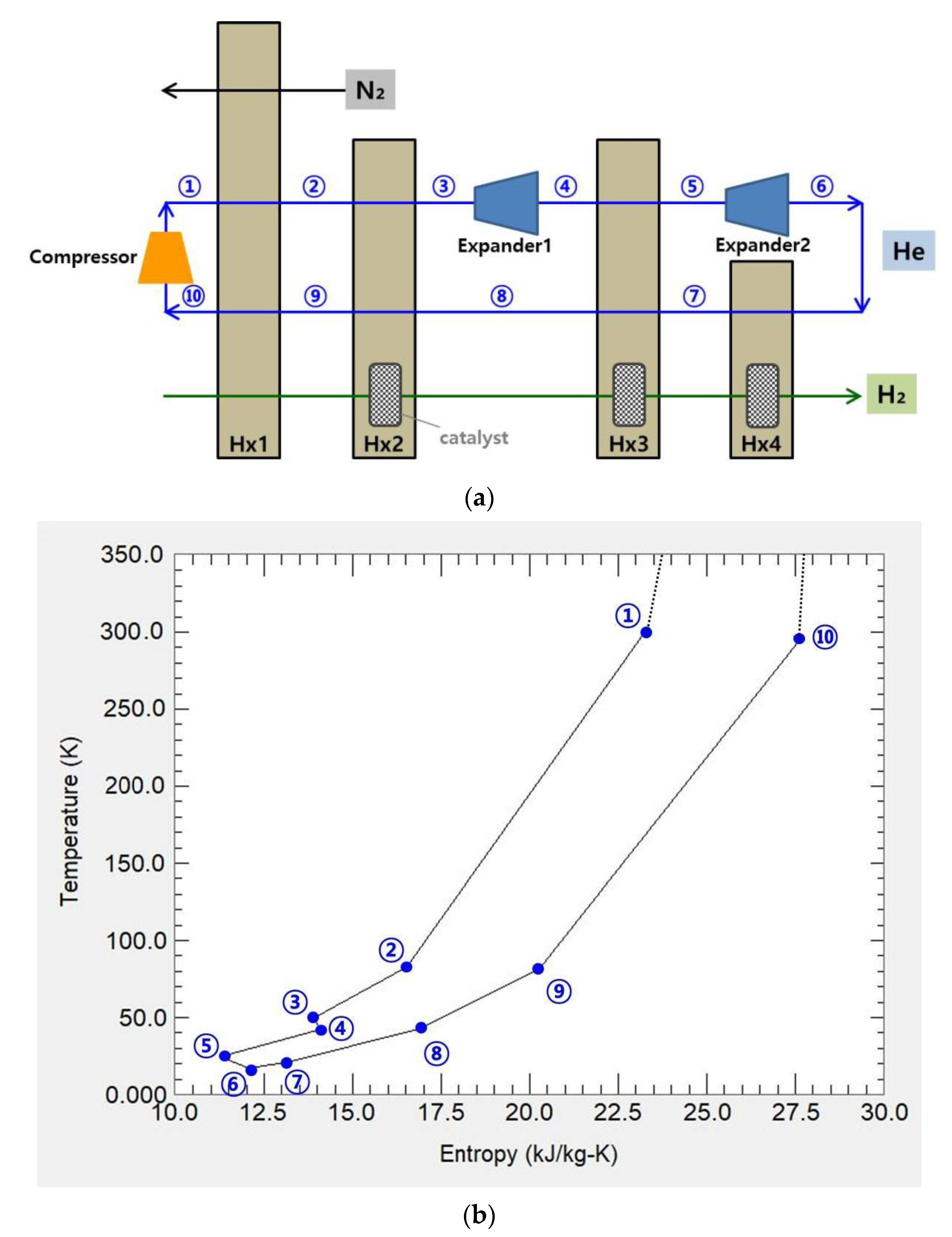
Figure 1. The 0.5-TPD class hydrogen liquefaction plant: (a) schematic of hydrogen liquefaction plant and (b) T–s diagram of hydrogen liquefaction plant.
Applsci 12 01411 g001
Figure 2. Meridional view of expander.
Applsci 12 01411 g002
Figure 3. Velocity triangles at design points: (a) rotor inlet (incidence angle −26.74°) and (b) rotor outlet (deviation angle 22.8°).
Applsci 12 01411 g003
Figure 4. Performance prediction curves from meanline analysis: (a) expansion ratio vs. mass flow rate; (b) expansion ratio vs. efficiency; (c) expansion ratio vs. power; (d) expansion ratio vs. expander outlet temperature.
Applsci 12 01411 g004
Figure 5. Generated 3D geometry of nozzle and rotor.
Applsci 12 01411 g005
Figure 6. Grid independence test for the numerical analysis.
Applsci 12 01411 g006
Figure 7. Performance prediction curves from numerical analysis: (a) expansion ratio vs. mass; (b) expansion ratio vs. efficiency; (c) expansion ratio vs. power; (d) expansion ratio vs. expander outlet temperature.
Applsci 12 01411 g007
Figure 8. Flowchart of response surface meta-model-based optimization methodology.
Applsci 12 01411 g008
Figure 9. Hub and shroud meridional contours controlled by Bezier curves.
Applsci 12 01411 g009
Figure 10. Blade β angle distributions controlled by Bezier curves.
Applsci 12 01411 g010
Figure 11. Isentropic total-to-total efficiency of expander by shape optimization without assuming the extra mechanical losses.
Applsci 12 01411 g011
Figure 12. Comparison of blade β angle distributions obtained by shape optimization.
Applsci 12 01411 g012
Figure 13. Comparison of hub and shroud meridional contours obtained by shape optimization.
Applsci 12 01411 g013
Figure 14. Locations of Planes 1 and 2 in the CFD domain.
Applsci 12 01411 g014
Figure 15. Comparison of entropy distribution at mid-span of the rotor (Plane 1): (a) original model and (b) optimized model.
Applsci 12 01411 g015
Figure 16. Comparison of entropy distribution at Plane 2: (a) original model and (b) optimized model.
Applsci 12 01411 g016
Figure 17. Comparison of relative velocity distribution at Plane 1: (a) original model and (b) optimized model.
Applsci 12 01411 g017
Figure 18. Comparison of relative velocity distribution at Plane 2: (a) original model and (b) optimized model.
Applsci 12 01411 g018
Figure 19. Performance comparisons between the original model and optimized model: (a) expansion ratio vs. efficiency; (b) expansion ratio vs. expander outlet temperature; (c) expansion ratio vs. expander power.
Applsci 12 01411 g019
Table 1. Components involved in each process of the T–s diagram.
Process @
T–s Diagram
Component
①-②Heat exchanger 1
②-③Heat exchanger 2
③-④Expander 1
④-⑤Heat exchanger 3
⑤-⑥Expander 2
⑥-⑦Heat exchanger 4
⑦-⑧Heat exchanger 3
⑧-⑨Heat exchanger 2
⑨-⑩Heat exchanger 1
⑩-①Compressor with cooler
Table 2. Operation conditions of Expanders 1 and 2.
ParameterUnitExpander 1
(③–④)
Expander 2
(⑤–⑥)
Pt_inbar9.765.98
Tt_inK49.124.8
Pt_outbar6.11.62
Tt_outK42.817
Pr-1.63.69
Efficiency%74.776.3
PowerkW5.326.2
Table 3. Preliminary design results for Expander 1.
NsUnit0.20.30.40.50.60.70.80.91.00.392
Efficiency-0.760.810.850.870.870.840.80.720.610.85
RPM-38,19157,28676,38295,477114,573133,668152,764171,859190,95575,000
PowerkW5.45.76.06.16.16.05.65.14.36.0
Ds-10.06.675.04.03.332.862.52.222.05.09
D_tipmm105.5970.3952.842.2435.230.1726.423.4621.1253.77
U_tipm/s211.15211.15211.15211.15211.15211.15211.15211.15211.15211.15
Table 4. Meanline design results.
ParameterUnitDimension
RPM-75,000
Number of nozzles-17
Nozzle inlet radius (N1)mm36.5
Nozzle outlet radius (N2)mm29.5
Nozzle heightmm3.3
Nozzle outlet blade angle°76.21
Number of rotors-14
Rotor inlet radius (R1)mm26
Rotor outlet shroud radius (R2)mm13.2 + 0.3
Rotor outlet hub radius (R3)mm8.4
Rotor outlet blade angle°−60
Table 5. Design parameters and metamodel in each optimization cycle.
CycleDesign ParametersMetamodel
1blade
β angle
U = 0.872630 0.000602   β H 3 0.001696   β H 4 + 0.000415   β S 3 + 0.000553   β S 4                                                 + 0.000022   β H 3 β H 3 + 0.000134   β H 4 β H 4 + 0.000015   β S 3 β S 3                                                 + 0.000084   β S 4 β S 4 0.000050   β H 3 β H 4 0.000017   β H 3 β S 3                                                   0.000003   β H 3 β S 4 0.000040   β H 4 β S 3 0.000188   β H 4 β S 4                                                 + 0.000112   β S 3 β S 4
2meridional
contours
U = 0.875270 0.003063   Z H 2 0.001480   R H 3 + 0.003210   Z S 2 + 0.001197   R S 3                                                 0.000112   Z H 2 Z H 2 0.000010   R H 3 R H 3 0.000145   Z S 2 Z S 2                                                   0.000180   R S 3 R S 3 + 0.000207   Z H 2 R H 3 + 0.000153   Z H 2 Z S 2                                                 0.000100   Z H 2 R S 3 0.000222   R H 3 Z S 2 0.000020   R H 3 R S 3                                                 + 0.000170   Z S 2 R S 3
3blade
β angle
U = 0.884060 0.000268   β H 3 0.001175   β H 4 + 0.000102   β S 3 + 0.000020   β S 4                                                 0.000064   β H 3 β H 3 0.000192   β H 4 β H 4 0.000044   β S 3 β S 3                                                   0.000162   β S 4 β S 4 0.000140   β H 3 β H 4 + 0.000080   β H 3 β S 3                                                 + 0.000095   β H 3 β S 4 + 0.000055   β H 4 β S 3 + 0.000190   β H 4 β S 4                                                 0.000060   β S 3 β S 4
4meridional
contours
U = 0.885210 0.002624   Z H 2 0.001767   R H 3 + 0.002823   Z S 2 + 0.001001   R S 3                                                 0.000214   Z H 2 Z H 2 + 0.000050   R H 3 R H 3 0.000225   Z S 2 Z S 2                                                   0.000099   R S 3 R S 3 + 0.000005   Z H 2 R H 3 + 0.000242   Z H 2 Z S 2                                                 + 0.000095   Z H 2 R S 3 0.000023   R H 3 Z S 2 0.000022   R H 3 R S 3                                                 0.000050   Z S 2 R S 3
5blade
β angle
U = 0.892050 + 0.000054   β H 3 0.000543   β H 4 0.000093   β S 3 0.000231   β S 4                                                 0.000071   β H 3 β H 3 0.000583   β H 4 β H 4 + 0.000030   β S 3 β S 3                                                   0.000016   β S 4 β S 4 0.000507   β H 3 β H 4 + 0.000073   β H 3 β S 3                                                 + 0.000067   β H 3 β S 4 + 0.000132   β H 4 β S 3 + 0.000340   β H 4 β S 4                                                 + 0.000005   β S 3 β S 4
6meridional
contours
U = 0.892940 0.001352   Z H 2 0.001308   R H 3 + 0.001674   Z S 2 + 0.000508   R S 3                                                 0.000555   Z H 2 Z H 2 0.000188   R H 3 R H 3 0.000321   Z S 2 Z S 2                                                   0.000192   R S 3 R S 3 0.000210   Z H 2 R H 3 + 0.000367   Z H 2 Z S 2                                                 + 0.000183   Z H 2 R S 3 + 0.000200   R H 3 Z S 2 + 0.000153   R H 3 R S 3                                                 0.000165   Z S 2 R S 3
7blade
β angle
U = 0.895790 + 0.000402   β H 3 + 0.000905   β H 4 0.000169   β S 3 0.000332   β S 4                                                 0.000215   β H 3 β H 3 0.001522   β H 4 β H 4 0.000081   β S 3 β S 3                                                   0.000123   β S 4 β S 4 0.001088   β H 3 β H 4 + 0.000100   β H 3 β S 3                                                 + 0.000218   β H 3 β S 4 + 0.000233   β H 4 β S 3 + 0.000660   β H 4 β S 4                                                 0.000065   β S 3 β S 4
8meridional
contours
U = 0.895840 0.000051   Z H 2 0.000798   R H 3 + 0.000898   Z S 2 + 0.000019     R S 3                                                 0.000257   Z H 2 Z H 2 0.000155   R H 3 R H 3 0.000118   Z S 2 Z S 2                                                   + 0.000011     R S 3   R S 3 0.000070   Z H 2 R H 3 + 0.000135   Z H 2 Z S 2                                                 0.000023   Z H 2   R S 3 + 0.000120   R H 3 Z S 2 + 0.000060   R H 3   R S 3                                                 + 0.000030   Z S 2   R S 3
Table 6. Efficiency and outlet temperature comparisons between original and optimized models.
Expansion
Ratio
EfficiencyΔEfficiency
[%] *
Outlet Temperature [K]ΔTemperature
[%] *
OriginalOptimizedOriginalOptimized
1.740.7500.7641.941.30641.1670.34
1.670.7520.7671.9441.81341.6740.33
1.59 (DP)0.7540.7691.9842.41542.2810.32
1.490.7580.7681.3243.25243.1610.21
1.400.7520.7520.0844.16444.1440.05
1.350.7330.7340.144.7344.7180.03
1.340.7230.7250.1544.97344.9480.06
1.300.6900.685−0.7345.52845.5260.00
1.240.5860.555−5.2146.56446.66−0.21
1.210.4660.419−10.0747.31947.488−0.36
* Comparisons were conducted based on the original model.
Publisher’s Note: MDPI stays neutral with regard to jurisdictional claims in published maps and institutional affiliations.

