Abstract
There are two major types of iron ore deposits in the Pilbara Province of Western Australia—banded iron formation (BIF)-hosted iron ore deposits and bedded iron deposits (BID), respectively, named martite–goethite and martite–microplaty hematite and the channel iron deposits (CID). These deposits consist mainly of iron oxides such as magnetite, hematite and goethite; the latter have been subdivided into vitreous and ochreous goethite. Combining spectral scanning of diamond drill core, drill chips and pulps collected from these deposits provides a rapid and relatively inexpensive means of assessing the potential mineral makeup within a deposit to make informed qualitative decisions. Additionally, the full width half maximum (FWHM) of the 900 nm 6A1→4T1 crystal field absorption feature within the goethite-dominated region is shown to be related to the type of goethite, namely ochreous and vitreous. The assessment capabilities of the combined metrics are presented in a visual format named as the iron boomerang because of its distinctive manifold. This provides the identification of at least two spectral endmembers comprised of hematite and vitreous goethite, the identification of samples that are moving from a pure hematite to mixed hematite/goethite and lastly into a goethite-dominant-driven regime.
Keywords:
iron oxide; hyperspectral; crystal field absorption; hematite; goethite; ochreous; vitreous; Hamersley Basin; Rocklea Dome; Pilbara; martite 1. Introduction
The use of hyperspectral reflectance spectra (“spectral data”) in the iron ore resources industry is well established and continues to be a valuable tool to aid orebody characterisation, mineral classification, and quantification [1,2,3,4]. The use of spectral data for characterisation purposes is dependent on the wavelength region in which the reflectance spectra were collected. This has led to spectral region-specific metrics that are used to leverage the strength of each spectral region and, in many cases, is deposit specific [1,5,6,7]. In the combined visible (VIS), near-infrared (NIR) and short-wave infrared (SWIR) between 350 and 2500 nm, the 1300–2500 nm spectral region has alteration mineral assemblages associated with hydrothermal base and precious metal deposits which can often be defined by the absorption features present [8,9,10,11,12,13], while absorptions in the VIS and NIR between 350 and 1300 nm can be used to infer iron-bearing minerals [2,14,15].
At much longer wavelengths in the thermal infrared (TIR) spectral region, absorptions between 6000 and 14,000 nm are used to assist in mineral species differentiation due to overlapping and confounding absorptions, such as carbonates and chlorites, in the SWIR as well as the identification of minerals that do not exhibit any identifiable absorptions in the VIS, NIR and SWIR such as quartz and feldspars [13,16,17].
The two major types of iron ore deposits in the Pilbara Province of Western Australia are banded iron formation (BIF)-hosted iron ore deposits and bedded iron deposits BID, respectively, named martite–goethite and martite–microplaty hematite and channel iron deposits (CID), as described in [18]. Ochreous goethite has been defined as yellow in colour and powdery to friable, vitreous goethite is dark red-brown to black in colour, with a relative hardness ranging from medium to hard; brown goethite is light to dark brown in colour, with a medium to hard hardness [19]. In a typical goethite, the Moh hardness scale has a range of 5–5.5 but the yellow ochreous goethite is much lower due to its porosity.
The collection of spectral data from exploration samples or laboratory prepared samples is fast and cost-effective and can provide a greater insight into the iron oxide mineral and mineral assemblages of iron ore bodies. The spectral data might be collected from rotary core (RC) chip samples collected via a diamond core scanned with the HyLoggerTM [20,21,22] or Corescan HSI [23], or from samples prepared as pulps prior to geochemical assay using laboratory spectrometers. Processing the spectral data with a suite of spectral metrics allows a fast overview to be produced, which can aid further exploration decisions, free up field geologists, and potentially assist in ongoing mining operations, for example, by informing material handling indices [24].
The interpretation of ore and waste mineral assemblages present in each iron ore-specific spectral dataset will, as previously noted, be dependent on the wavelength regions and instrument specifications available. Shale-containing clay minerals can be established via SWIR spectral metrics, chert and high-silica samples can be identified with TIR spectral metrics, while the VNIR can be used to establish the presence of hematite/magnetite and goethite. In the latter case, the crystal field absorption (CFA) 6A1→4T1 at approximately 900 nm (F900) [25], shown in Figure 1, has been used to infer proportions of hematite/magnetite and goethite [5], vitreous and ochreous goethite discrimination and Fe content [1,26]. The F900 is of particular interest as it is a large and well-resolved absorption feature. This study focuses primarily on the F900 absorption feature and more specifically on how calculation of the full width half maximum (FWHM) of the feature, when combined with the wavelength of the point of maximum absorption of the F900 absorption wavelength, adds a strong qualitative aspect to spectral datasets collected in BID and CID formations.
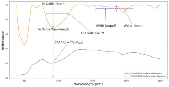
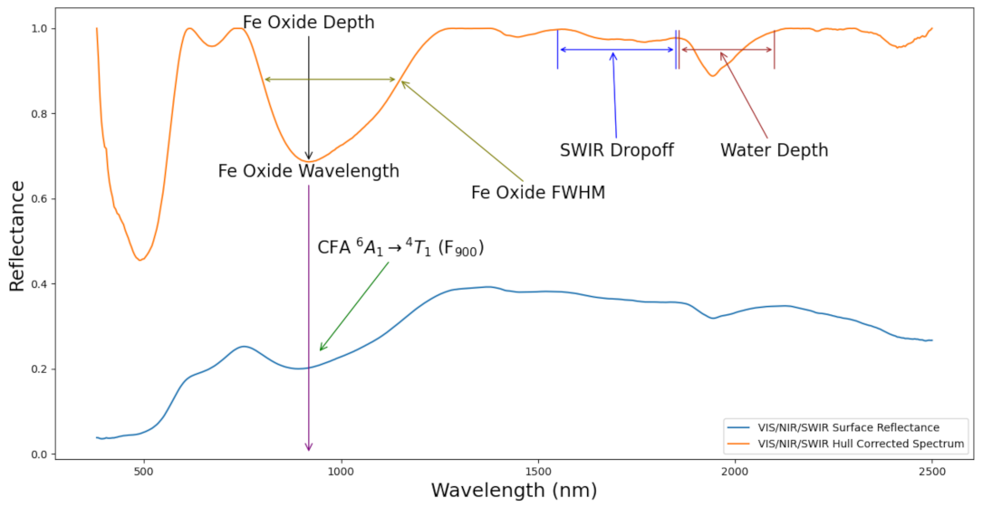
Figure 1.
A surface reflectance goethite sample (blue spectrum) showing the 6A1→4T1 (F900) crystal absorption feature at approximately 900 nm. The upper spectrum in orange is the hull-corrected spectrum. The hull-corrected F900 feature is used to define the point at which the deepest absorption value occurs and defines the Fe oxide wavelength, Fe oxide FWHM and Fe oxide depth spectral metrics. The wavelength region between 1550 and 1850 nm is the region where a local hull correction is performed, and the maximum depth recorded as the SWIR dropoff metric. The region between 1850 and 2100 nm also uses a local correction to calculate the maximum depth and is recorded as the water depth. See Figure 2 for an example of the iron boomerang scatterplot.
The manifold is formed by plotting the F900 wavelength versus the FWHM of the F900 and is herein referred to as the iron boomerang due to its distinct shape. This shape is not necessarily evident in sparse spectral datasets, but the findings are still applicable. Visualising the calculated F900 wavelength versus F900 FWHM data in the iron boomerang allows the user to immediately see the general composition of the dataset in terms of hematite/magnetite and goethite and, as will be shown, the magnitude of the F900 FWHM feature in the goethite-dominated region, which can provide a level of vitreous and ochreous goethite discrimination.
2. Methods
All the accompanying spectral metrics used herein make use of a hull quotient [27], referred herein as hull corrected, to leverage absorption features of a given spectrum. All of the spectral metrics and masking of samples used in this study were calculated in the CSIRO-developed The Spectral Geologist (TSGTM) software [28,29] version 8.0.7.4. It is noted that a user can use other software or programming language to calculate the spectral metrics. Unless stated otherwise, the “Pfit” function in TSGTM was used to perform hull correction and to fit 10th-order polynomials across the given spectral regions. A 10th-order polynomial was selected to ensure a good fit as we are not interested in defining the minimum applicable polynomial order (see Table 1).

Table 1.
The spectral metrics used in this study. The calculation of the metrics was performed in the CSIRO-developed TSGTM software. The last column “Usage” shows the general purpose of the metric.
With reference to Figure 1 and Table 1, the first spectral metric is the estimated wavelength at which the deepest absorption occurs (Fe oxide wavelength), and the second is the estimated FWHM (Fe oxide FWHM) of the hull-corrected 900 nm 6A1->4T1 CFA absorption feature. The location of the Fe oxide wavelength is shown in Figure 1 as the purple downward arrow. Of note here is the apparent offset between the minimum point of absorption between the reflectance spectrum and that of the hull-corrected spectrum which is due to distorting the effect of the background hull [30]. The Fe oxide FWHM is the width of the feature (shown in olive in Figure 1 and described in Table 1) as calculated at a depth that is one half of the maximum feature depth.
To present the spectral metrics in the iron boomerang form is simply a matter of plotting the Fe oxide wavelength versus the Fe oxide FWHM metric. An example of the iron boomerang can be seen in Figure 2 in the results section and whose properties will be discussed further at that point.

Figure 2.
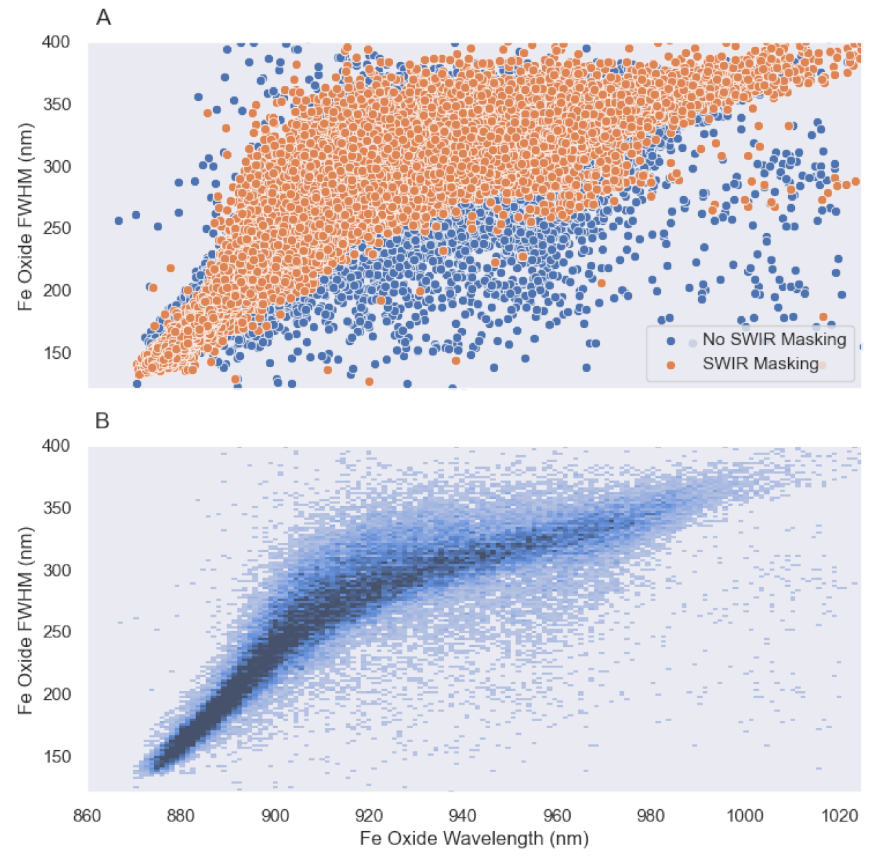
(A) shows the plot of the Fe oxide wavelength versus the Fe oxide FWHM for both the complete dataset (labelled as no SWIR masking) and the dataset after masking for SWIR alteration minerals (labelled as SWIR masking) which leads to a suppression of the Fe oxide FWHM values. (B) shows a density plot comprising 120 × 400 cells giving a spectral resolution of approximately 1.4 nm × 0.7 nm and demonstrates a typical density distribution of the iron boomerang for dense datasets. (B) is applied to the “no SWIR masking” data in (A).
An additional metric included in this study is the maximum depth of the F900 absorption feature (see Figure 1 and Table 1) that is primarily used here for visual aesthetics but it does, however, increase with decreasing hematite and increasing goethite. The depth of the 1900 nm water feature between 1880 and 2100 nm (water depth) is used to highlight the samples originating from the CID spectral data (not shown in Figure 1). Lastly, an increase in the depth of a local continuum removed spectra between 1550 and 1850 nm (SWIR dropoff) which aligns with increasing vitreous goethite. The region in which the latter is applied is shown in Figure 1 between the two blue lines and labelled SWIR dropoff.
3. Materials
The spectral data used in this study are sourced from several CSIRO-led collaborations with the iron ore industry. They total seven individual spectral datasets from two different deposit types. Namely, RC chips spectrally scanned with the HyLoggerTM from the Rocklea Dome CID [1,6,31,32] and a combination of RC chips, diamond core and pulps from across the Hamersley Basin in Western Australia. The HyLoggerTM has two spectrometers in the 380–2500 nm spectral region. The first is a silicon-detector grating spectrometer covering the 380–1072 nm spectral region and the second is an InSb-detector FTIR (Fourier Transform Infrared) spectrometer covering the 1072–2500 nm spectral region. The HyLoggerTM produces spectral samples approximately every 1 cm when used with drillcore or a total of 3 samples per chip bin averaged to a single spectrum when used with chips.
The combined spectral dataset is comprised of 1 pulp dataset (BIF), 2 diamond core (BID) and 4 RC chip datasets, with the latter comprised of one CID and three BID formations (see Table 2). The Rocklea Dome dataset is publicly available; however, the remaining 6 datasets are sourced from company datasets and are subject to intellectual property constraints. In the latter case, it is not possible to identify the spectral dataset owners nor to specifically geolocate the datasets within the Hamersley Basin. All the data have been, if not originally, spectrally resampled to a 1 nm spectral sampling between 380 and 2500 nm.
Table 2.
The seven spectral data sources used in this study and the total number of spectral samples for each dataset prior to any masking.
Drillcore is placed into core trays containing 3–4 rows, dependent on the core tray, with a length of 1 m per row. The core is first cleaned prior to scanning and then the tray is placed on the HyLoggerTM x-y translation table for scanning and surface reflectance determination. In a similar manner, RC chip samples are placed into a tray comprised of a number of individual chip buckets where each chip bucket sample is representative of the user chip meterage. The HyLoggerTM, in this case, is moved on the x-y translation table from bucket to bucket collecting 3 spectral samples per bucket and averaging those into a singular surface reflectance value.
Prior to showing results, it is prudent to remind the reader of the spectral absorption wavelengths expected in the Hamersley Basin spectral datasets. Table 3 shows the mineral in question in column 1 and the corresponding absorption wavelengths in column for a given study (column 3). It is noted that hematite is noted as occurring below 890 nm and goethite above 890 nm. The kaolinite absorption feature is also shown since it is used to reduce the impact of alteration minerals that may be present in the datasets. Another mineral that might impact the SWIR but not shown in Table 3 are carbonates with absorption features approximately located at 2310–2320 nm.
Table 3.
Wavelength positions of hematite, goethite and kaolinite established from a number of different studies. It is important to note that some differences are due to differing spectral regions used in continuum corrected spectra. The hematite and goethite absorption wavelengths presented are adapted from Table I of [25].
4. Results
The results are designed to highlight various properties associated with the iron boomerang. More than 62,000 data points were available for plotting; however, the figures do not generally show results with the total number of available samples as a level of masking is first applied to many of the plots to remove samples that are affected by potential alteration minerals such as kaolinite and carbonate. The masking of alteration minerals in the SWIR was achieved by selecting only samples that the SWIR The Spectral Assistant (TSA) algorithm [28] identified as “aspectral” in the mineral classification estimation. In this case, the term refers to spectra that do not exhibit any appreciable SWIR absorptions. After masking for absorptions indicative of SWIR alteration minerals, a total of 39,000 points were left. It is noted that no other analysis such as geochemistry was used in this study. However, the drillcore and RC chips used were visually inspected to ascertain the iron mineral types.
The plot of the Fe oxide wavelength versus the Fe oxide FWHM for both the complete dataset (labelled as no SWIR masking) and the dataset after masking for SWIR alteration minerals (labelled as SWIR masking) shows the presence of weathering minerals, primarily kaolinite in the seven datasets and small amounts of siderite (1000 nm) and leads to a suppression of the Fe oxide FWHM values (Figure 2A). If the kaolinite amounts in each spectrum are significant, then a small absorption located at approximately 960 nm [37] can be observed, which can also impact the Fe oxide wavelength, leading to a slight clustering of kaolinite-affected values at approximately 960 nm and below an Fe oxide FWHM value of 250 nm.
While the SWIR masked data points are much closer in appearance to an iron boomerang shape, the underlying distribution (Figure 2A) is a product of a dense dataset that is affected by overplotting. Overplotting refers to a lack of transparency in the plot markers so that regions that may only have very few points in them effectively hide the distribution of the data.
To better highlight the distribution of data points in the iron boomerang, and the origin of the name, a density plot for the “no SWIR masking” data (Figure 2A) was used and subsequently displayed in Figure 2B. The density plot comprises 120 × 400 cells, giving a spectral resolution of approximately 1.4 nm × 0.7 nm and demonstrates a typical density distribution of the iron boomerang for dense datasets (Figure 3). As noted previously the effect of kaolinite can be seen by the portion of samples showing an Fe oxide wavelength of approximately 960 nm and below an Fe oxide FWHM of 250 nm. As previously noted, samples located between 1000 and 1020 nm and with Fe oxide FWHM values less than 350 nm tend to have siderite present.
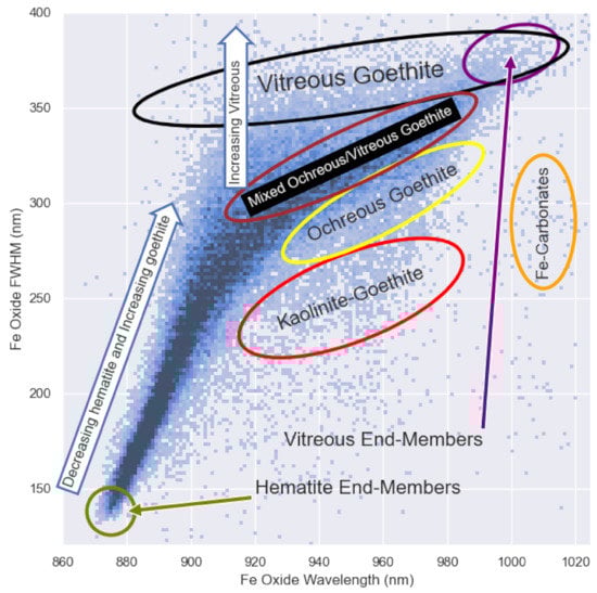
Figure 3.
The density plot of the complete dataset with no SWIR masking is shown and outlines the general composition and placement of key locations within the iron boomerang. At each end are two spectral endmembers comprised of hematite around a Fe oxide wavelength of 870 nm and Fe oxide FWHM of approximately 140 nm and vitreous goethite located approximately at a Fe oxide wavelength of >980 nm and Fe oxide FWHM of >370 nm. As the iron boomerang is traversed from left to right and bottom to top the proportion of hematite to goethite decreases toward a more goethite-dominated region at wavelengths greater than approximately 920 nm. As the Fe oxide FWHM increases within the goethite-dominated region, a move from more ochreous goethite to greater proportions of vitreous goethite is observed. At Fe oxide FWHM values greater than 370 nm, the samples are found to be primarily vitreous goethite, while the bottom edge of the goethite region (yellow ellipse) tends to be dominated by ochreous goethite in the absence of kaolinite. The densest portion of the goethite region within the iron boomerang is comprised of mixed ochreous and vitreous goethite (brown ellipse) and may be more representative of brown goethite.
The density plot of the complete dataset with no SWIR masking (Figure 3) outlines the general composition and placement of key locations within the iron boomerang. Each end of the iron boomerang contains what are essentially spectral endmembers with the hematite endmembers located around an Fe oxide wavelength of 870 nm and Fe oxide FWHM of approximately 140 nm, while the vitreous endmembers can be located approximately at a Fe oxide wavelength of >980 nm and Fe oxide FWHM of >370 nm. The location of the three endmembers were identified and confirmed with characterised laboratory samples and from a visual and spectral examination of the core at the locations where endmembers were identified. The visual and spectral examination consisted of visually inspecting the physical samples identified as endmembers and confirming the VIS/NIR/SWIR spectrum of samples were consistent with known endmembers from a spectral library for hematite, ochreous and vitreous goethite.
From the hematite endmember location in Figure 3, as the iron boomerang is traversed from left to right and bottom to top, the proportion of hematite to goethite decreases toward the more goethite-dominated region (a Fe oxide wavelength greater than 920 nm). Within the goethite-dominated region and as the Fe oxide FWHM increases, a move from more ochreous goethite to greater proportions of vitreous goethite is observed. At Fe oxide FWHM values greater than 370 nm, the bulk of the samples are found to primarily vitreous goethite, while in the absence of kaolinite, the bottom edge of the goethite region (yellow ellipse) tends to be dominated by ochreous goethite.
The samples affected by kaolinite are found to be spread throughout the entire iron boomerang but samples that have deep kaolinite features (high quantity) can be found below the main iron boomerang (red ellipse). The densest portion of the goethite region within the iron boomerang is comprised of mixed ochreous and vitreous goethite (brown ellipse) and may be more representative of brown goethite.
Plotting the iron boomerang for the diamond core-only dataset (Core 1) with SWIR masking in place and manually selecting several key regions of interest (ROI) demonstrates the typical spectral signatures associated with those ROIs within the iron boomerang (Figure 4A). The selection of the ROI is purely based on observable regions of change in the iron boomerang or regions where it terminates. As previously noted, the general hematite and goethite trend can be mapped via the hematite goethite ratio [5] but is revealed in greater detail within the iron boomerang and perhaps shows that the actual hematite–goethite ratio will vary depending on the goethite type. The spectra associated with the left most portion of the iron boomerang and is, as expected, comprised of pure hematite samples (Figure 4B) while those located at the right hand most side of the iron boomerang are comprised of pure vitreous goethite (Figure 4C).
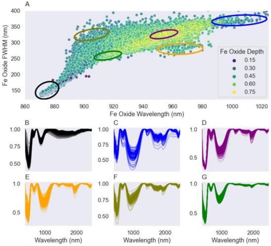
Figure 4.
The iron boomerang for the diamond core-only dataset (Core 1) with SWIR masking in place and selecting several key regions of interest (ROI) is shown in (A) and coloured by the Fe oxide depth. Figure (B–G) show the hull-corrected spectra. (B) is the left most portion of the iron boomerang comprised of hematite samples. (C) and located at the right hand most side of the iron boomerang are primarily vitreous goethite. (D) represents a region of mixed ochreous and vitreous goethite. (E) is generally purer ochreous goethite and does not exhibit the drop off observed in (C) and (D) from approximately 1300 nm. (F,G), respectively, show mixtures of hematite and goethite with at least two different goethite types (vitreous and ochreous, respectively).
The region labelled as mixed goethite (Figure 4D) in Figure 3 shows the difference in shape of the Fe absorption feature as compared to Figure 4C and the reduction in visible absorption features between 1500 and 1850 nm. Pure ochreous goethite does not exhibit the drop off observed at approximately 1300 nm (Figure 4C,D). Mixtures of hematite and vitreous goethite are observed (Figure 4F) whereas a mixture of hematite and ochreous goethite is shown in Figure 4G.
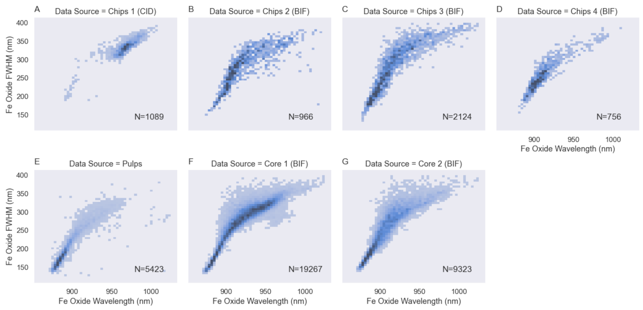
It is noted though that no seemingly strict separation, except for the leading edges of the iron boomerang beyond Fe oxide wavelengths of approximately 930 nm, is evident at this stage between ochreous and vitreous goethite. Figure 5 are the alteration-masked iron boomerang metrics for each of the individual data sources using a density plot for better visual comparison as noted in Figure 2B. Figure 5A is the Rocklea Dome CID RC chips set with 1089 samples, Figure 5B–D are for the Hamersley Basin BIF RC chips sets with 966, 2124, and 756 samples, respectively, Figure 5E is the Hamersley Basin BID pulp dataset comprised of 5423 samples and Figure 5F,G are the Hamersley Basin diamond core datasets with a total of 19,267 and 9323 samples, respectively.

Figure 5.
(A) is the Rocklea Dome CID RC chips set, (B–D) are for the Hamersley Basin BIF RC chip sets, (E) is the Hamersley Basin BIF pulp dataset and (F,G) are the Hamersley Basin diamond core datasets. (A) is primarily goethite and very little hematite. (D) is composed of a greater proportion of hematite with some hematite/goethite.
The separation of the individual datasets allows the general makeup of the individual datasets to be quickly and reasonably established. The CID dataset is found to be primarily composed of goethite and has very little hematite, resulting in overall high Fe oxide wavelength and Fe oxide FWHM (Figure 5A). For the BIF chips on the other hand, the trend is opposite as it is composed of a greater proportion of hematite with some hematite/goethite mixtures but far fewer goethite only samples, indicated by lower Fe oxide wavelength and Fe oxide FWHM values when compared to the CID. Figure 5B,C suggest a similar presence of hematite and hematite/goethite mixtures, with Figure 5C exhibiting a greater proportion of potential vitreous goethite, as evidenced by the samples with Fe oxide FWHM values above 360 nm and Fe oxide wavelengths beyond 1000 nm.
Figure 5F, G from the two core datasets are very similar in distribution and suggest a greater amount of mixing and similar assemblages, with Figure 5F showing a greater amount of long Fe oxide wavelength vitreous goethite samples. Note the greater amount of data (9000+ samples) in the diamond core iron boomerangs are primarily due to the far higher downhole sampling by the HyLoggerTM, with approximately 100 samples per metre.
Lastly, the iron boomerang applied to the Hamersley Basin BID pulp samples shows that the distribution would appear to show a heavy concentration of hematite and smaller amounts of hematite/goethite mixtures with the goethite being predominantly ochreous due to the Fe oxide FWHM being below 350 nm (Figure 5E). However, in this case, the distribution is affected by the nature of the sample media itself. Namely, the finer particle size of the pulps has the effect of removing or modifying several features associated with vitreous goethite. The SWIR dropoff metric is generally suppressed, and the Fe oxide wavelength shortened to smaller wavelengths. This has the effect of making vitreous goethite samples look very much like ochreous goethite samples when viewed spectrally. It is possible, but noted without proof, that the same effect is possibly present in both the RC chips and diamond core datasets where the samples have been effectively crushed or impacted by dust or fines coatings.
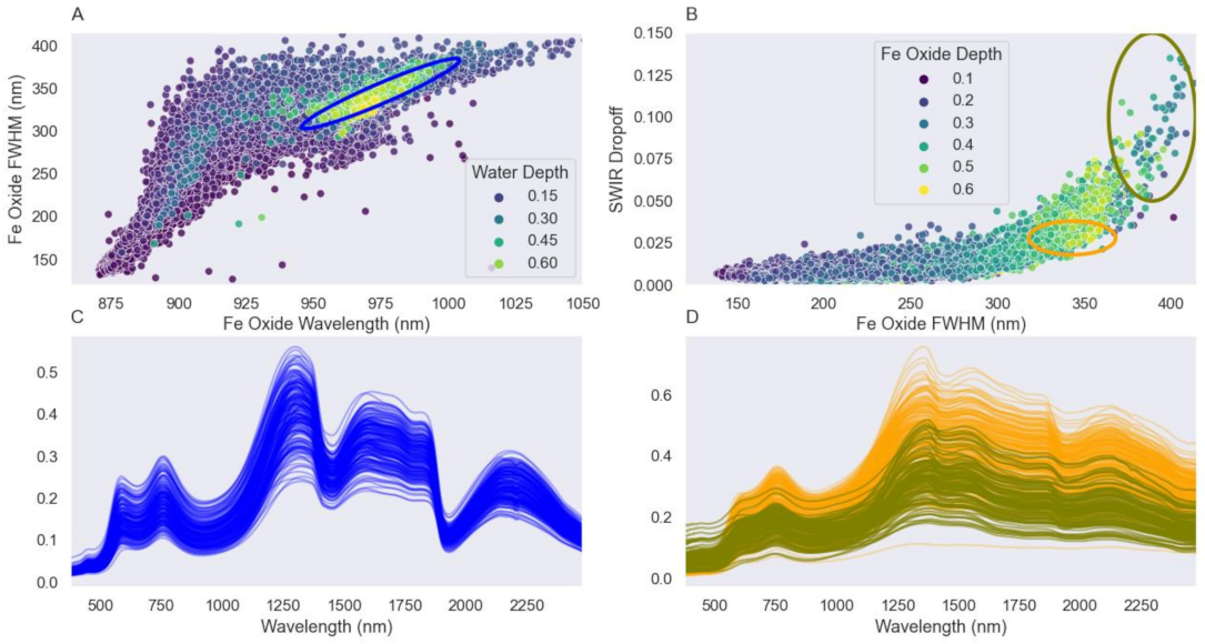
The use of the two other spectral metrics provides the extraction of additional information from the spectral datasets (Figure 6). The iron boomerang for the entire SWIR Masked datasets and coloured by the water depth metric reveals a large concentration of spectra with deep absorption features at approximately 1940 nm (Figure 6A), characteristic of the Rocklea Dome CID chips spectral dataset. These samples with a water depth metric greater than 0.6 and shown approximately circled in Figure 6A provide an additional separation of ochreous goethite types, and with potentially overlapping vitreous goethite, due to the large water absorption features.

Figure 6.
(A) is for the entire SWIR Masked datasets and coloured by the water depth. The spectra in (C) are extracted by selecting samples with a water depth metric greater than 0.6 and shown approximately circled in (A) and represent the Rocklea Dome CID spectra. (B) is the Fe oxide FWHM plotted against the SWIR dropoff for the Hamersley Basin the second diamond core dataset (Core 2, BIF). (B) is coloured by the Fe oxide depth for visualisation discrimination only but does show an increase in Fe oxide depth with increasing goethite and decreasing hematite. The olive is primarily vitreous goethite (D), while the orange region highlighted in (B) is representative of mixed vitreous and ochreous goethite.
As noted previously, the SWIR dropoff metric is an indicator of the presence of vitreous goethite increases as the Fe oxide FWHM also increases (Figure 6B). The olive region beyond an Fe oxide FWHM value of 360 nm is observed to have very low Fe oxide abundance values and is primarily vitreous goethite and it would run horizontally across the top of the iron boomerang (Figure 6D). The second region highlighted (orange in Figure 6B) corresponds to samples where the Fe oxide depth is greater than 0.6 and which contain more ochreous goethite. It is important to note that below the orange region, meaning plotted underneath the bright highlighted sample points, in Figure 6B are samples that can still contain vitreous goethite.
5. Discussion and Conclusions
Utilising a simple combination of two spectral metrics, namely the Fe oxide wavelength and the Fe oxide FWHM, it is demonstrated that a large collection of spectral samples from BIF, BID and CID of the Pilbara Province of Western Australia fall within a distinctive manifold. The manifold named the iron boomerang provides an overview of the dataset and offers a qualitative means of ascertaining the iron oxides paragenesis and when incorporated with other spectral metrics, the possibility to further subclass the goethite types.
It was shown that the distribution of the samples when examined in a density plot along the peripheries of the iron boomerang is lower than those within the core of the iron boomerang probably because of the samples mostly occurring in BID.
If the dataset contains unmixed hematite and vitreous goethite, then two spectral endmembers can be located at either end of the iron boomerang. Samples comprised of the shortest Fe oxide wavelengths and the smallest Fe oxide FWHM values are comprised of hematite while those at approximately 1050 nm and with an Fe oxide FWHM value greater than 370 nm are observed to be vitreous goethite. Additionally, samples along the top edge of the iron boomerang and above a Fe oxide FWHM of 360 nm, and with a combined low SWIR dropoff metric value, are predominantly vitreous goethite. The selection of potential ochreous goethite samples can be achieved by selecting samples that have Fe oxide wavelengths greater than 930 nm and lie along the bottom edge of the iron boomerang.
It is tempting to infer that a traverse along any of the iron boomerangs outer edges might be representative of a two-member spectral mixture, namely hematite and goethite. Further work with known mixtures of hematite and goethite is required to evaluate the potential mixing pathways within the iron boomerang. Additionally, even though previous studies have established a hematite–goethite ratio, it would be beneficial in any future work to assess if the ratios are affected by the type of hematite and goethite used. This could be done when assessing the potential mixing pathways. The ability to identify at least three mineral types, hematite as well as vitreous and ochreous goethite, should allow a selection of representative samples to test the mixing pathways and the effects that they may have on the iron boomerang and the hematite–goethite ratio.
Samples that contain spectral absorptions due to the presence of weathering minerals were found to have an impact on the overall distribution of the iron boomerang. The presence of kaolinite was observed to induce a reduction in the calculated Fe oxide FWHM value. Weathered samples are easily masked out and do not present a major issue. In this study, the number of samples that were impacted by the presence of alteration minerals was approximately 33%.
It was demonstrated that the iron boomerang, when examined as a per dataset collection, allows an overview of each dataset relative to each other and thus provides a direct comparison of the datasets. However, it is worth noting the impact of crushing and reducing the particle size on the individual spectral samples. The iron boomerang yielded from the Hamersley Basin pulp samples is known to contain hematite, vitreous goethite and ochreous goethite. However, the decreased particle size has seemingly reduced the range of Fe oxide wavelengths and Fe oxide FWHM values that might be expected when the other datasets are examined. It is noted that, in this case, the features that are indicative of vitreous goethite, such as larger SWIR dropoff values and larger Fe oxide wavelength and Fe oxide FWHM values, have been suppressed and give the overall impression of the spectral samples being more ochreous in spectral appearance. It may be the case that if the iron boomerang is used in conjunction with pulps, it will benefit from two spectral scans—the first would be prior to crushing and the second after crushing, where the effect of the different sample particle sizes can be related back via the sample identity. Future work will also seek to ascertain the effect of the iron boomerang parameters as a function of particle size. Additionally, other future work will seek to evaluate the iron boomerang in relation to the geochemistry of the samples to ascertain if the trends within the iron boomerang are attributable to the mineral chemistry or a product driven by the mixture and/or hardness of the sample.
Author Contributions
Conceptualization, A.R.; methodology, A.R.; software, A.R.; validation, A.R., E.R., I.L. and C.L.; formal analysis, A.R., E.R., I.L. and C.L.; writing—original draft preparation, A.R.; writing—review and editing, A.R., E.R., I.L. and C.L. All authors have read and agreed to the published version of the manuscript.
Funding
This work was funded as part of Minerals Research Institute of Western Australia (MRIWA) project 557.
Institutional Review Board Statement
Not applicable.
Informed Consent Statement
Not applicable.
Data Availability Statement
The data used within this study are subject to proprietary constraints and are not publicly available. However, the Rocklea Dome dataset is publicly available (https://data.csiro.au/collection/csiro:44783v1).
Acknowledgments
The authors would like to acknowledge the following for their support: BHP Iron Ore, Bureau Veritas, CSIRO Mineral Resources, FMGL, MRIWA, Rio Tinto Iron Ore and Roy Hill.
Conflicts of Interest
The authors declare no conflict of interest.
References
- Haest, M.; Cudahy, T.; Laukamp, C.; Gregory, S. Quantitative mineralogy from infrared spectroscopic data. I. Validation of mineral abundance and composition scripts at the rocklea channel iron deposit in Western Australia. Econ. Geol. 2012, 107, 209–228. [Google Scholar] [CrossRef]
- Ramanaidou, E.R.; Wells, M.A. Hyperspectral Imaging of Iron Ores. In Proceedings of the Proceedings of the 10th International Congress for Applied Mineralogy (ICAM); Springer: Berlin, Germany, 2012; pp. 575–580. [Google Scholar]
- Ramanaidou, E.R.; Schodlok, M. Hyperspectral Mapping of Bif and Iron Ores. In Proceedings of the AGU Fall Meeting Abstracts; AGU: San Francisco, CA, USA, 2012; Volume 2012, p. NS23A-1630. [Google Scholar]
- Fouedjio, F.; Hill, E.J.; Laukamp, C. Geostatistical clustering as an aid for ore body domaining: Case study at the rocklea dome channel iron ore deposit, Western Australia. Appl. Earth Sci. 2018, 127, 15–29. [Google Scholar] [CrossRef]
- Cudahy, T.J.; Ramanaidou, E.R. Measurement of the hematite: Goethite ratio using field visible and near-infrared reflectance spectrometry in channel iron deposits, Western Australia. Aust. J. Earth Sci. 1997, 44, 411–420. [Google Scholar] [CrossRef]
- Haest, M.; Cudahy, T.; Laukamp, C.; Gregory, S. Quantitative mineralogy from infrared spectroscopic data. II. Three-dimensional mineralogical characterization of the rocklea channel iron deposit, Western Australia. Econ. Geol. 2012, 107, 229–249. [Google Scholar] [CrossRef]
- Ramanaidou, E.; Wells, M.; Lau, I.; Laukamp, C. 6—Characterization of Iron Ore by Visible and Infrared Reflectance and Raman Spectroscopies. In Iron Ore; Lu, L., Ed.; Woodhead Publishing: Sawston, UK, 2015; pp. 191–228. ISBN 978-1-78242-156-6. [Google Scholar]
- Cudahy, T.; Jones, M.; Thomas, M.; Laukamp, C.; Caccetta, M.; Hewson, R.; Verrall, M.; Hacket, A.; Rodger, A. Mineral Mapping Queensland: Iron Oxide Copper Gold (IOCG) Mineral System Case History, Starra, Mount Isa Inlier; Australasian Institute of Mining and Metallurgy: Gold Coast, Queensland, Australia, 2008; pp. 153–160. [Google Scholar]
- Rodger, A.; Laukamp, C.; Haest, M.; Cudahy, T. A simple quadratic method of absorption feature wavelength estimation in continuum removed spectra. Remote Sens. Environ. 2012, 118, 273–283. [Google Scholar] [CrossRef]
- Laukamp, C.; Termin, K.A.; Pejcic, B.; Haest, M.; Cudahy, T. Vibrational spectroscopy of calcic amphiboles—Applications for exploration and mining. Eur. J. Mineral. 2012, 24, 863–878. [Google Scholar] [CrossRef]
- Duuring, P.; Laukamp, C. Mapping Iron Ore Alteration Patterns in Banded Iron-Formation Using Hyperspectral Data: Beebyn Deposit, Pilbara Craton, Western Australia; Geological Survey of Western Australia: Perth, Australia, 2016. [Google Scholar]
- Rodger, A.; Fabris, A.; Laukamp, C. Feature extraction and clustering of hyperspectral drill core measurements to assess potential lithological and alteration boundaries. Minerals 2021, 11, 136. [Google Scholar] [CrossRef]
- Laukamp, C.; Rodger, A.; le Gras, M.; Lampinen, H.; Lau, I.C.; Pejcic, B.; Stromberg, J.; Francis, N.; Ramanaidou, E. Mineral physicochemistry underlying feature-based extraction of mineral abundance and composition from shortwave, mid and thermal infrared reflectance spectra. Minerals 2021, 11, 347. [Google Scholar] [CrossRef]
- Murphy, R.J.; Monteiro, S.T. Mapping the distribution of ferric iron minerals on a vertical mine face using derivative analysis of hyperspectral imagery (430–970 Nm). ISPRS J. Photogramm. Remote Sens. 2013, 75, 29–39. [Google Scholar] [CrossRef]
- Magendran, T.; Sanjeevi, S. Hyperion image analysis and linear spectral unmixing to evaluate the grades of iron ores in parts of Noamundi, Eastern India. Int. J. Appl. Earth Obs. Geoinf. 2014, 26, 413–426. [Google Scholar] [CrossRef]
- Hecker, C.; van der Meijde, M.; van der Meer, F.D. Thermal infrared spectroscopy on feldspars—Successes, limitations and their implications for remote sensing. Earth-Sci. Rev. 2010, 103, 60–70. [Google Scholar] [CrossRef]
- Mauger, A.J.; Ehrig, K.; Kontonikas-Charos, A.; Ciobanu, C.L.; Cook, N.J.; Kamenetsky, V.S. Alteration at the Olympic dam IOCG–U deposit: Insights into distal to proximal feldspar and phyllosilicate chemistry from infrared reflectance spectroscopy. Aust. J. Earth Sci. 2016, 63, 959–972. [Google Scholar] [CrossRef]
- Ramanaidou, E.R.; Wells, M.A. 13.13—Sedimentary Hosted Iron Ores. In Treatise on Geochemistry, 2nd ed.; Holland, H.D., Turekian, K.K., Eds.; Elsevier: Oxford, UK, 2014; pp. 313–355. ISBN 978-0-08-098300-4. [Google Scholar]
- Manuel, J.R.; Clout, J.M.F. Goethite classification, distribution and properties with reference to Australian iron deposits. Proc. Iron Ore 2017, 567–574. [Google Scholar]
- Huntington, J.; Mauger, A.; Skirrow, R.; Bastrakov, E.; Connor, P.; Mason, P.; Keeling, J.; Coward, D.; Berman, M.; Phillips, R.; et al. Automated mineralogical core logging at emmie bluff iron oxide-copper-gold prospect. MESA J. 2006, 41, 38–44. [Google Scholar]
- Huntington, J.; Whitbourn, L.; Mason, P.; Berman, M.; Schodlok, M.C. HyLogging—Voluminous Industrial-Scale Reflectance Spectroscopy of the Earth’s Subsurface. In Proceedings of the Proceedings of ASD and IEEE GRS; Art, Science and Applications of Reflectance Spectroscopy Symposium, Boulder, CO, USA, 23–25 February 2010; Volume 2, p. 14. [Google Scholar]
- Schodlok, M.C.; Whitbourn, L.; Huntington, J.; Mason, P.; Green, A.; Berman, M.; Coward, D.; Connor, P.; Wright, W.; Jolivet, M. HyLogger-3, a visible to shortwave and thermal infrared reflectance spectrometer system for drill core logging: Functional description. Aust. J. Earth Sci. 2016, 63, 929–940. [Google Scholar]
- Fonteneau, L.C.; Martini, B.; Elsenheimer, D. Hyperspectral imaging of sedimentary iron ores–beyond borders. ASEG Ext. Abstr. 2019, 2019. [Google Scholar] [CrossRef] [Green Version]
- Gilroy, P.; Haest, M.; Taylor, S.; Hacket, A.; Lock, S. Development of an Empirical Geo-Metallurgical Model That Unlocks Value of the Mineral Resources at Yandi Mine; McGill University: Montreal, QC, Canada, 2018. [Google Scholar]
- Murphy, R.; Schneider, S.; Monteiro, S. Consistency of measurements of wavelength position from hyperspectral imagery: Use of the ferric iron crystal field absorption at 900 Nm as an indicator of mineralogy. IEEE Trans. Geosci. Remote Sens. 2014, 52, 2843–2857. [Google Scholar] [CrossRef]
- Haest, M.; Cudahy, T.; Laukamp, C.; Ramanaidou, E.; Gregory, S.; Stark, J.C.; Podmore, D. Characterisation of Bedded and Channel Iron Ore Deposits Using CSIRO’s Hyloggingtm Systems. In Proceedings of the Iron Ore 2011 Meeting Growing Demand, Perth, Australia, 10–13 July 2011. [Google Scholar]
- Thompson, A.J.; Hauff, P.L.; Robitaille, A.J. Alteration mapping in exploration: Application of short-wave infrared (SWIR) spectroscopy. SEG Discov. 1999, 39. [Google Scholar] [CrossRef]
- Berman, M.; Bischof, L.; Huntington, J. Algorithms and Software for the Automated Identification of Minerals Using Field Spectra or Hyperspectral Imagery. In Proceedings of the Proceedings of the 13th International Conference on Applied Geologic Remote Sensing, Vancouver; Environmental Research Institute of Michigan: Ann Arbor, MI, USA, 1999; Volume 1, pp. 222–232. [Google Scholar]
- Mauger, A.J.; Herbert, H.K.; Baker, A.H. AuScope national virtual core library–SA node. ASEG Ext. Abstr. 2010, 2010. [Google Scholar] [CrossRef] [Green Version]
- Sunshine, J.M.; Pieters, C.M.; Pratt, S.F. Deconvolution of mineral absorption bands: An improved approach. J. Geophys. Res. Solid Earth 1990, 95, 6955–6966. [Google Scholar] [CrossRef] [Green Version]
- Wells, M.A.; Ramanaidou, E.R. Clay quantification of channel iron deposits (CID), Pilbara, Western Australia. Proc. Iron Ore 2007, 6, 203–207. [Google Scholar]
- Laukamp, C.; Haest, M.; Cudahy, T. The rocklea dome 3D mineral mapping test data set. Earth Syst. Sci. Data 2021, 13, 1371–1383. [Google Scholar] [CrossRef]
- Townsend, T.E. Discrimination of iron alteration minerals in visible and near-infrared reflectance data. J. Geophys. Res. Solid Earth 1987, 92, 1441–1454. [Google Scholar] [CrossRef]
- Morris, R.V.; Lauer, H.V., Jr.; Lawson, C.A.; Gibson, E.K., Jr.; Nace, G.A.; Stewart, C. Spectral and other physicochemical properties of submicron powders of hematite (α-Fe2O3), maghemite (γ-Fe2O3), magnetite (Fe3O4), goethite (α-FeOOH), and lepidocrocite (γ-FeOOH). J. Geophys. Res. Solid Earth 1985, 90, 3126–3144. [Google Scholar] [CrossRef] [PubMed]
- Buckingham, W.F.; Sommer, S.E. Mineralogical characterization of rock surfaces formed by hydrothermal alteration and weathering; application to remote sensing. Econ. Geol. 1983, 78, 664–674. [Google Scholar] [CrossRef]
- Frost, R.L.; Johansson, U. Combination bands in the infrared spectroscopy of kaolins—A DRIFT spectroscopic study. Clays Clay Miner. 1998, 46, 466–477. [Google Scholar] [CrossRef]
- Kokaly, R.F.; Clark, R.N.; Swayze, G.A.; Livo, K.E.; Hoefen, T.M.; Pearson, N.C.; Wise, R.A.; Benzel, W.M.; Lowers, H.A.; Driscoll, R.L.; et al. USGS Spectral Library Version 7; Data Series; U.S. Geological Survey: Reston, VA, USA, 2017; Volume 1035, p. 68.


Publisher’s Note: MDPI stays neutral with regard to jurisdictional claims in published maps and institutional affiliations. |
© 2022 by the authors. Licensee MDPI, Basel, Switzerland. This article is an open access article distributed under the terms and conditions of the Creative Commons Attribution (CC BY) license (https://creativecommons.org/licenses/by/4.0/).