1. Introduction
Production lines often encounter downtime, either planned or unplanned. Though planned downtime affects the Overall Equipment Efficiency (OEE), it can be reduced by an optimized usage plan. In contrast, unplanned downtime, as the name suggests, is not planned beforehand and is typically due to the component failure, tool breakage or other technical stoppage. It is difficult to foresee some of these failures and plan the maintenance tasks accordingly. Predictive or condition-based maintenance is a solution that can be employed in manufacturing industries to reduce this unplanned downtime. Predictive maintenance methods, by predicting the condition of a machine or a component, allow dynamic and convenient maintenance scheduling, thus making it an adequate option for modern manufacturing industries [
1]. Predictive maintenance, from the authors’ perspective, is accomplished in three important steps: (1) monitor a machine, (2) predict if something is anomalous and the machine is prone to failure and (3) make sure it is maintained without causing any disturbance to the planned production. In situ deployed sensors take care of the monitoring aspect, whereas fault prediction and maintenance are traditionally manual procedures. This intermediate task of predicting the early faults whilst monitoring the machines has been researched for a long time [
2]. Importantly, there are two types of fault diagnosis methods to monitor machines or machine components, model-based and data-driven. Though very commonly used, the mathematical model of a fault diagnosis system designed using a model-based method cannot take into account all the noises or subtle variations that a system is exposed to [
3]. Hence, depicting an accurate machine model or open-source availability of such models is unfeasible, whereas using an inaccurate model may lead to poor fault diagnostic performance in practice. Unlike the model-based approaches, data-driven methods utilize the collected in-process data. These data are analyzed, and the acquired knowledge is used to build a fault diagnosis model. This allows a user to apply diagnostics even when there are no available mathematical models of a particular machine. It also includes noise and a certain degree of variations into the diagnostic model. This noise inclusion into the diagnostic model is simple, with data-driven modeling compared to the model-based method [
3], thus making it a more desirable solution for fault diagnosis.
Recently, data-driven methods have been performing exceptionally well in predictive fault diagnosis [
4,
5,
6,
7]. One of the main reasons for the increased performance of data-driven models over model-based methods is the availability of open source datasets. Looking into the state of the art for predictive maintenance in the manufacturing industry, most data-driven approaches focus on finding bearing faults, as these are the most predominant source of machine downtime [
8]. There is a lot of research that shows very good classification results for bearing fault detection on the standard datasets that exist for vibration-based rolling element faults. Toma et al. show how a 1D Convolutional Neural Network (CNN) can be used on time domain data to accurately predict a bearing fault [
9]. Moreover, by reshaping the time domain vibration data into a 2D array, i.e., into an image-style input, the two dimensional convolutional operations were used for feature extraction [
10,
11]. This study further presented the improved accuracy of the 2D CNNs for both normal and noisy data using the time domain data as input. Unlike the above, other works have shown the effectiveness of time-frequency transformed features for bearing fault detection [
12]. In their study, only a few selective features of Empirical Mode Decomposition were used along with certain Machine Learning algorithms for effective classification of bearing faults. In [
13], the authors derived an entrogram from the time series data using Frequency Slice Wavelet Transform, which they analyzed to see if the bearing faults can be distinguished from the normal working condition. A state of the art (SOTA) survey on various methodologies used for bearing fault diagnosis is detailed in [
14]. As can be observed from this article, there are numerous ways of detecting bearing faults. The results show that bearing fault classification is effective when sufficient data from different conditions is available.
However, variability in the machine operating conditions poses a practical problem for condition-based monitoring. Furthermore, it is impractical to collect the data for all these variabilities (e.g., settings under which a machine operates, such as axial load, radial load, rotation speed, etc.). As we know, general features from the observations
of two different machine conditions do not always fall in a similar distribution. For example, data collected in a lab setting can be different to the data acquired from a similar setup in the field. Generic algorithms that are trained with the data from labs are then prone to transfer errors when used to infer the results from data measured in the field [
15]. Similarly, the variation in the data can be caused by many parameters such as operating conditions, sensor displacement, variation in the sensor, etc., and it is currently a challenge to develop a model that is robust to these variations.
In an attempt to generalize the classification across conditions, researchers have proposed several algorithms that transfer the learning from one condition to another [
15], where the class distribution from one condition is known (source domain) and some information of another condition (target domain) to which the class information will be fitted and matched. To tackle the problem of needing data from all possible conditions, unlike the existing methods, we propose a new approach based on latent features of Auto-Encoders and nearest neighbor algorithms. This novel methodology considers any one condition’s data and performs a robust classification across other conditions. For different open-source datasets, we then compared our method to the best performing source only methods and domain adaptation methods from the SOTA. This work is structured as follows.
Section 2 gives the detailed problem description, which is followed up by
Section 3, where we discuss some preliminaries necessary for understanding this work. The proposed methodology is then described in
Section 4, succeeded by Experimental Setup, Results, and Conclusions in
Section 5,
Section 6 and
Section 7, respectively.
2. Problem Description and Related Work
Before describing the problem, some notations and definitions regarding the problem are introduced.
Transfer Learning: The process of learning the information from the data of one condition and transferring the knowledge to a new condition.
Source Domain: The condition of the machine from which the data are collected and is used to train the fault diagnosis model.
Target Domain: The condition of the machine from which the data are collected and is used to test the knowledge transfer.
Transfer of class knowledge in Transfer Learning (TL) tasks can be classified into two methods. This is based on what is available during the training process:
Robust Learning: Refers to how to appropriately predict class label of the jth observation of the target domain when there is an available set of observations from the source domain
Domain adaptation: In some cases, a few observations from the target domain are also available, and the model is adapted to the target domain. This is called domain adaptation.
Here, is the sample set of the ith observation from the source domain, and is the corresponding label of that observation. In addition, and stand for the sample set and corresponding label in the target domain, respectively.
While applying this to an industrial machine, the domains represent different conditions. There are various TL tasks from the literature that learn the distribution of the
and tries to adapt to the distribution of
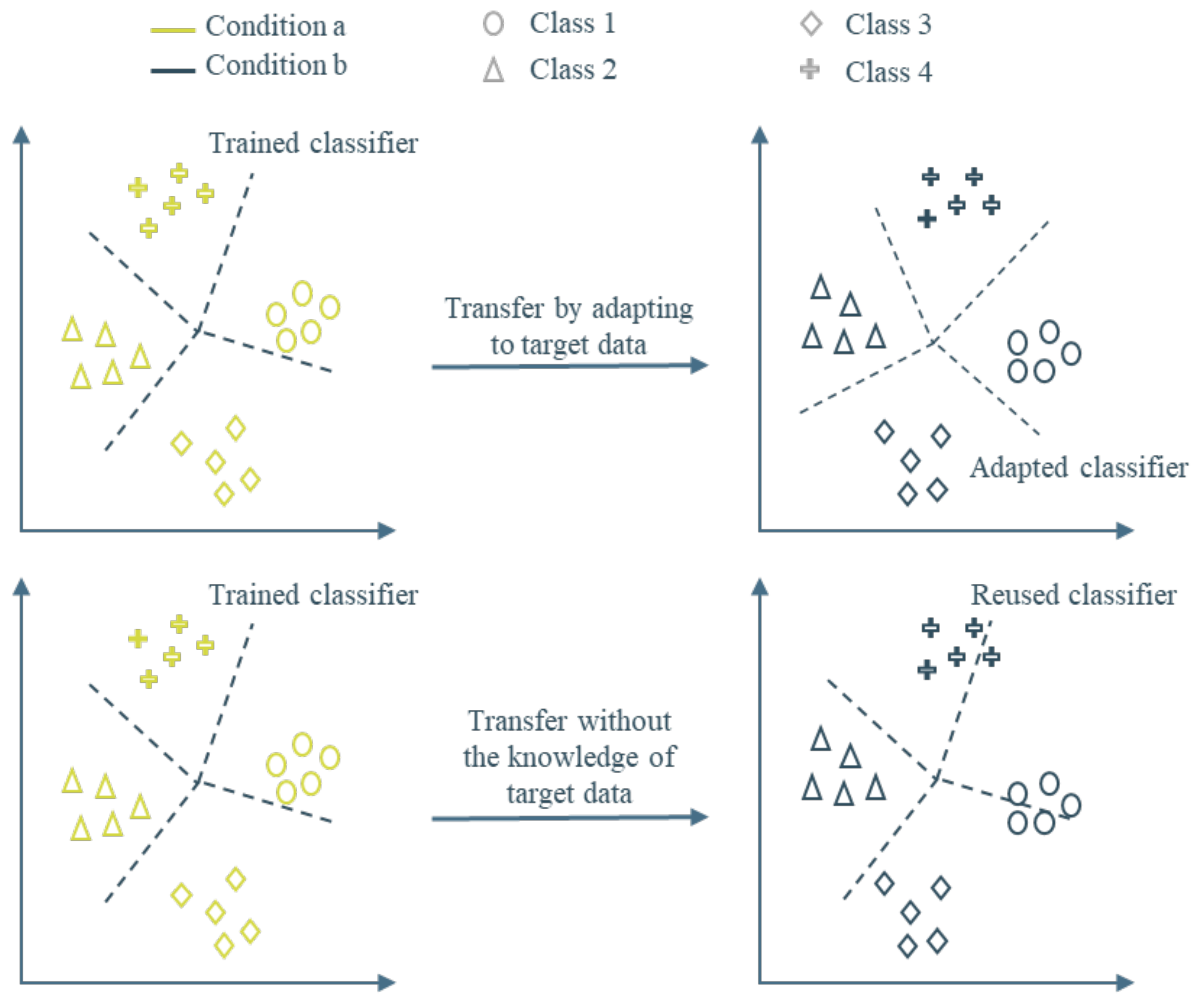
. As represented in
Figure 1, some methods train using information from the target domain, which can be considered as Domain Adaptation methods, and some do not; these can be considered as Robust Learners. The problem considered in this work is robust learning as, most of the time, the target domain data are scarce and infeasible to collect.
From the investigated literature, there are many transfer learning methodologies between machine conditions which have achieved high accuracies. The majority of these methods are domain-adaptation-based transfers of learning. The following are the state-of-the-art articles in the domain adaptation for bearing fault diagnosis. Wang et al. [
8] proposed one such domain adaptation method named MDIAN. In [
8], the authors use a modified ResNet-50 structure to extract multiple scale features and to try to reduce the conditional maximum mean discrepancy using the so extracted features of source and target domain observations. As reported in their work, MDIAN outperforms several SOTA approaches, such as Convolutional Neural Network (CNN) and CNN + Maximum Mean Discrepancy, for various transfer learning tasks of fault diagnosis. In another domain adaptation work, Li et al. [
16] proposed a methodology where features from vibration data are extracted using a Convolutional Neural Network. Along with the general prediction loss of the source domain data, this CNN parallelly trains to minimize the central moment discrepancy between the source and target distributions. They have achieved great transfer learning accuracies across conditions for various datasets. To the knowledge of the authors, it has been the best performing algorithm yet for the task of transfer learning given some target domain data. Furthermore, Li et al. [
16] also described their implementation of several algorithms such as CNN-NAP (Nuisance Attribute Projection) [
17] and MCNN (Multitask Convolutional Neural Network) [
18] from the literature for transfer learning of machine faults. The uniqueness of these implementations (CNN-NAP, MCNN) is that they use a source-only dataset to train the classifier, similar to the consideration in this work. Though they are the only other robust learning methodologies that are comparable with this work, they are not much better than a simple Convolutional Neural Network when considered for inter-conditional classification [
18]. Thus, these above-mentioned methodologies from the literature, indiscriminative of domain adaptation or robust learner, will be further used to compare our proposal.
Contributions of this work are:
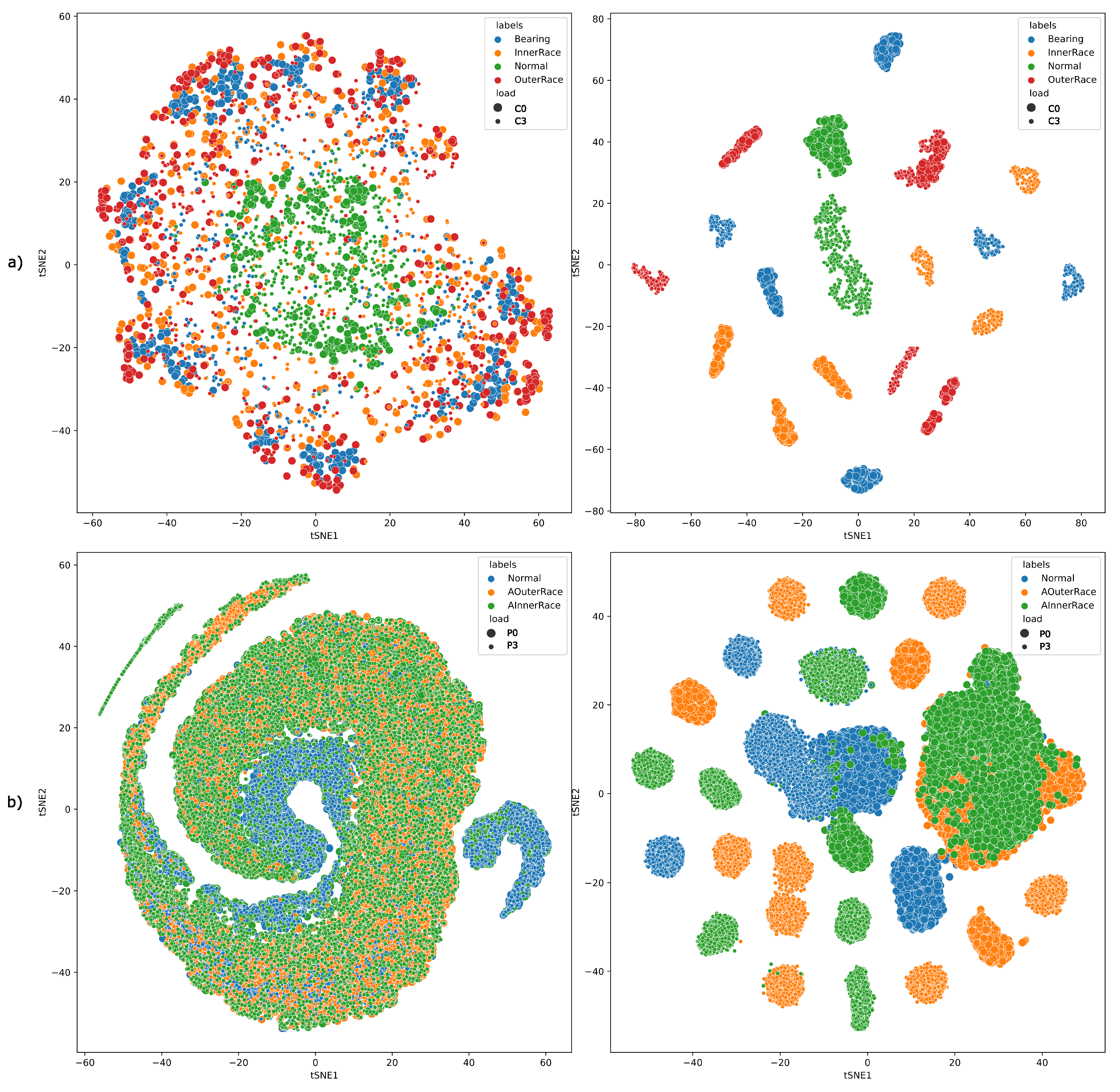
The empirical evaluation of Auto-Encoder latent features as robust features across conditions was performed. It was systematically performed using various transfer tasks of two widely used open source bearing fault datasets.
A simple methodology combining latent values of the Auto-Encoder and their proximity in the latent space is proposed for robust inter-conditional bearing fault diagnosis, given only the source domain data for training.
The results of the proposed method are presented and compared with the results of the other state-of-the-art methods.
Furthermore, in this work, the transfer learning experiments are considered to be homogeneous and use source-only datasets for training (robust learner). Homogeneous here refers to the classes being consistent across both source and target domain, whereas a source-only dataset means the trained algorithm does not consider any information of the target domain data. These constraints on the experiments are based on the practical requirement for industries, where gathering data is a difficult task. Thus, to tackle the challenge efficiently, a robust learner is proposed in this work.
5. Experimental Validation
To prove the effectiveness of the proposed methodology for robust transfer learning across conditions, we developed an experimental setup. There are important aspects of this setup, considered datasets, transfer learning tasks and chosen methods from the state-of-the-art to compare the results against.
5.1. Computational Unit and Training Time
The experiments have been performed on a DELL precision 5530. The configuration of the computational unit used for further experiments is as follows: 32GB RAM, 6 2.6GHz processors and an NVIDIA Quadro P2000 Graphical Programming Unit. The experimental scripts are written in Python 3.7.8.
The loss function used for training the MLCAE is the Mean Squared Error loss, and the stochastic optimizer used was Adam. The training times differ from task to task. For each transfer task, it takes approximately about 30 s to train with CWRU data and 400 s with PU data. Inference times are quite fast and were thus not measured.
5.2. Compared Methods
As discussed in the related work section, state-of-the-art methods mentioned in
Table 2 were chosen to compare the results. Two of the compared methodologies, Support Vector Machine (SVM) and Convolutional Neural Network (CNN), are source-only methods similar to our proposal, whereas CNN-MMD (CNN- Maximum Mean Discrepancy), MDDAN, MDIAN and CMD (Central Mean Discrepancy) use some information from the target domain for the transfer tasks. Nevertheless, we made the comparisons to show the effectiveness of the proposed method against state-of-the-art domain adaptation methods.
5.3. Evaluation Metric, Training and Testing Process
The evaluation of the proposed method is performed using Accuracy as a metric. Accuracy here is sufficient, as the considered cases are balanced across different labels.
True Positives (TP) and True Negatives (TN) together form the total number of samples that are predicted properly.
5.4. Architecture of the Auto-Encoder
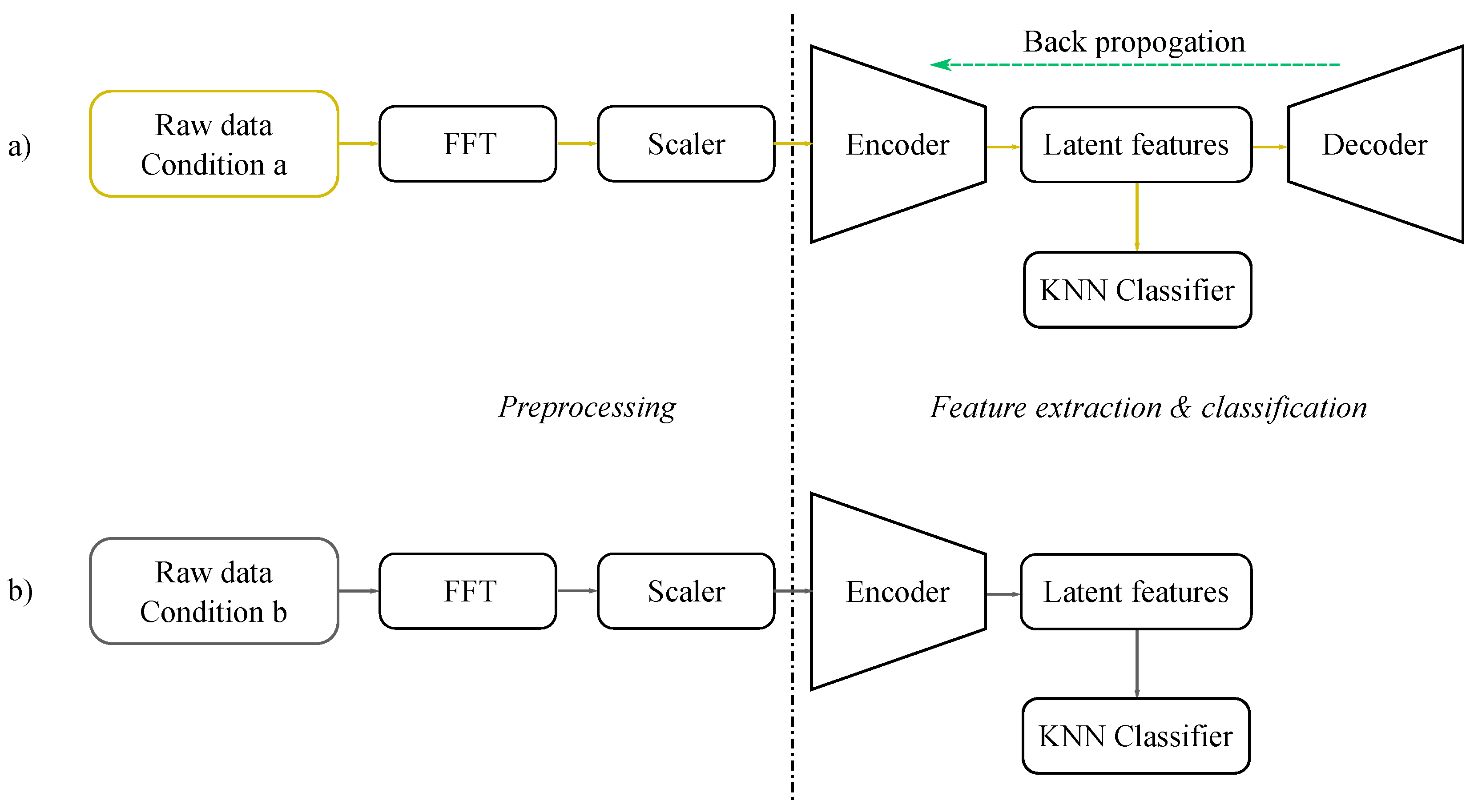
Upon investigating the classification results of our methodology on the validation data (a part of the training dataset), we understood that the frequency features as inputs to the MLCAE are better at segregating appropriate classes than the raw data. Thus, the inputs to the MLCAE in further experiments will be the magnitude of the positive spectrum of the FFT data. In the case of the CWRU dataset, each observation consisted of 1024 sample points so that it approximately fits information of two rotations of the motor spindle. This means that considering only the positive spectrum of the FFT data will lead to an input size of (512,1) for the CWRU dataset. Similarly, to approximately fit the information of two spindle rotations, the samples in each observation for the Paderborn data were chosen as 4096. Thus, the input size of the architecture used for Paderborn will be of size (2048,1). Some of the parameters used in architectures for CWRU and Paderborn are similar, whereas some are not. Details of these parameters are also mentioned in
Table 3.
Such AE-based extractors are trained with the FFT data of each condition. During the process of training, it considers the loss of reconstruction and tries to minimize this loss while optimizing the whole network. Once the stop criteria (non-reducing loss or suggested epochs) are met, the training algorithm stops, and the encoder part of the so-trained AE is considered for further usage. When an observation from a different condition is inferred using this encoder, it produces a reduced number of features (values from the latent dimension), which will then be used as inputs to train the classifier. Numerically, the MLCAE (Multi Layer Convolutional AE) will train and bring sizes of (512,1) of CWRU and (2048,1) of Paderborn to (20,1) latent dimensions, which will then be used by the KNN classifier for further classification.
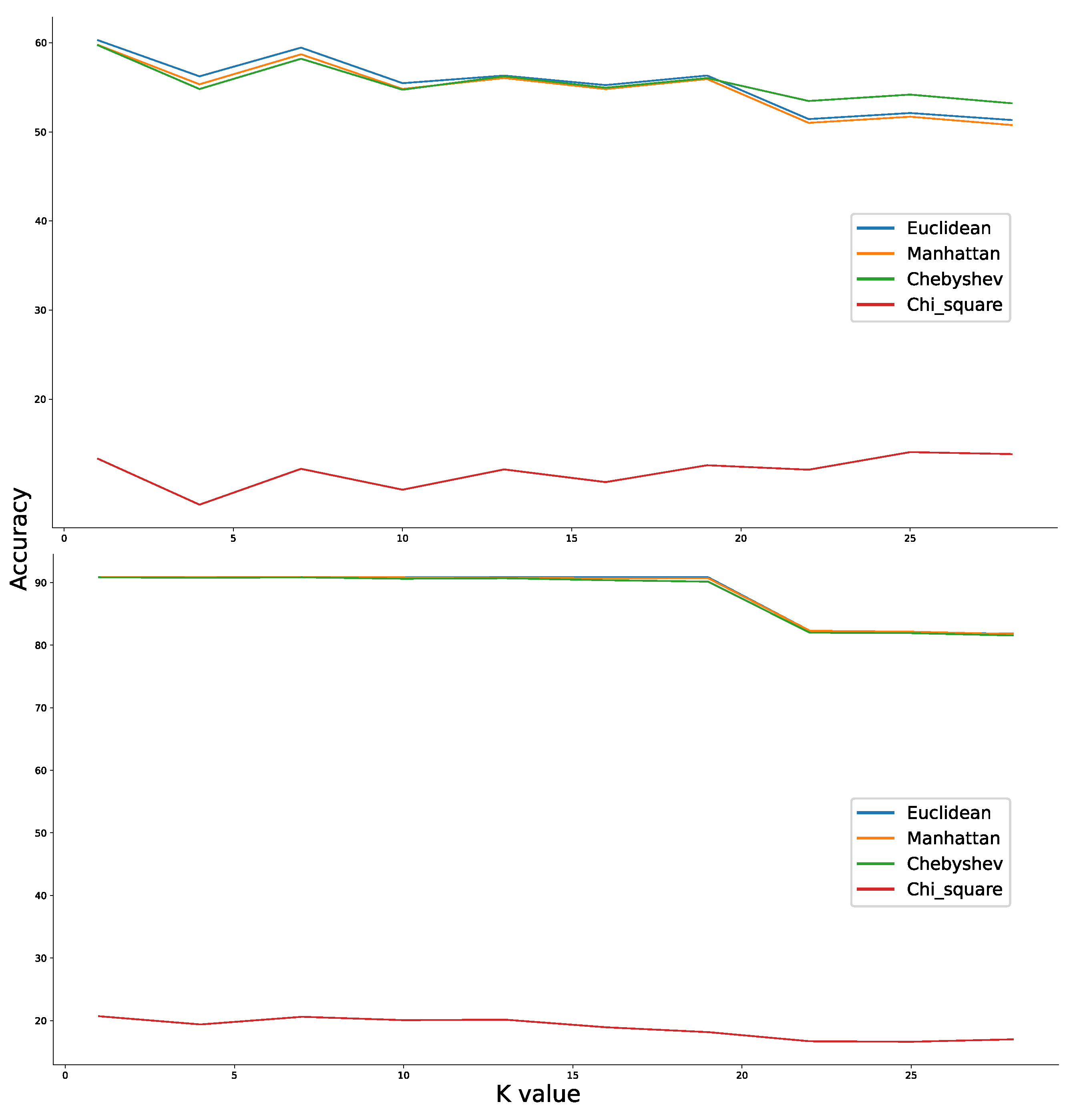
We also discussed in the previous section that the choice of K value for the KNN may fall anywhere between 1 and 15. Upon further investigation for random transfer tasks, the classification results across conditions were inconsistent when the K values are small and was showing degraded performance across conditions when the value is high. The exact nearest number of observations to consider for predicting a new sample in case of both the datasets was thus found to be optimal at k = 5.
The trained classifier from one condition was then tested against other conditions, and the experimental results for various transfer tasks were discussed accordingly. The training and testing process adopted in this article is as described in Algorithm 1.
| Algorithm 1 Pseudo algorithm used for training and testing various transfer tasks of CWRU and PU datasets. |
- 1:
Training Input: Labeled source domain data - 2:
Training Output: Min-Max Scaler (), Auto-Encoder Network (encoder and decoder ) and K-Nearest Neighbours classifier () - 3:
Testing Input: Labeled target domain data and , and - 4:
Testing Output: Predicted labels of target domain data - 5:
Begin: - 6:
for each value of i in range of n: - 7:
Train and transform with as shown by Equation (3) - 8:
for (m epochs or stopping criteria met): - 9:
Optimize with MSE as shown in (1) - 10:
end for - 11:
Compute latent features of using Equation (2) - 12:
Train with and - 13:
for each value of k in range of n and : - 14:
Transform with - 15:
Compute latent features of with - 16:
Predict with and - 17:
Compute accuracy of prediction with and - 18:
end for - 19:
end for
|
As an important note, the normalisation part of our pre-processing step has two separate methods for the train and test datasets. Considering the goal of using a source-only dataset for algorithm training, the test dataset (target domain data) will not be used during the training process. The same scaler that is used to fit against and transform the training data will be used to transform the test data. In this way, we make sure that no information of the target domain is used during training.
7. Conclusions
In the context of condition-based monitoring, the collection of data from different conditions/different machine settings is a difficult task and is sometimes even impossible. Ideally, it is efficient to perform transfer of learning from one condition to another. We proposed a source-only methodology to effectively transfer class learning between conditions of a machine for bearing fault detection. We implemented and compared the performance with various state-of-the-art transfer learning methods, both source-only methods (SVM and CNN) and domain adaptation methods (CNN-MMD, MDDAN, MDIAN and CMD) for a set of tasks. From the results, the following can be concluded:
- (1)
The proposed method performs more robust classification compared to other transfer learning methods. For many inter-conditional transfer tasks, the MLCAE-KNN source-only method performs as good or better than the other domain adaptation methods that consider certain information from the target domain.
- (2)
Though the proposed methodology is robust, for some transfer tasks, it has a certain deviation in the accuracies across different runs (up to 6% for certain tasks of the Paderborn dataset, as presented in
Table 5).
- (3)
In our observation with the experiments of MLCAE-KNN, training a classifier using data from higher parameter settings (rotational speed, radial load, etc.) and transferring the learning onto lower settings provides better a transfer of class learning compared to the other way around.
As for how and what effects a transfer learning task has across conditions is still a preliminary hypothesis, further investigation is needed. To further validate our proposal and the preliminary hypothesis, as a future work we will investigate transfer of class learning tasks by considering other datasets for a similar application. In addition, as discussed in the proposed methodology, one of the criteria is to keep the AE structure simple. This is due to its intended use on resource-constrained embedded devices. Thus, our future work also extends to investigating the practicalities of inferring MLCAE-KNN on an embedded device.


 ,
, 


