
Sub-Harmonic Response Analysis of Nonlinear Dynamic Behaviors Induced by Piecewise-Type Nonlinearities in a Torsional Vibratory System


Abstract
:1. Introduction
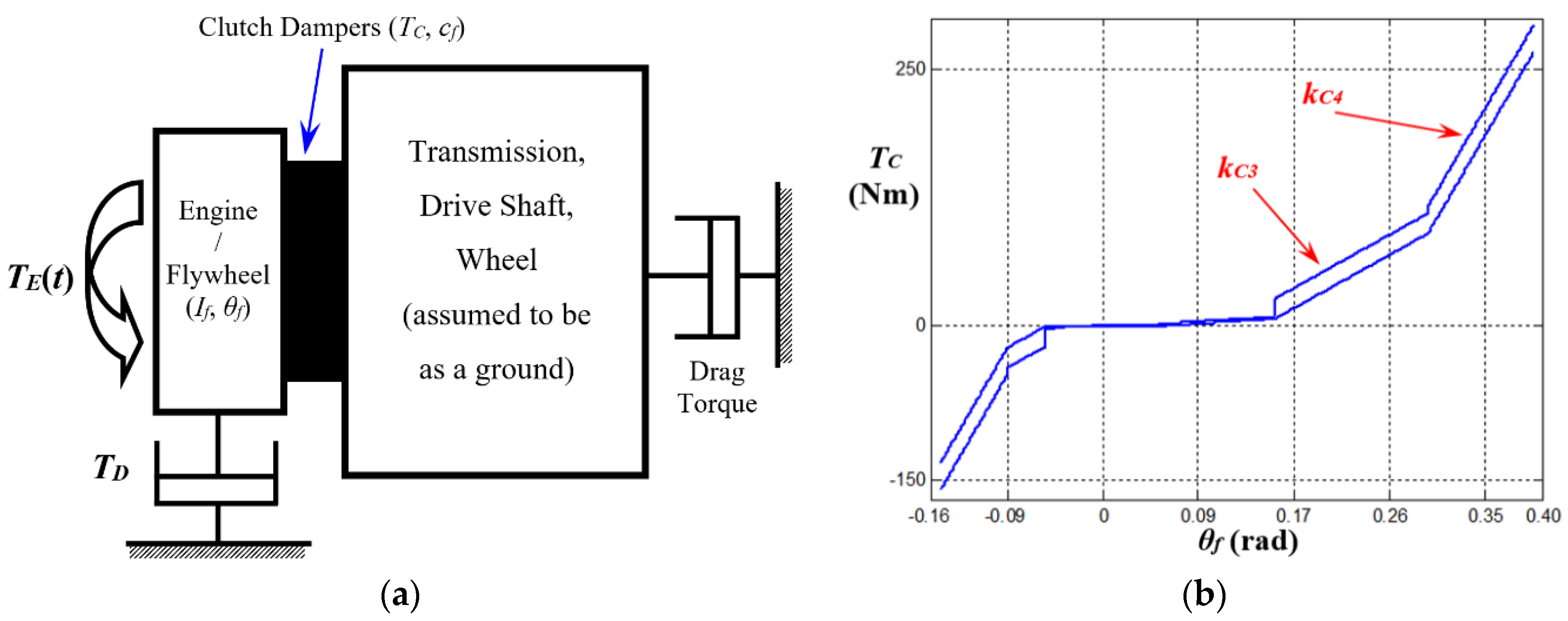
2. Problem Formulation with Multi-Staged Clutch Dampers
3. HBM with Modified Input Conditions
3.1. Basic Formulation of the HBM
3.2. Initial Results of the Basic HBM and Modification of the Input Conditions
4. Comparison of the Sub-Harmonic Responses from HBM and NS
5. Dynamic Characteristics with Bifurcation Diagrams in Sub-Harmonic Regimes
6. Conclusions
Author Contributions
Funding
Institutional Review Board Statement
Informed Consent Statement
Data Availability Statement
Conflicts of Interest
References
- Yoon, J.Y.; Singh, R. Effect of multi-staged clutch damper characteristics on transmission gear rattle under two engine conditions. Proc. IMechE Part D J. Automob. Eng. 2013, 227, 1273–1294. [Google Scholar] [CrossRef]
- Yoon, J.Y.; Yoon, H.S. Nonlinear frequency response analysis of a multistage clutch damper with multiple nonlinearities. ASME J. Comput. Nonlinear Dyn. 2014, 9, 031007. [Google Scholar] [CrossRef]
- Peng, Z.K.; Lang, Z.Q.; Bilings, S.A.; Tomlinson, G.R. Comparison between harmonic balance and nonlinear output frequency response function in nonlinear system analysis. J. Sound Vib. 2008, 311, 56–73. [Google Scholar] [CrossRef] [Green Version]
- Chen, Y.M.; Liu, J.K.; Meng, G. Incremental harmonic balance method for nonlinear flutter of an airfoil with uncertain-but-bounded parameters. Appl. Math. Model. 2012, 36, 657–667. [Google Scholar] [CrossRef]
- Al-shyyab, A.; Kahraman, A. Non-linear dynamic analysis of a multi-mesh gear train using multi-term harmonic balance method: Sub-harmonic motions. J. Sound Vib. 2005, 279, 417–451. [Google Scholar] [CrossRef]
- Masiani, R.; Capecchi, D.; Vestroni, F. Resonant and coupled response of hysteretic two-degree-of-freedom systems using harmonic balance method. Int. J. Non-Linear Mech. 2002, 37, 1421–1434. [Google Scholar] [CrossRef]
- Raghothama, A.; Narayanan, S. Bifurcation and chaos in geared rotor bearing system by incremental harmonic balance method. J. Sound Vib. 1999, 226, 469–492. [Google Scholar] [CrossRef]
- Raghothama, A.; Narayanan, S. Bifurcation and chaos of an articulated loading platform with piecewise non-linear stiffness using the incremental harmonic balance method. Ocean Eng. 2000, 27, 1087–1107. [Google Scholar] [CrossRef]
- Yang, Y.S.; Liu, X. Nonlinear dynamics of a spur gear pair with time-varying stiffness and backlash based on incremental harmonic balance method. Int. J. Mech. Sci. 2006, 48, 1256–1263. [Google Scholar]
- Duan, C.; Rook, T.E.; Singh, R. Sub-harmonic resonance in a nearly pre-loaded mechanical oscillator. Nonlinear Dyn. 2007, 50, 639–650. [Google Scholar] [CrossRef]
- Wong, C.W.; Zhang, W.S.; Lau, S.L. Periodic forced vibration of unsymmetrical piecewise-linear systems by incremental harmonic balance method. J. Sound Vib. 2006, 48, 1256–1263. [Google Scholar] [CrossRef]
- Kim, T.C.; Rook, T.E.; Singh, R. Super—And sub-harmonic response calculation for a torsional system with clearance nonlinearity using the harmonic balance method. J. Sound Vib. 2005, 281, 965–993. [Google Scholar] [CrossRef]
- Miguel, L.P.; Teloli, R.O.; Silva, S. Some practical regards on the application of the harmonic balance method for hysteresis models. Mech. Syst. Signal Process. 2020, 143, 106842. [Google Scholar] [CrossRef]
- Detroux, T.; Renson, L.; Masset, L.; Kerschen, G. The harmonic balance method for bifurcation analysis of large-scale nonlinear mechanical systems. Comput. Methods Appl. Mech. Eng. 2015, 296, 18–38. [Google Scholar] [CrossRef] [Green Version]
- Xie, L.; Baguet, S.; Prabel, B.; Dufour, R. Bifurcation tracking by Harmonic Balance Method for performance tuning of nonlinear dynamical systems. Mech. Syst. Signal Process. 2017, 88, 445–461. [Google Scholar] [CrossRef] [Green Version]
- Von Groll, G.; Ewins, D.J. The harmonic balance method with arc-length continuation in rotor/stator contact problems. J. Sound Vib. 2001, 241, 223–233. [Google Scholar] [CrossRef] [Green Version]
- Deconinck, B.; Nathan Kutz, J. Computing spectra of linear operators using the Floquet-Fourier-Hill method. J. Comput. Phys. 2006, 219, 296–321. [Google Scholar] [CrossRef]
- Lei, H.; Huizheng, C.; Yushu, C.; Kuan, L.; Zhansheng, L. Bifurcation and stability analysis of a nonlinear rotor system subjected to constant excitation and rub-impact. Mech. Syst. Signal Process. 2019, 125, 65–78. [Google Scholar]
- Lei, H.; Yushu, C. Analysis of 1/2 sub-harmonic resonance in a maneuvering rotor system. Sci. China Technol. Sci. 2014, 57, 203–209. [Google Scholar]
- Yoon, J.Y.; Byeongil, K. Stability and bifurcation analysis of super- and sub-harmonic responses in a torsional system with piecewise-type nonlinearities. Sci. Rep. 2021, 11, 1–18. [Google Scholar] [CrossRef]
- Dormand, J.R.; Prince, P.J. A family of embedded Runge-Kutta formulae. J. Comput. Appl. Math. 1980, 6, 19–26. [Google Scholar] [CrossRef] [Green Version]
- Seydel, R. Practical Bifurcation and Stability Analysis. Springer: Berlin/Heidelberg, Germany, 1994. [Google Scholar]
 , HBM result with = 2 and Nmax = 12;
  , NS result with frequency up-sweeping; +, NS result with frequency down-sweeping.
, HBM result with = 2 and Nmax = 12; , NS result with frequency up-sweeping; +, NS result with frequency down-sweeping.
, NS result with frequency up-sweeping; +, NS result with frequency down-sweeping.
, HBM result with = 2 and Nmax = 12; , NS result with frequency up-sweeping; +, NS result with frequency down-sweeping.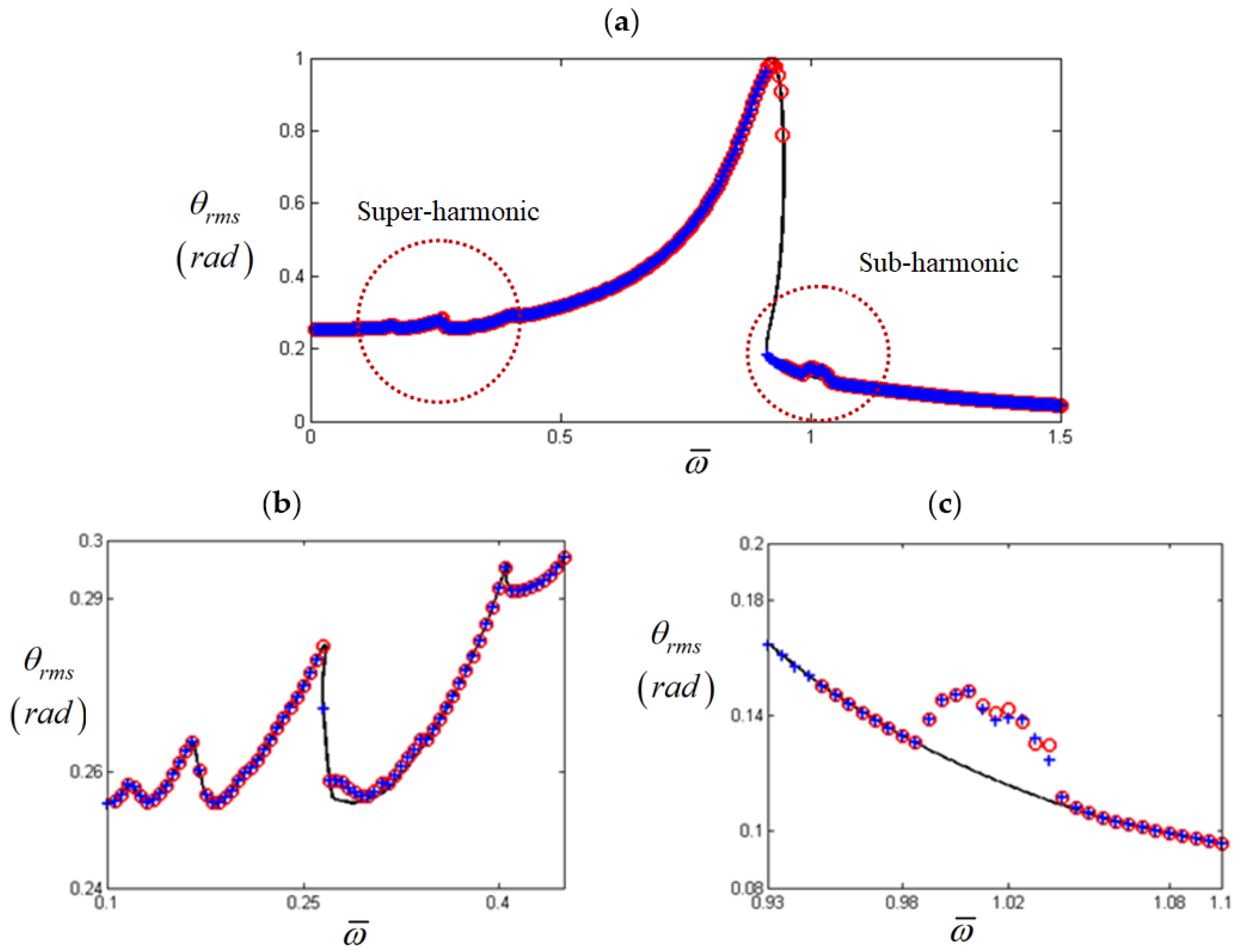
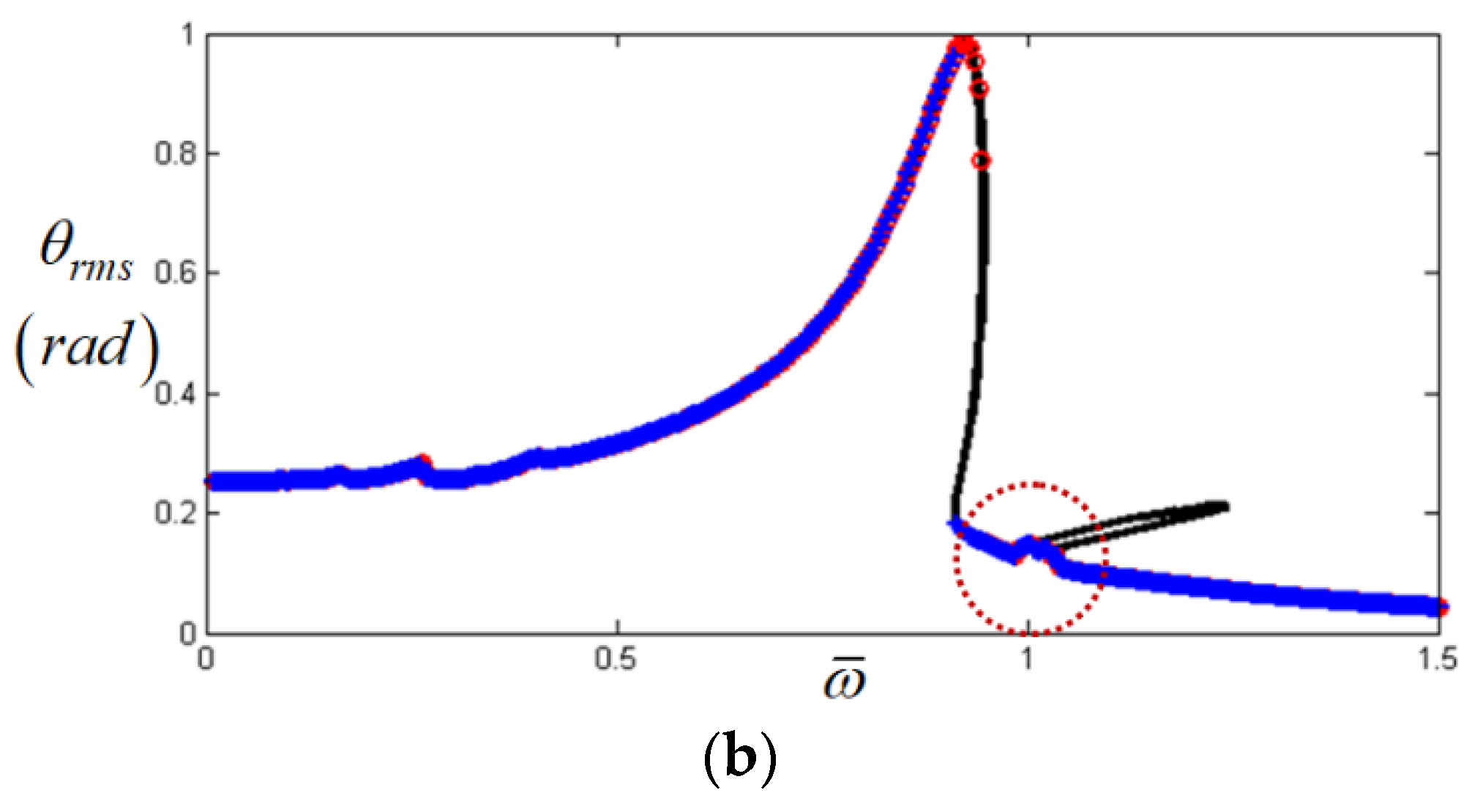
 , stable solution from HBM with Nmax = 12 and ρ = 2;
  , unstable solution from HBM with Nmax = 12 and ρ = 2; , NS result with frequency up-sweeping; +, NS result with frequency down-sweeping.
, stable solution from HBM with Nmax = 12 and ρ = 2; , unstable solution from HBM with Nmax = 12 and ρ = 2; , NS result with frequency up-sweeping; +, NS result with frequency down-sweeping.
, unstable solution from HBM with Nmax = 12 and ρ = 2; , NS result with frequency up-sweeping; +, NS result with frequency down-sweeping.
, stable solution from HBM with Nmax = 12 and ρ = 2; , unstable solution from HBM with Nmax = 12 and ρ = 2; , NS result with frequency up-sweeping; +, NS result with frequency down-sweeping.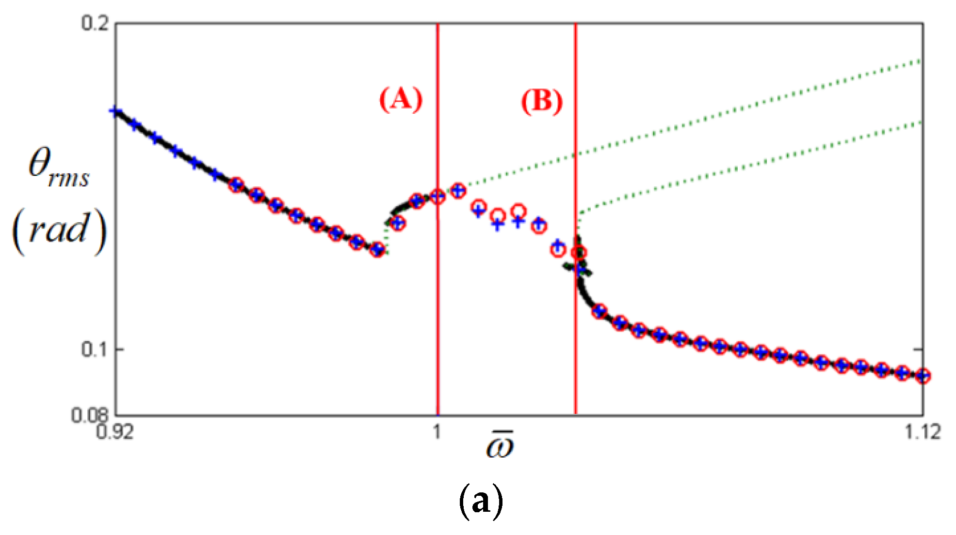
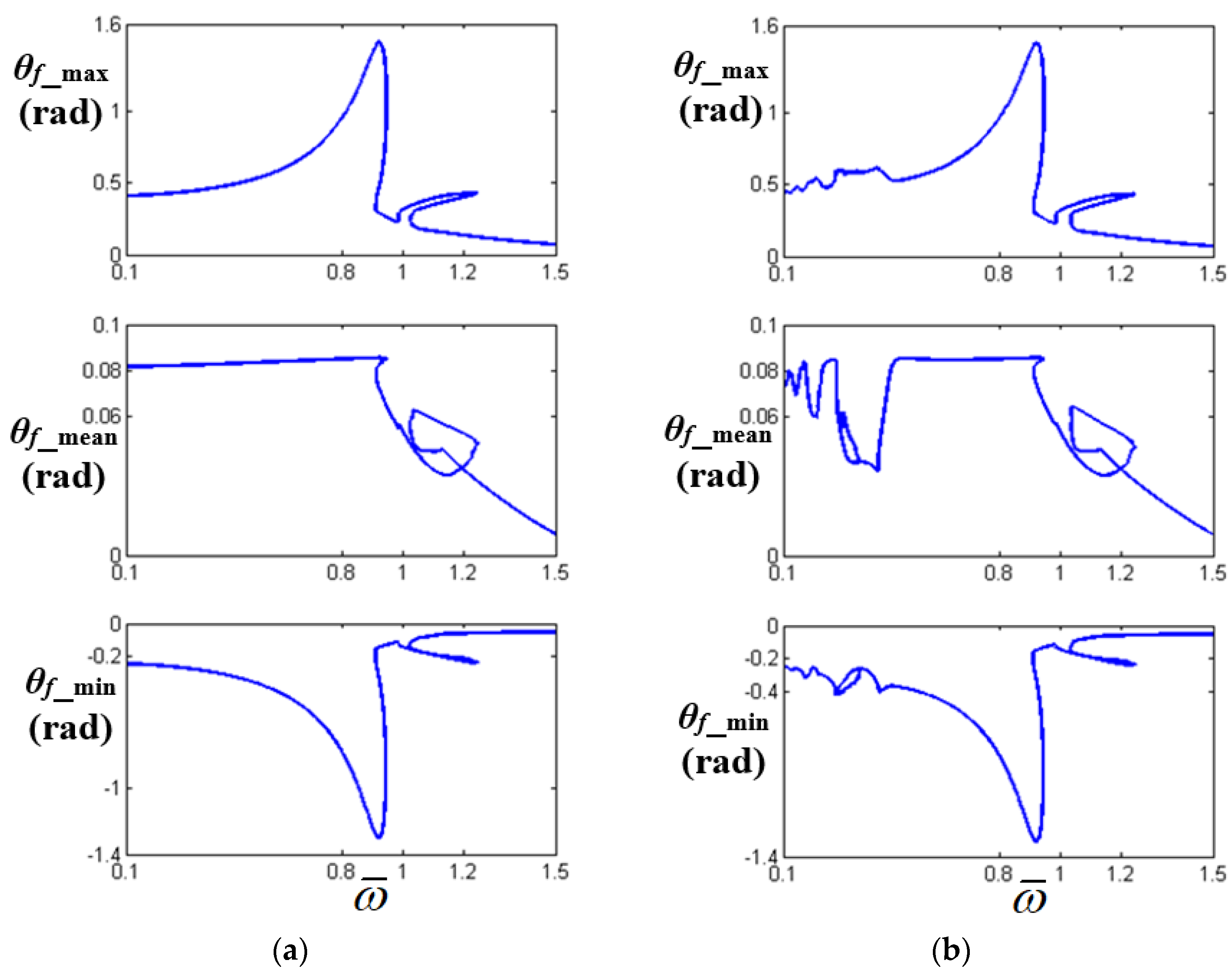
 , HBM;
  , NS.
, HBM; , NS.
, NS.
, HBM; , NS.
 , HBM;
  , NS.
, HBM; , NS.
, NS.
, HBM; , NS.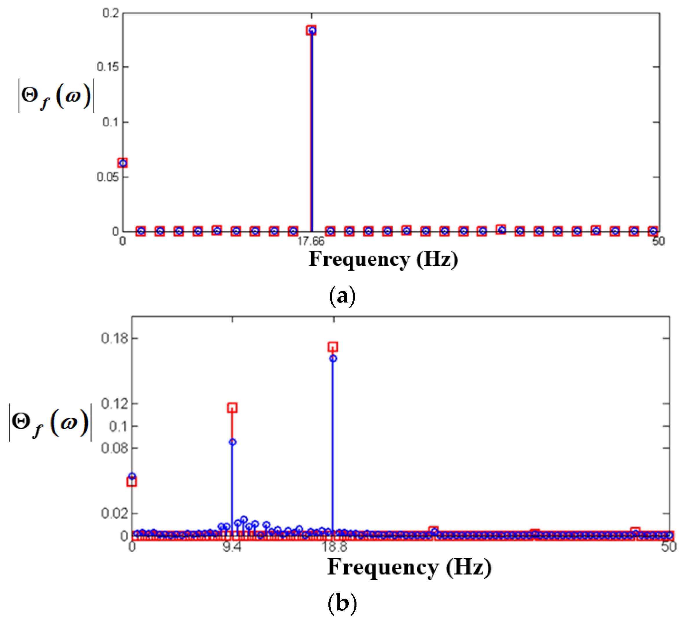
 , HBM; , NS.
, HBM; , NS.
, HBM; , NS.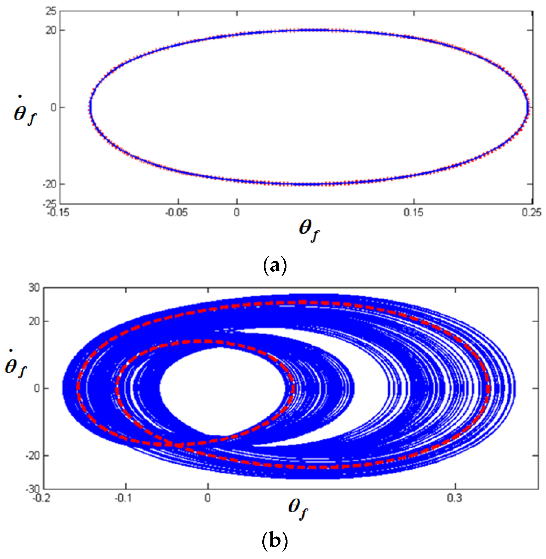 , stable solutions of HBM; +, unstable solutions of HBM;
  , numerical results of the bifurcation.
, stable solutions of HBM; +, unstable solutions of HBM; , numerical results of the bifurcation.
, numerical results of the bifurcation.
, stable solutions of HBM; +, unstable solutions of HBM; , numerical results of the bifurcation.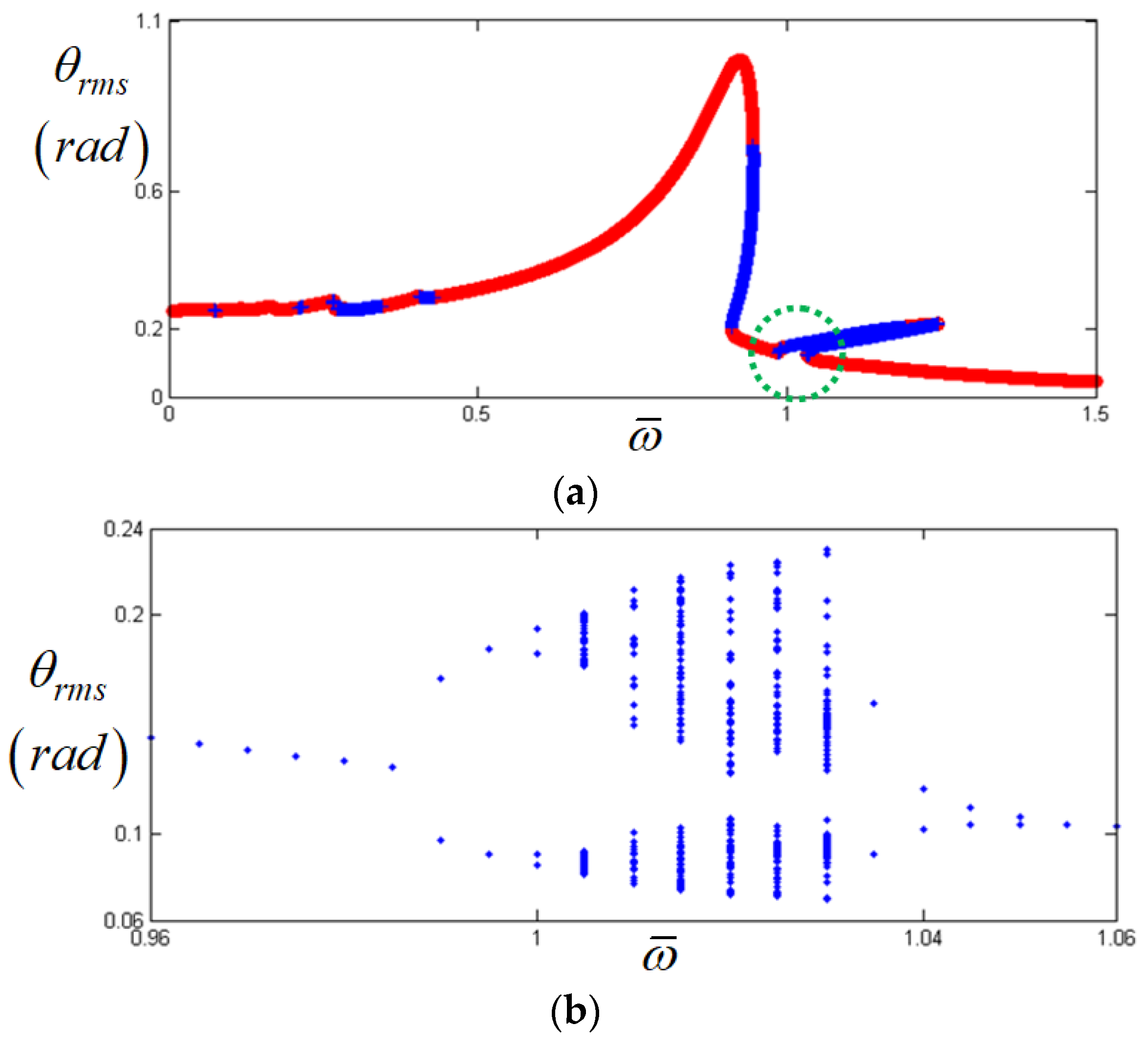 , stable solutions of HBM; +, unstable solutions of HBM; , numerical results of the bifurcation.
, stable solutions of HBM; +, unstable solutions of HBM; , numerical results of the bifurcation.
, stable solutions of HBM; +, unstable solutions of HBM; , numerical results of the bifurcation.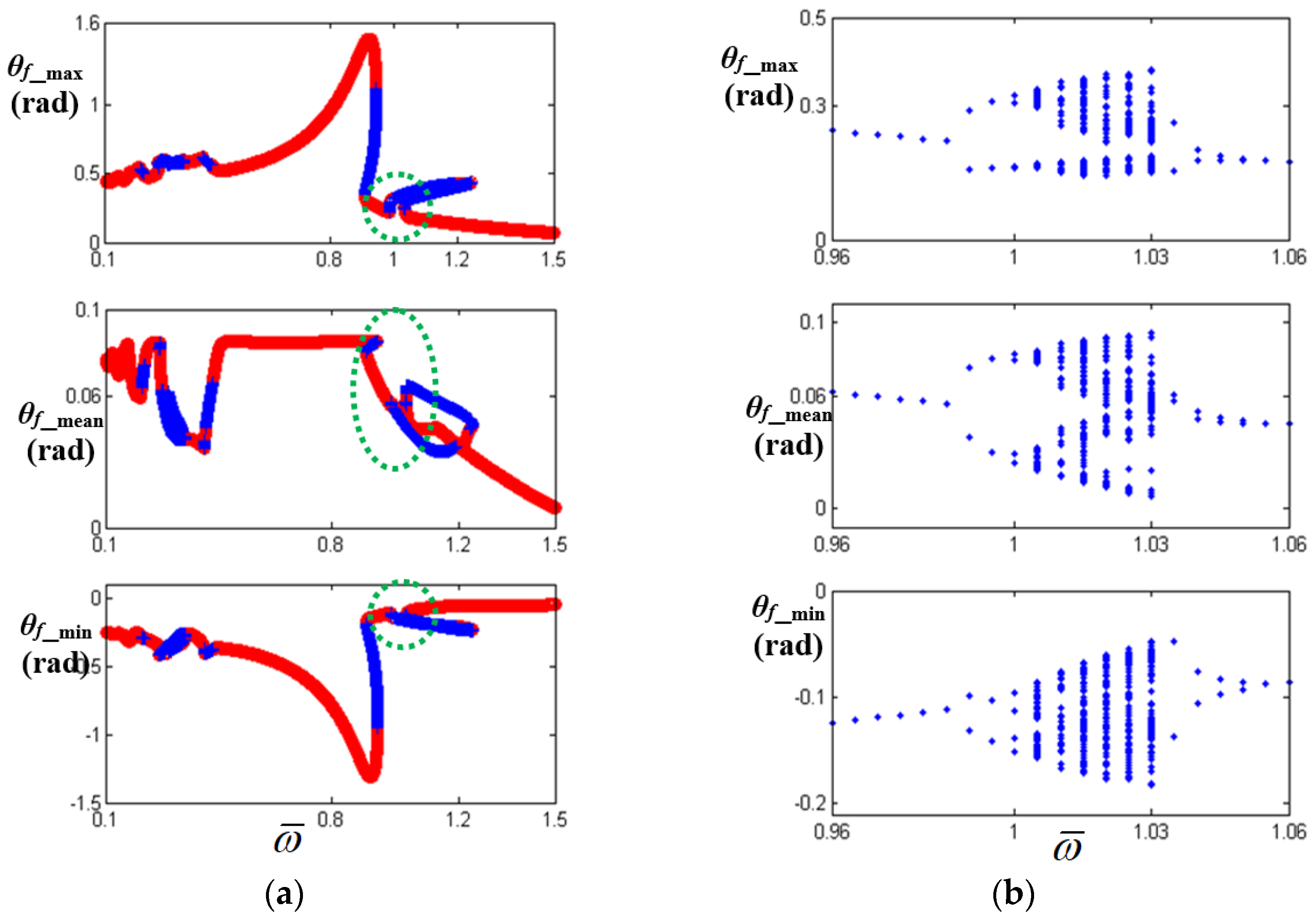 , stable solutions of HBM; +, unstable solutions of HBM; , numerical results of the bifurcations.
, stable solutions of HBM; +, unstable solutions of HBM; , numerical results of the bifurcations.
, stable solutions of HBM; +, unstable solutions of HBM; , numerical results of the bifurcations.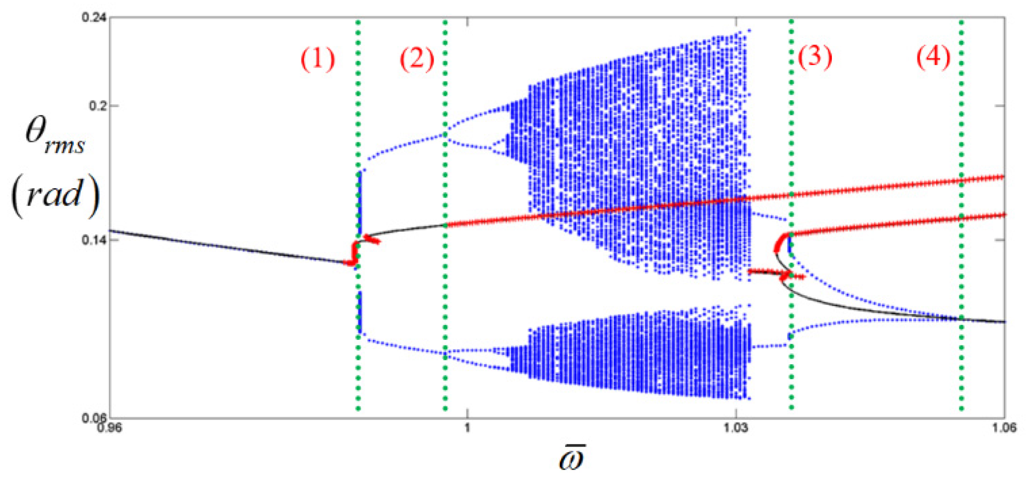 , stable solutions of HBM; +, unstable solutions of HBM; , numerical results of the bifurcations.
, stable solutions of HBM; +, unstable solutions of HBM; , numerical results of the bifurcations.
, stable solutions of HBM; +, unstable solutions of HBM; , numerical results of the bifurcations.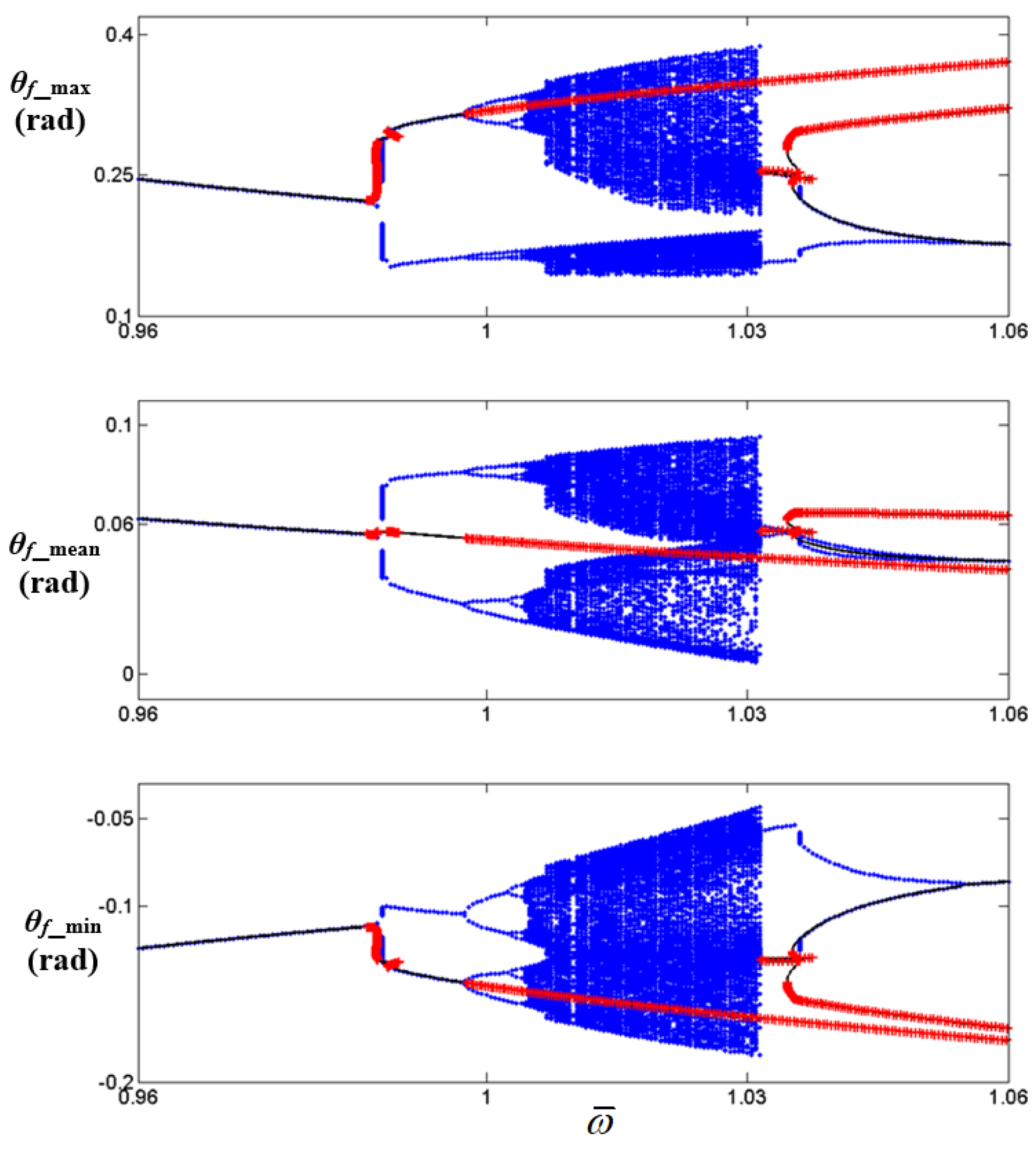

| Property | Stage | Value |
|---|---|---|
| Torsional stiffness, kCi (linearized in a piecewise manner) (Nm/rad) | 1 | 10.1 |
| 2 | 61.8 | |
| 3 | 595.8 | |
| 4 | 1838.0 | |
| Hysteresis, Hi (Nm) | 1 | 0.98 |
| 2 | 1.96 | |
| 3 | 19.6 | |
| 4 | 26.5 | |
| Transition angle at positive side (θf > 0), (rad) | 1 | 0.05 |
| 2 | 0.16 | |
| 3 | 0.30 | |
| 4 | 0.39 | |
| Transition angle at negative side (θf < 0), (rad) | 1 | −0.04 |
| 2 | −0.05 | |
| 3 | −0.09 | |
| 4 | −0.15 |
Publisher’s Note: MDPI stays neutral with regard to jurisdictional claims in published maps and institutional affiliations. |
© 2022 by the authors. Licensee MDPI, Basel, Switzerland. This article is an open access article distributed under the terms and conditions of the Creative Commons Attribution (CC BY) license (https://creativecommons.org/licenses/by/4.0/).
Share and Cite
Yoon, J.-Y.; Kim, B. Sub-Harmonic Response Analysis of Nonlinear Dynamic Behaviors Induced by Piecewise-Type Nonlinearities in a Torsional Vibratory System. Appl. Sci. 2022, 12, 1845. https://doi.org/10.3390/app12041845
Yoon J-Y, Kim B. Sub-Harmonic Response Analysis of Nonlinear Dynamic Behaviors Induced by Piecewise-Type Nonlinearities in a Torsional Vibratory System. Applied Sciences. 2022; 12(4):1845. https://doi.org/10.3390/app12041845
Chicago/Turabian StyleYoon, Jong-Yun, and Byeongil Kim. 2022. "Sub-Harmonic Response Analysis of Nonlinear Dynamic Behaviors Induced by Piecewise-Type Nonlinearities in a Torsional Vibratory System" Applied Sciences 12, no. 4: 1845. https://doi.org/10.3390/app12041845
APA StyleYoon, J.-Y., & Kim, B. (2022). Sub-Harmonic Response Analysis of Nonlinear Dynamic Behaviors Induced by Piecewise-Type Nonlinearities in a Torsional Vibratory System. Applied Sciences, 12(4), 1845. https://doi.org/10.3390/app12041845