Modern Methods and Techniques in Landscape Shaping with Various Functions on the Example of Southern Poland


Abstract
:1. Introduction
2. Materials and Methods
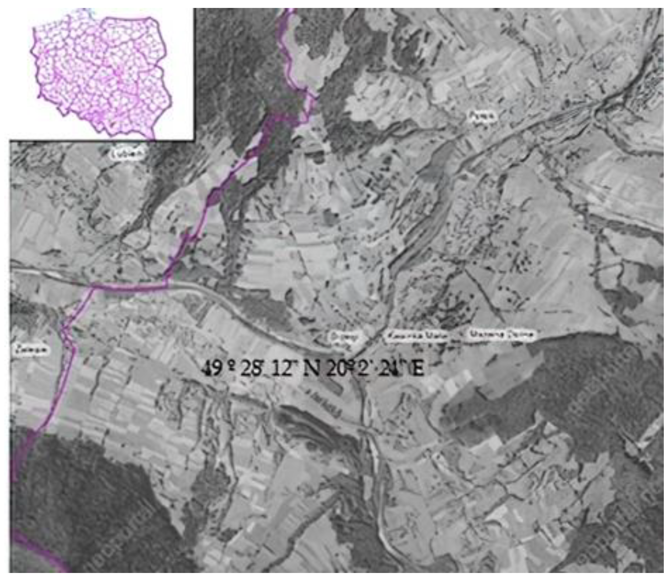
3. Area of Research
4. Selected Methods and Techniques in Landscape Assessment
4.1. WIT
- Average altitude—the average elevation of the location of the village.
- The soil quality index, calculated according to a 6-point scale by weighting the areas of agricultural land in each class with appropriate weights.
- The Steinhaus index of relief determines the degree of topographic differentiation of the terrain. The more intensive the terrain is, the higher the index is.
- The clustering index characterizes the degree to which the village area is filled with built-up land, i.e., it informs how much of the village area is built-up.
- The average distance between homesteads characterizes the internal spatial structure of a settlement.
- The settlement’s built-up area shape indicator expresses the ratio of the area’s maximum width to its length. For a square-shaped area, it equals 1 and decreases with lengthening.
- The number of homesteads per km2 characterizes the density of the rural settlement network.
- The average homestead size informs about the average size of an agricultural habitat in the area under consideration.
- The number of buildings; this indicator shows the total number of buildings in each settlement.
- Age of buildings built before 1944.
- Age of buildings constructed after 1944.
- Building material—non-flammable wall material indicates the number of buildings constructed with non-flammable materials (brick, concrete).
- Building material—combustible wall material indicates the number of buildings constructed with combustible materials (wood).
- Type of ownership determines the predominant character of ownership in a given area. Assumed: for private buildings −1, for non-private buildings 0.
- Area designated for building development (ha).
- Area allocated for communication (ha).
- Area for cultivation (ha).
- The indicator for the number of watercourses; it defines the ratio of the length of watercourses in a given village to its total area.
- Number of permanent residents.
- Percentage of people making their living from agriculture.
- Dominant terrain character: flat, undulating, hilly, mountainous.
- Special landscape values: landscape parks, protected landscape areas, protective forests, other.
- Predominant type of development: one-way compact, one-way loose, square multi-way, dispersed, urban.
- Number of individual farms with an area of 0.51–1.99 ha.
- Number of individual farms with an area of 2.00–9.99 ha.
- Number of individual farms with an area of 10 ha and more.
- Predominant types of plot layout: block-type, strip-type, block-strip-type.
- Presence of permanent terrain elements limiting the possibilities of plot layout changes: modification—none, escarpments, ravines, slopes, multi-year plantations, other.
- Land area under forests and woodlands.
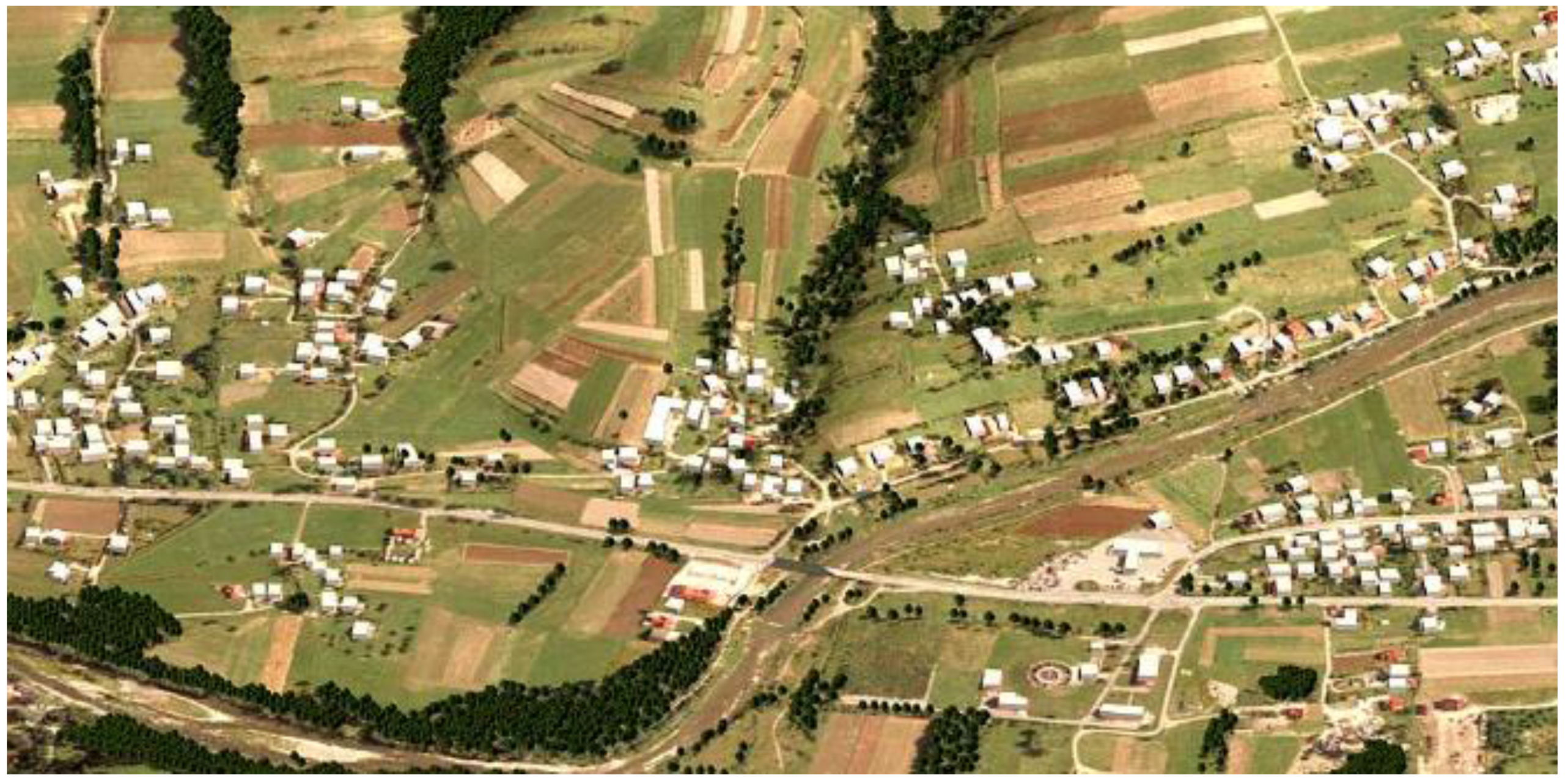
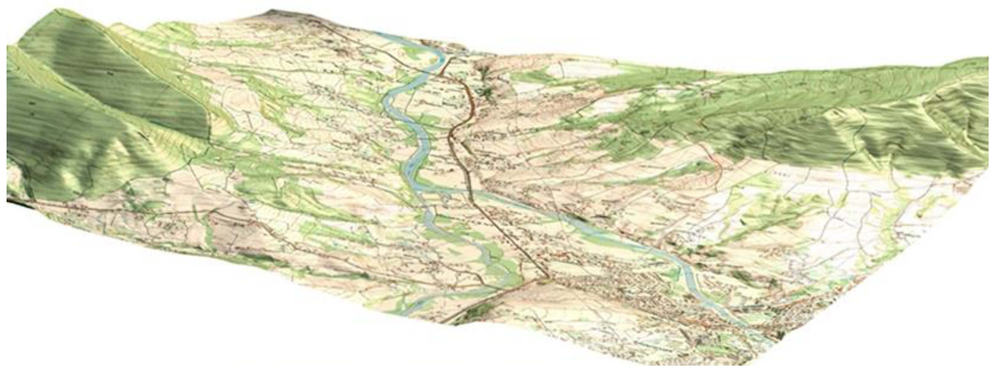
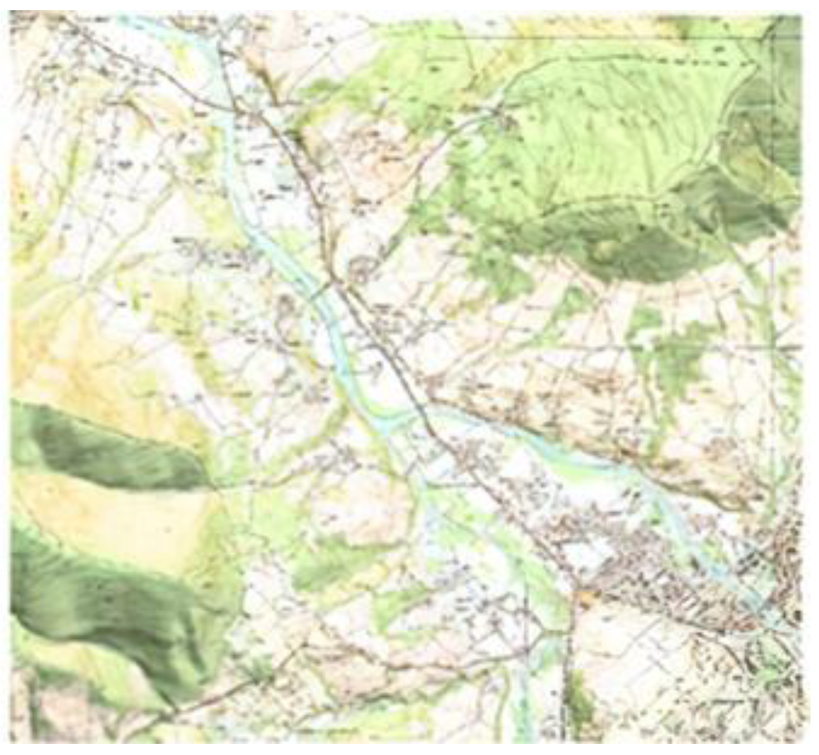
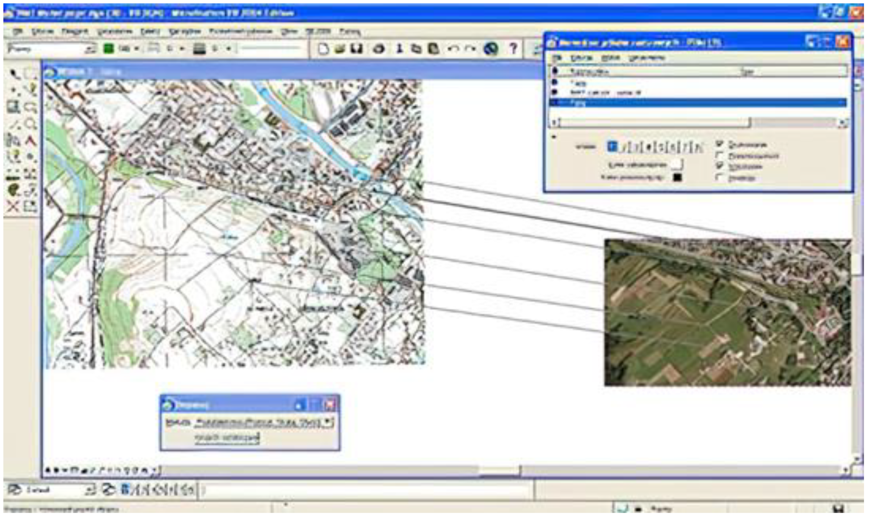
4.2. Orthophotomap
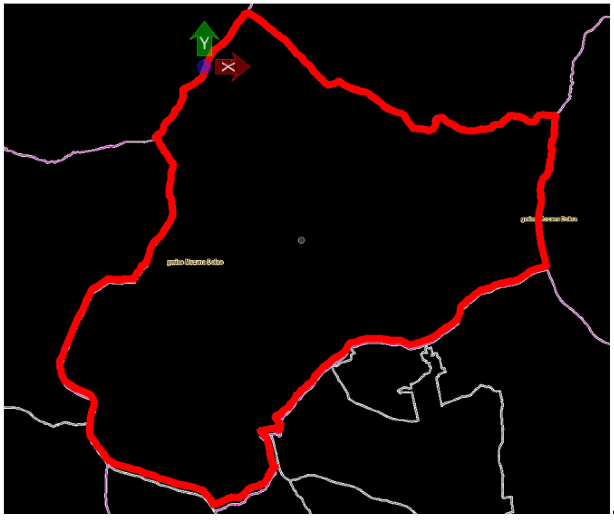
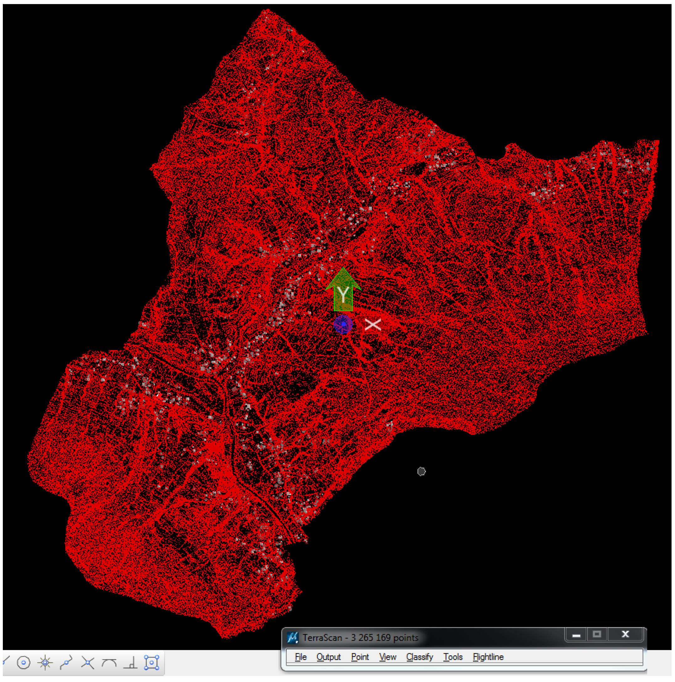
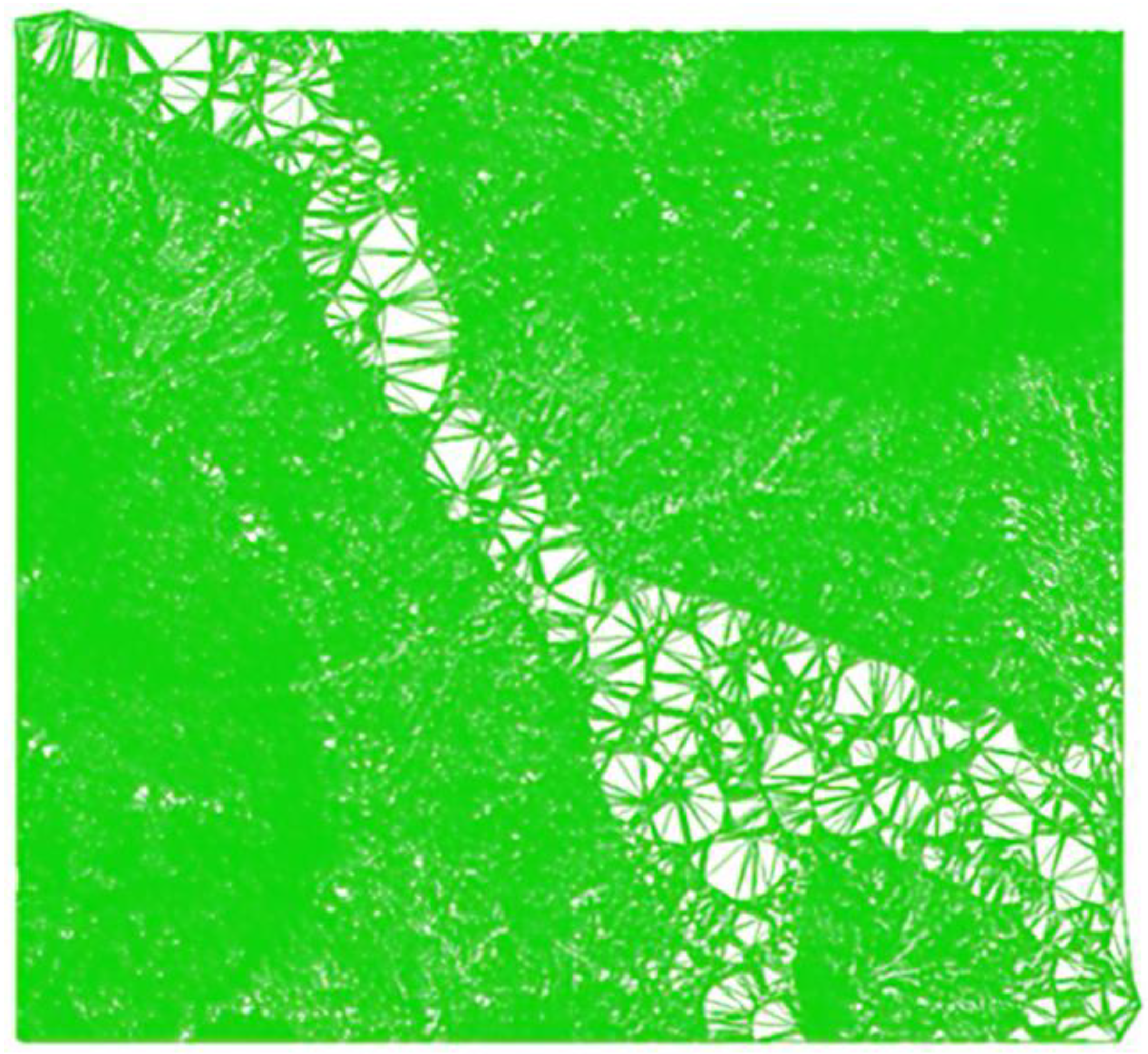
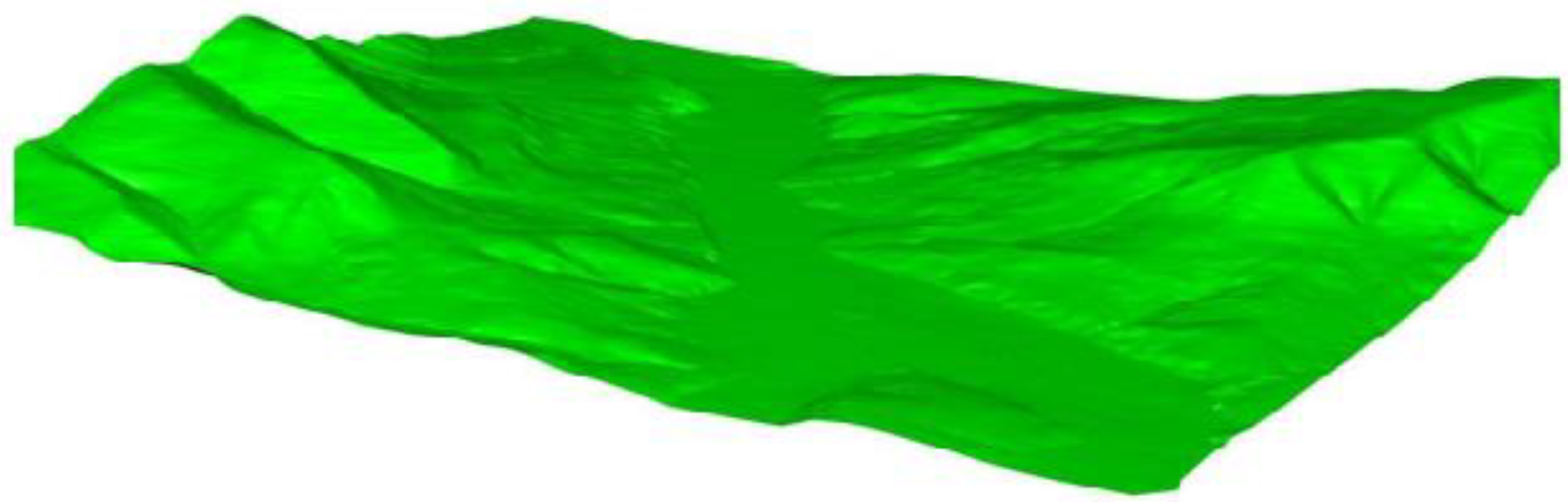
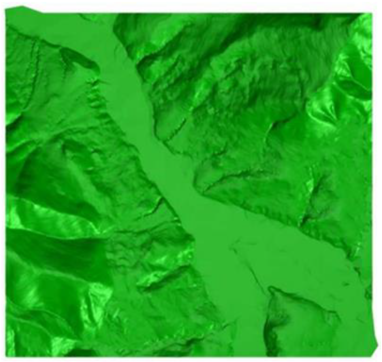
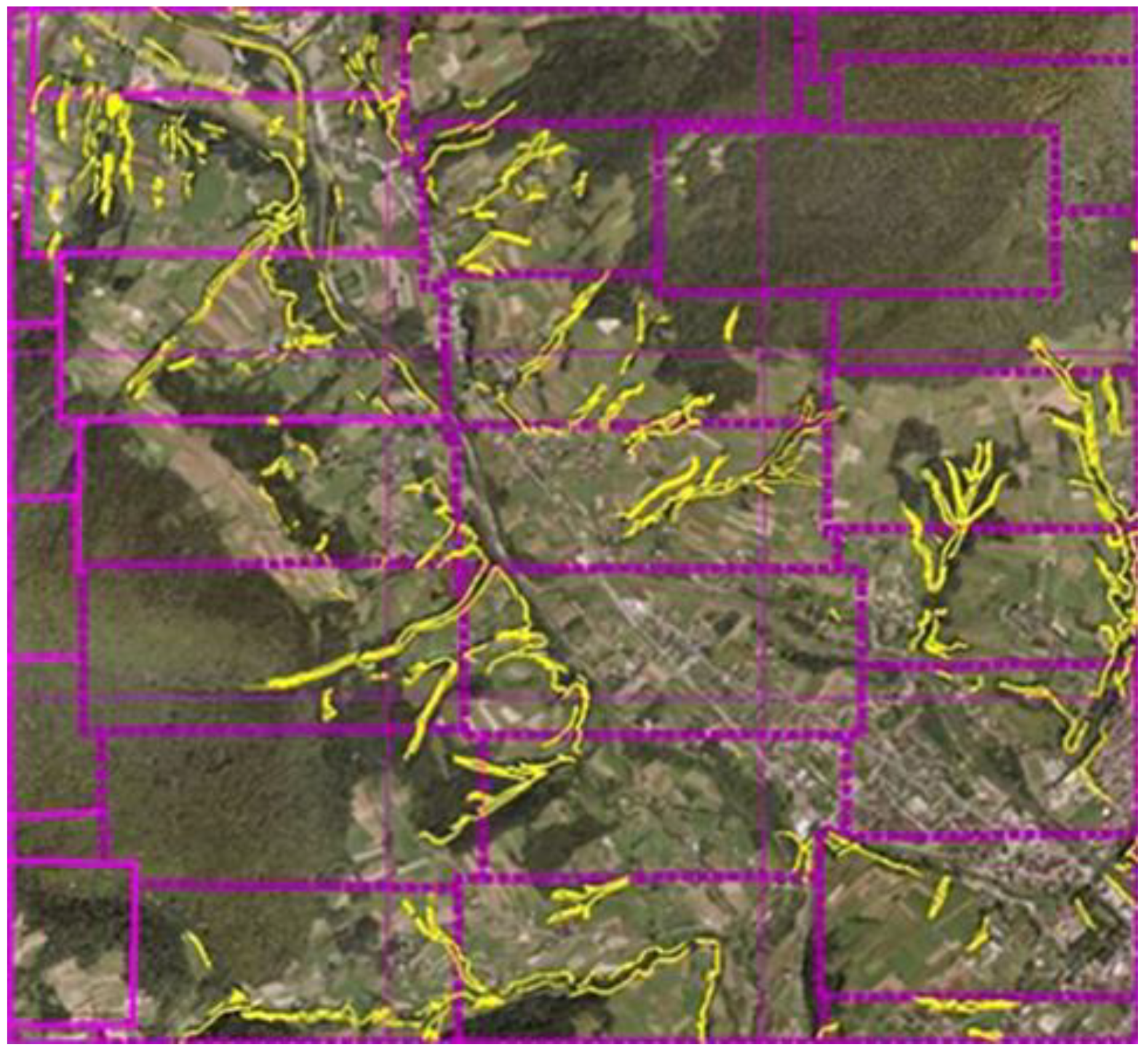
4.3. LIDAR in the Landscape Assessment
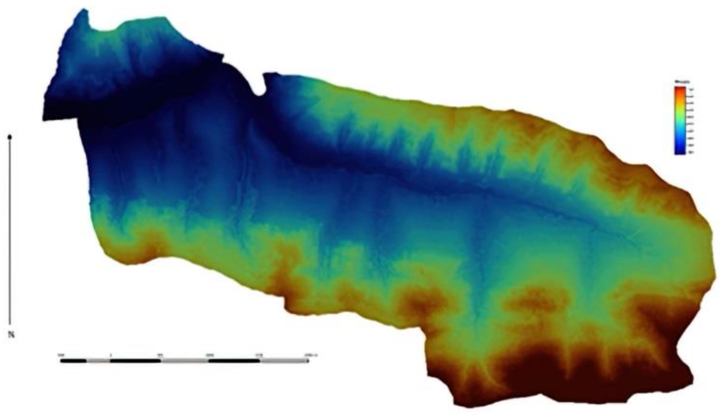
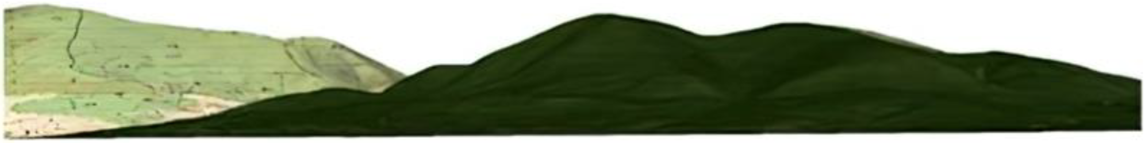
4.4. DTM and DSM
5. Results
5.1. Results Obtained Using the WIT
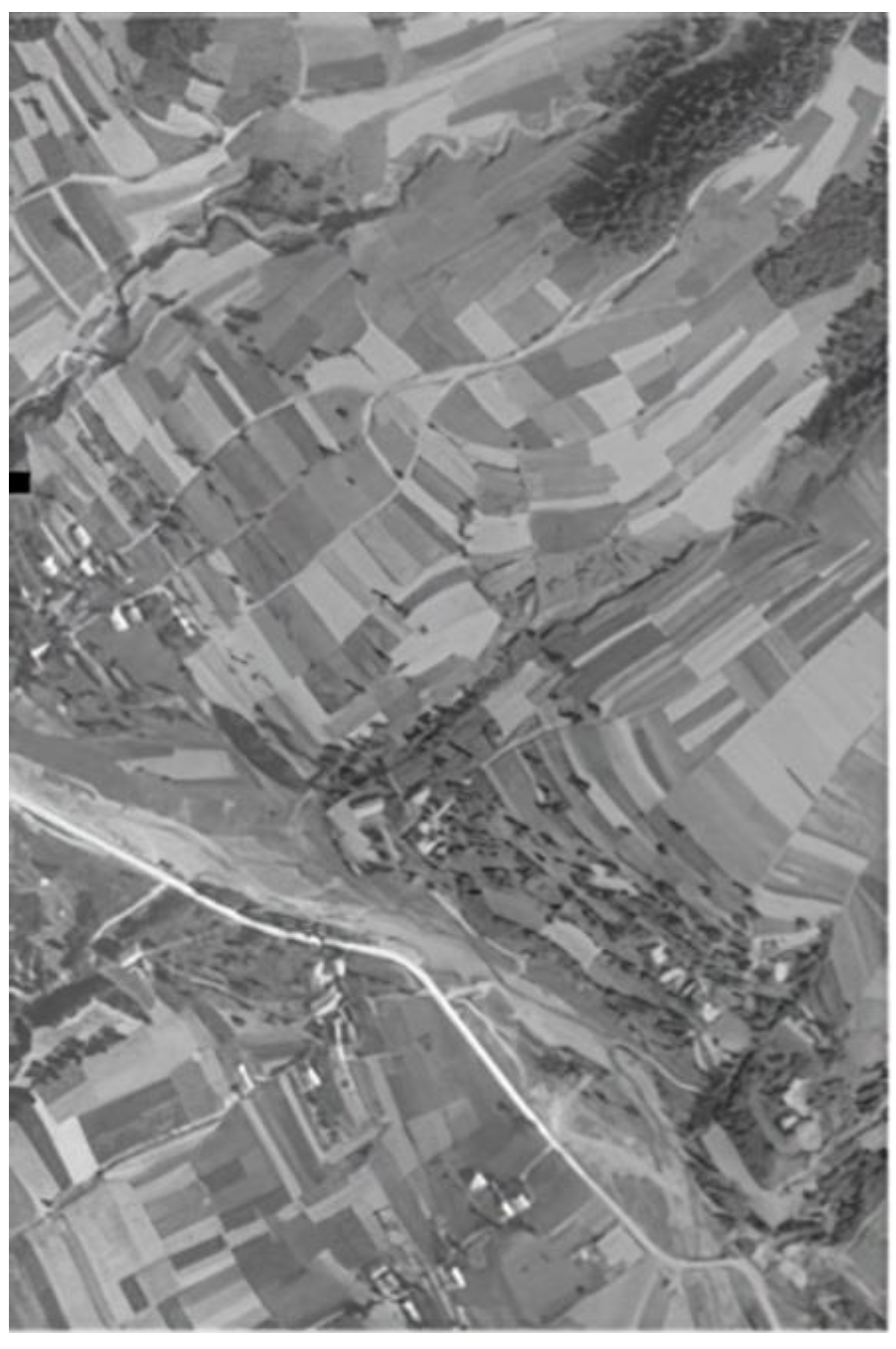
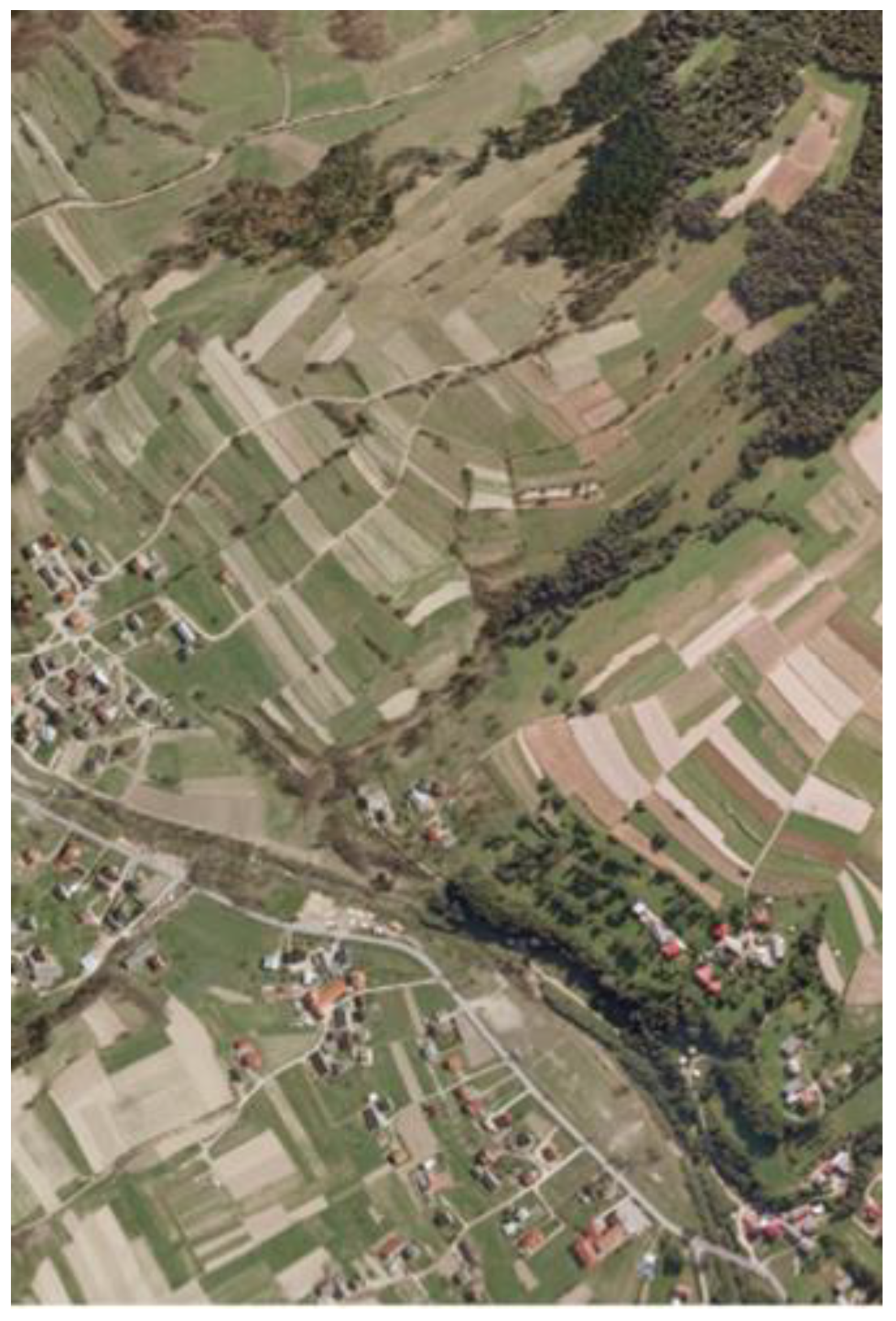
5.2. The Use of an Orthophotomap in Landscape Shaping
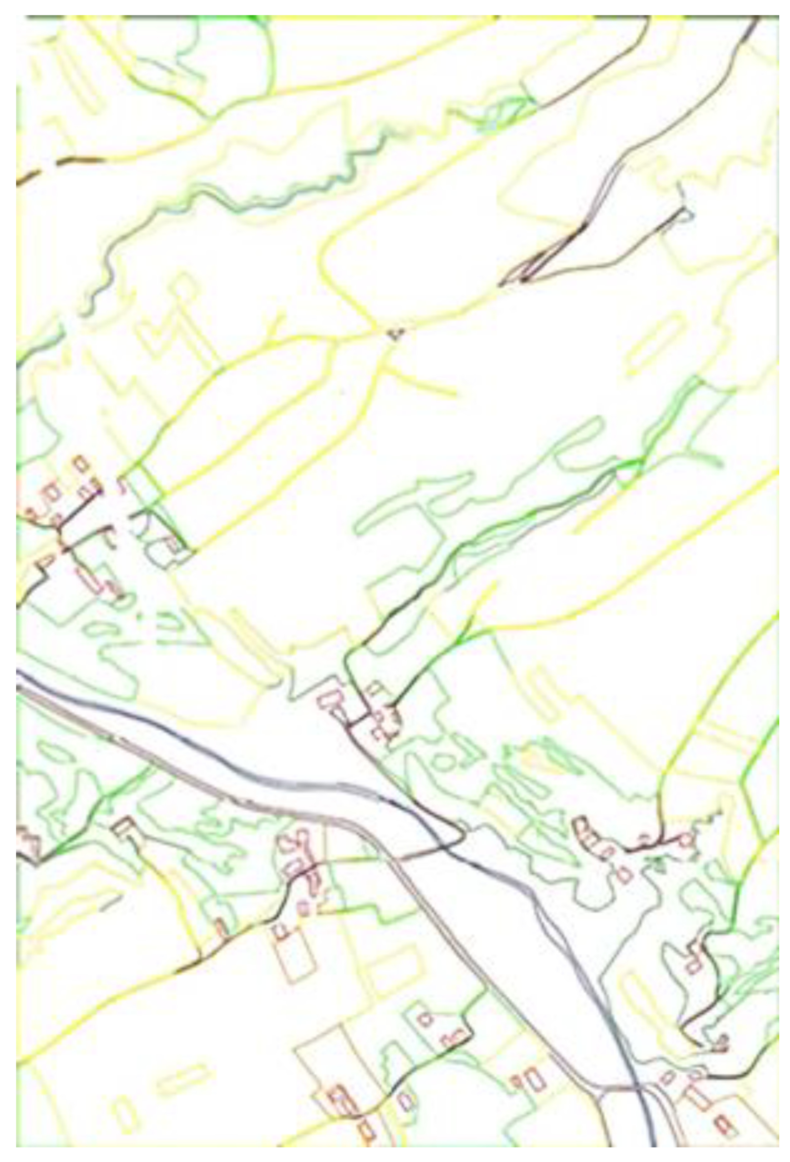
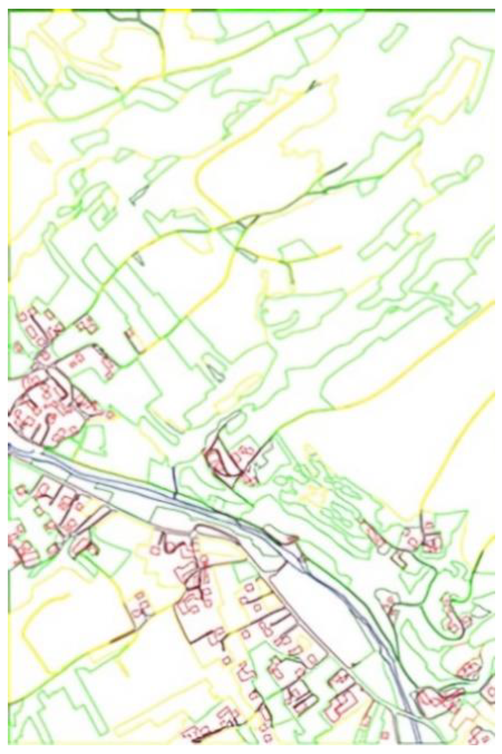
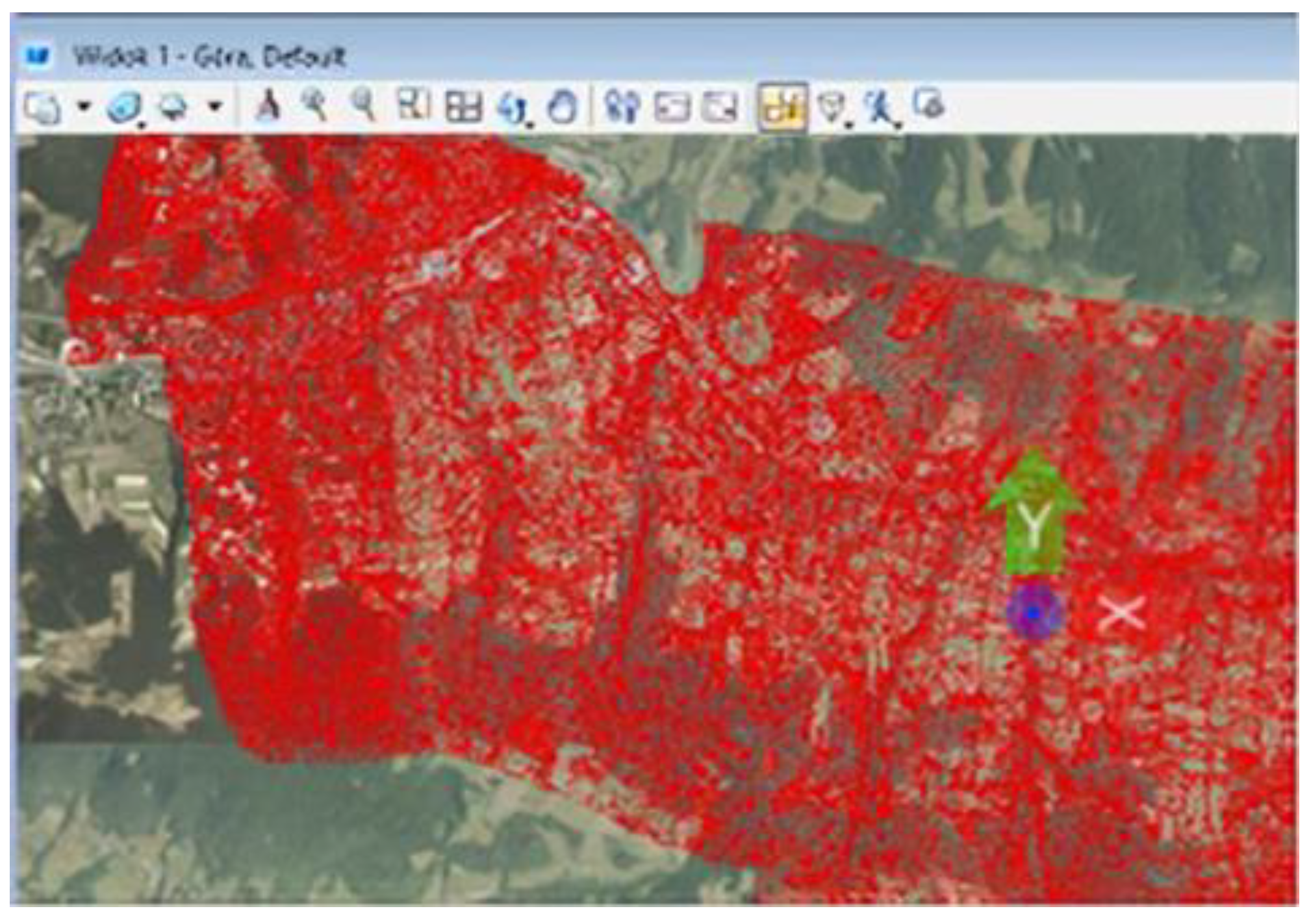
5.3. Results of the Study Using LIDAR
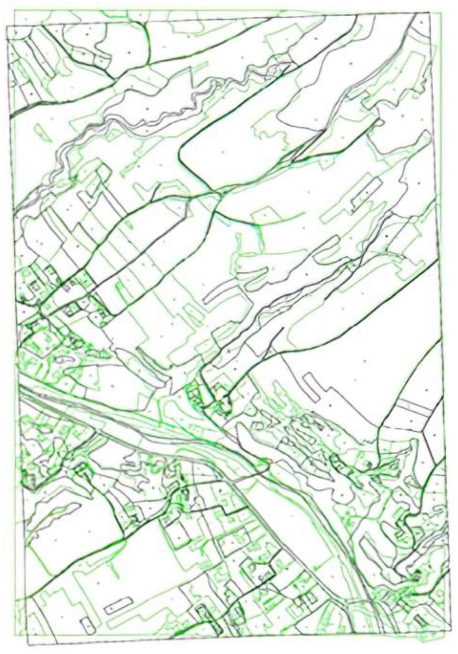
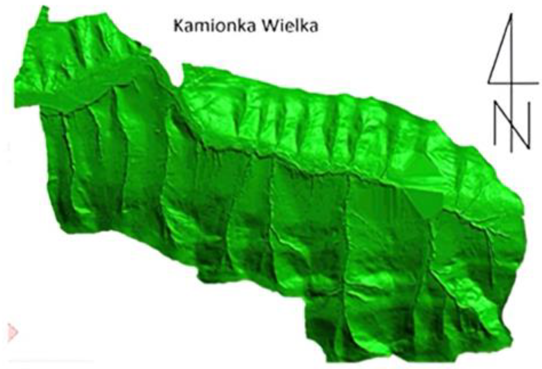
5.4. Results of the Study Using NMT, NMPT
5.5. Use of WIT and Photogrammetric Data in the Literature
6. Summary and Conclusions
- High-resolution aerial orthophotomaps are increasingly used to identify land cover changes.
- In conclusion, two aspects of the research work can be presented. One is related to the analysis of changes in selected landscape elements. The second is related to the technology that we can use in monitoring land cover changes. As far as the monitoring of changes is concerned, in the case of simple landscape elements, the use of aerial photographs seems obvious. As a result of the conducted research, it has turned out so, i.e., archival aerial photographs were an invaluable source of data in this case. One can even consider this kind of information exemplary.
- Landscape assessment methods based on digital image analysis are based, among others, on research using numerical models that present the surface of the terrain and/or its coverage, most often in the form of a regular GRID. The creation of such models for large areas requires a significant amount of data. Due to the speed of data registration in recent years, the unrivaled measurement method for surface modeling is airborne laser scanning. Acquired data, in the form of a dense point cloud, allow us to generate models with very high accuracy, which guarantees reliable results.
Author Contributions
Funding
Institutional Review Board Statement
Informed Consent Statement
Data Availability Statement
Conflicts of Interest
References
- Antrop, M. Why landscapes of the past are important for the future. Landsc. Urban Plan. 2005, 70, 21–34. [Google Scholar] [CrossRef]
- Bański, J. Geographies of Polish Rural Areas; Polish Economic Publishing House: Warsaw, Poland, 2006; Volume 155, pp. 30–35. [Google Scholar]
- Pietrzak, M. Landscape Syntheses—Assumptions, Problems, Applications; Bogucki Scientific Publishing: Poznan, Poland, 1998; Volume 119, pp. 17–19. [Google Scholar]
- Wojciechowski, K.H. Problems of Perception and Aesthetic Evaluation of the Landscape; Publishing House UMCS: Lublin, Poland, 1986; 283p. [Google Scholar]
- Wojciechowski, K.H. Landscapes—Elements of Cultural Heritage and Their Evolution; Series B; Annales UMCS: Lublin, Poland, 1996; Volume LI 19, pp. 287–297. [Google Scholar]
- Mazur, F. Natural Environment—Threats, Protection and Shaping; Publishing House of the University of Szczecin: Szczecin, Poland, 1998; 222p. [Google Scholar]
- Bogdanowski, J. Reading the Landscape. In National Heritage Landscapes; Number 1; Agencja Reklamowo-Wydawnicza A. Grzegorczyk: Stare Babice, Poland, 2000; pp. 7–18. ISSN 1509-961X. [Google Scholar]
- Meeus, J.H.A. Pau—European Landscapes. Landsc. Urban Plann. 1995, 31, 57–79. [Google Scholar] [CrossRef]
- Meeus, J.; Wijermans, M.; Vroom, M. Agricultural landscapes in Europe and their transformation. Landsc. Urban Plann. 1990, 18, 289–352. [Google Scholar] [CrossRef]
- Vos, W.; Meekes, H. Trends in European cultural landscape development: Perspectives for a sustainable future. Landsc. Urban Plann. 1999, 46, 3–14. [Google Scholar] [CrossRef]
- Cymerman, R. Rural Landscape; Publishing House ART: Olsztyn, Poland, 1992; 184p. [Google Scholar]
- Litwin, U. Indicator method for the evaluation of landscape structures. Sci. J. AR Krakow Sci. Sess. 1998, 335, 141–147. [Google Scholar]
- Magiera-Braś, G. Directions of land use against the background of natural constraints and the needs for works to improve agricultural space in mountain villages of the Krakow voivodeship. Sci. Pap. AR Krakow Geod. 1992, 264, 49–58. [Google Scholar]
- Wrona, A.; Truszkowski, L.; Dąbrowska, L. Environmental Evaluation of the Wielowieś Commune Part of I. State of Natural Values. In Environmental Protection Architecture; Number 1–2; ICE Publishing: London, UK, 1997; Volume 23, pp. 149–170. [Google Scholar]
- Journal of Laws Dz., U. 2001 No. 62 item 627 Act of April 27, 2001. Environmental Protection Law. Available online: https://isap.sejm.gov.pl (accessed on 1 December 2021).
- Majchrowska, A. Experience of other countries in identifying landscape types. In Identification and Valuation of Landscapes—Implementation of the European Landscape Convention; Conference papers; General Directorate for Environmental Protection: Warsaw, Poland, 2013. [Google Scholar]
- Jaszczuk, S.; Maj, K. Dictionary Geography; Greg Publishing House: Warsaw, Poland, 2004. [Google Scholar]
- Majchrowska, A. Landscape systematization in selected European countries. In The Problems of Landscape Ecology; Polska Asocjacja Ekologii Krajobrazu: Warsaw, Poland, 2008; Volume 20. [Google Scholar]
- Myczkowski, Z. Criteria for evaluation of Polish landscapes—A systematic proposal. In Identification and Valuation of Landscapes—Implementation of the European Landscape Convention; Conference papers; General Directorate for Environmental Protection: Warsaw, Poland, 2013. [Google Scholar]
- Bródka, S.; Macias, A. Stages of environmental assessment and their importance in the planning process. In Valorization of Natural Environment in Spatial Planning; Kistowski, M., Korwel-Lejkowska, B., Eds.; University of Gdańsk Development Foundation: Gdańsk, Warsaw, Poland, 2007. [Google Scholar]
- Kuraś, B. GIS technology as a complex tool in natural environment assessment studies on the example of Bielsko-Biała. Arch. Photogramm Cartog. Remote Sens. 2003, 13a, 119–127. [Google Scholar]
- Litwin, U. Determination of site importance indicators of the (WIT) Kotliny Mszańskiej. In Bulletin of the Agricultural Advisory Service AR Kraków; Number 314; Academy of Agriculture Krakow: Poland, 1997. [Google Scholar]
- Litwin, U.; Pijanowski, J.M. Active protection and shaping of cultural landscapes vs. valorization of their resources. In Scientific Quarterly No. 1 of the Higher School of Entrepreneurship in Nowy Sącz, Poland; Series: Geodesy and Cartography; Poland, 2008; pp. 37–43. [Google Scholar]
- Litwin, U. Synergic arrangement of landscape structures on the example of the Mszańska Basin. In Scientific Papers of the AR Krakow, Dissertations and Habilitations 225; Academy of Agriculture Krakow: Poland, 1997; p. 9. [Google Scholar]
- Jacobsen, K.; Passini, R. Accuracy of Digital Orthophotos from High Resolution Space Imagery. In Proceedings of the Workshop High Resolution Mapping from Space, Hanover, Germany, 23–25 December 2003. [Google Scholar]
- Forkuo, E.K. Digital terrain modeling in a GIS environment. In Remote Sensing and Spatial Information Sciences; ISPRS Archives part B2; Beijing 2008, China, Volume XXXVII, pp.1023-1030. Available online: https://citeseerx.ist.psu.edu/viewdoc/summary?doi=10.1.1.184.1603 (accessed on 1 December 2021).
- Longley, P.A.; Goodchild, M.F.; Maguire, D.J.; Rhind, D.W. GIS. Teoria i Praktyka; Wydawnictwo Naukowe PWN: Warsaw, Poland, 2006. [Google Scholar]
- Manuel, D.F. Digital Elevation Model Technologies and Applications. In The DEM Users Manual; ASPRS: Bethesda, MD, USA, 2001. [Google Scholar]
- Chrisman, N.R. Exploring Geographical Information Systems; Wiley: Hoboken, NJ, USA, 2003. [Google Scholar]
- Ballas, D.; Kingston, R.; Stillwell, J. Using a spatial microsimulation decision support system of policy scenario analysis. In Recent Advances in Design and Decision Support Systems in Atchitecture and Urban Planning; Kluwer Academic Publishers: Dordrecht, The Netherlands, 2004. [Google Scholar]
- Andrienko, N.; Andrienko, G.; Gatalsky, P. Exploratory spatiotemporal visualization: An analytical review. J. Vis. Lang. Comput. 2003, 14, 503–541. [Google Scholar] [CrossRef]
- Kopanakis, I.; Theodoulidis, B. Visual data mining modeling techniques for the visualization of mining outcomes. J. Vis. Lang. Comput. 2003, 14, 543–589. [Google Scholar] [CrossRef]
- Zhang, X.; Pazner, M. The icon imagemap technique for multivariate geospatial data visualization. Approach and software system. Cartogr. Geogr. Inf. Sci. 2004, 31, 29–41. [Google Scholar] [CrossRef]
- Andersen, H.-E. The Use of Airborne Laser Scanner Data (LIDAR) for Forest Measurement Applications; WFCA: Washington, DC, USA, 2002. [Google Scholar]
- Shan, J.; Toth, C.K. Topographic Laser Ranging and Scanning: Principles and Processing; CRC Taylor and Francis: Abingdon, UK, 2009. [Google Scholar]
- Naesset, E. Practical large-scale forest stand inventory using a smallfootprint airborne scanning laser. Scand. J. For. Res. 2004, 19, 164–179. [Google Scholar] [CrossRef]
- Ackermann, F. Airborne laser scanning—Present status and future expectations. J. Photogramm. Remote Sens. 1999, 54, 64–67. [Google Scholar] [CrossRef]
- Dunning, S.; Rosser, N.; Massem, C. The integration of terrestrial laser scanning and numerical modeling in landslide investigations. Quaterly J. Eng. Geol. Hydrogeol. 2010, 43, 233–247. [Google Scholar] [CrossRef]
- Doneus, M. Openness as Visualization Technique for Interpretative Mapping of Airborne Lidar Derived Digital Terrain Models. Remote Sens. 2013, 5, 6427–6442. [Google Scholar] [CrossRef] [Green Version]
- Vatan, M.; Oguz, M.; Selbesoglu Bayram, B. The use of 3D laser scanning technology in preservation of historical structures. Conservation News No 26/2009, pp. 659-669. Available online: https://www.researchgate.net/publication/235411453_The_Use_of_3D_Laser_Scanning_Technology_in_Preservation_of_Historical_Structures (accessed on 1 December 2021).
- Hyyppä, J.; Pyssalo, U.; Hyyppä, H.; Samberg, A. Elevation accuracy of laser scanning—Derived digital terrain and target models in forest environment. In International Archives of Photogrammetry and Remote Sensing; ISPRS Archives: Graz, Austria, 2002; Volume XXXIV/3A, Available online: https://www.researchgate.net/publication/237776901_Elevation_accuracy_of_laser_scanning-derived_digital_terrain_and_target_models_in_forest_environment (accessed on 1 December 2021).
- Hyyppä, J.; Mielonen, T.; Hyyppä, H.; Maltamo, M.; Yu, X.; Honkavaara, E.; Kaartinen, H. Using individual tree crown approach for forest volume extraction with aerial images and laser point clouds. In Proceedings of the ISPRS WG III/3, III/4, V/3 Workshop “Laser scanning 2005”, Enschede, the Netherlands, 12–14 September 2005; pp. 144–149. Available online: https://www.researchgate.net/publication/229029322_Using_individual_tree_crown_approach_for_forest_volume_extraction_with_aerial_images_and_laser_point_clouds (accessed on 1 December 2021).
- Morsdorf, F.; Meier, E.; Koetz, B.; Nüesch, D.; Itten, K.; Allgöwer, B. The potential of high resolution airborne laser scanning for deriving geometric properties of single trees. In Proceedings of the EGS—AGU—EUG Joint Assembly, Nice, France, 6–11 April 2003; Available online: https://www.researchgate.net/publication/252268314_The_potential_of_high_resolution_airborne_laser_scanning_for_deriving_geometric_properties_of_single_trees (accessed on 1 December 2021).
- Pitkänen, J.; Maltamo, M.; Hyyppä, J. Adaptive methods for individual tree detection on airborne laser based canopy height model. In International Archives of Photogrammetry, Remote Sensing and Spatial Information Sciences; ISPRS Archives: Freiburg, Niemcy, 2004; Volume XXXVI 8/W2, Available online: https://www.isprs.org/PROCEEDINGS/XXXVI/8-W2/PITKAENEN.pdf (accessed on 1 December 2021).
- Weinacker, H.; Kock, B.; Heyder, U.; Weinacker, R. Development of filtering, segmentation and modelling modules for LiDAR and multispectral data as a fundament of an automatic forest inventory system. In International Archives of Photogrammetry, Remote Sensing and Spatial Information Sciences; ISPRS Archives: Freiburg, Niemcy, 2004; Volume XXXVI 8/W2, Available online: https://citeseerx.ist.psu.edu/viewdoc/download?doi=10.1.1.215.2751&rep=rep1&type=pdf (accessed on 1 December 2021).
- Song, J.H.; Han, S.H.; Kim, Y.I. Assessing the possibility of land-cover classification using lidar intensity data. In International Archives of Photogrammetry and Remote Sensing; Graz, Austria, 2002; Volume XXXIV/3B, pp. 259–262. Available online: https://citeseerx.ist.psu.edu/viewdoc/download?doi=10.1.1.222.4122&rep=rep1&type=pdf (accessed on 1 December 2021).
- Kurczyński, Z. Airborne laser scanning in Poland—Between science and practice. Arch. Photogramm. Cartogr. Remote Sens. 2019, 31, 105–133. [Google Scholar] [CrossRef]
- Weibel, R.; Heller, M. Digital terrain modelling. In Geographical Information Systems: Principles and Applications; Maguire, D.J., Goodchild, M.F., Rhind, D.W., Eds.; Longman: London, UK, 1991; pp. 269–297. [Google Scholar]
- Andrienko, N.; Andrienko, G. Exploratory Analysis of Spatial and Temporal Data—A Systematic Approach; Springer: Berlin/Heidelberg, Germany, 2006. [Google Scholar]
- Dykes, J.; MacEachren, A.M.; Kraak, M.-J. Exploring geovisualization. In International Cartographic Association; Elsevier: Amsterdam, The Netherlands, 2005. [Google Scholar]
- Guo, D.; Gahegan, M.; MacEachren, A.M.; Zhou, B. Multivariate analysis and geovisualization with an integrated geographic knowledge discovery approach. Cartogr. Geogr. Inf. Sci. 2005, 32, 113–132. [Google Scholar] [CrossRef] [PubMed]
- Litwin, U.; Zawora, P. Spatial structure valuation with normalized land revelance indicators. In Acta Scientiarum Polonorum. Administratio Locorum 8/2; Olsztyn, Poland, 2009; pp. 15–27. Available online: https://czasopisma.uwm.edu.pl/index.php/aspal (accessed on 1 December 2021).
- Zawora, P.; Litwin, U. Valuing building land using economic indicators of site significance. In Acta Scientiarum Polonorum. Administratio Locorum 8/4; Olsztyn, Poland, 2009; pp. 33–40. Available online: https://czasopisma.uwm.edu.pl/index.php/aspal (accessed on 1 December 2021).
- Nita, J. The use of land surface numerical models and aerial photographs in the assessment of morphological forms for landscape valorization. Arch. Photogramm. Cartogr. Remote Sens. 2002, 12, 275–281. [Google Scholar]
- Kwoczynska, B.; Maślanka, K. Application of DEM and Digital Orthophotomap in Recording Changes Occurring in the Landscape on the Example of Domaniow Reservoir. In Geodesy Notebook; No 21; University of Agriculture: Krakow, Poland, 2005; Volume 417, pp. 249–260. [Google Scholar]
- Kwoczynska, B. Application of orthophotomap and digital terrain model for presentation of changes in ways of agricultural land use. Infrastruct. Ecol. Rural. Areas 2011, 3, 109–114. [Google Scholar]


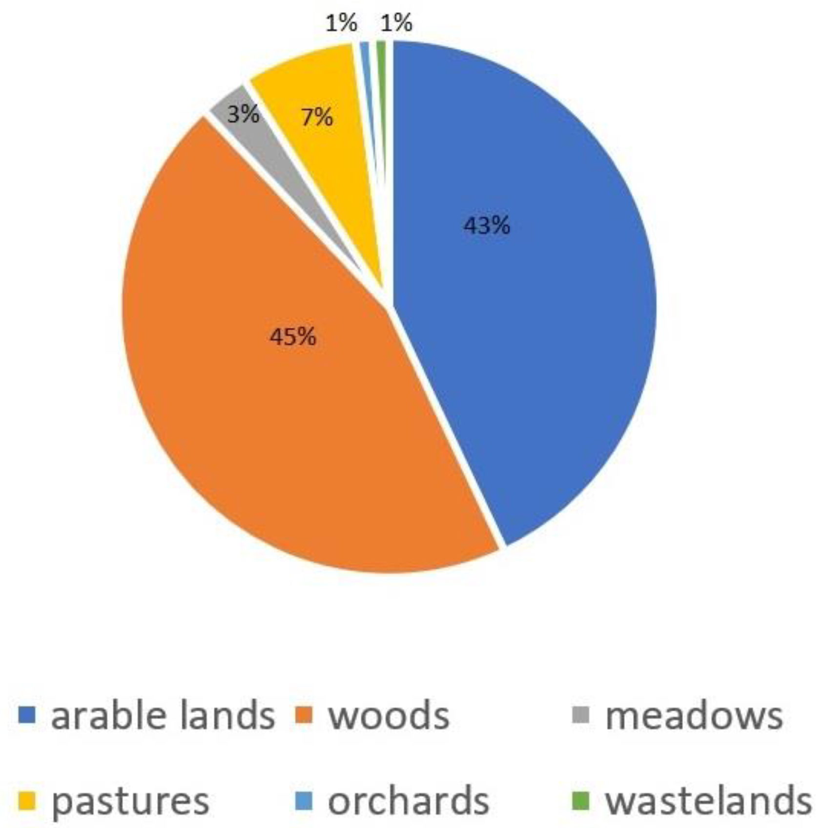
| Agricultural Land—1362 [ha], Including | |||||
|---|---|---|---|---|---|
| Arable Land [ha] | Orchards [ha] | Meadows [ha] | Pastures [ha] | Forests [ha] | Fallow Lands [ha] |
| 1077 | 32 | 68 | 185 | 1127 | 20 |
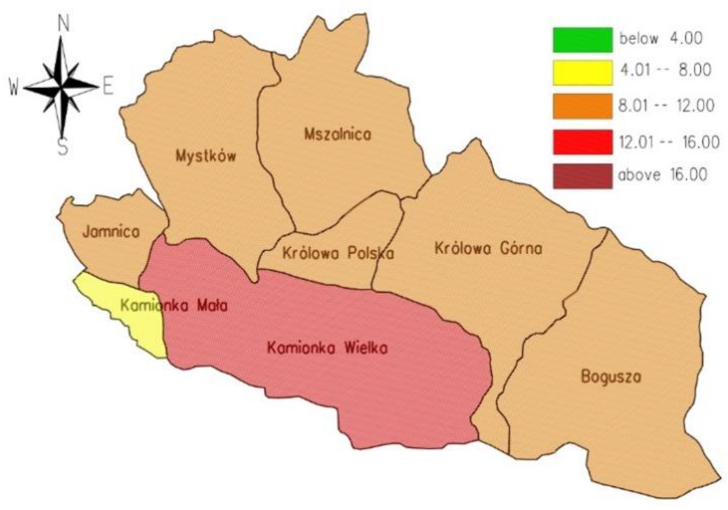
| No | Village | WIT 1 | WIT 2 | WIT 3 |
|---|---|---|---|---|
| 1 | Bogusza | 6.68 | 11.21 | 17.67 |
| 2 | Jamnica | 2.01 | 8.17 | 13.55 |
| 3 | Kamionka Mala | 1.05 | 4.99 | 12.97 |
| 4 | Kamionka Wielka | 0.55 | 14.69 | 24.80 |
| 5 | Królowa Górna | 9.33 | 11.50 | 20.42 |
| 6 | Królowa Polska | 5.17 | 8.37 | 15.07 |
| 7 | Mszalnica | 4.23 | 9.54 | 12.72 |
| 8 | Mystków | 0.74 | 10.90 | 15.69 |
| Type of Terrain | Area of the Site with an Orthophotomap from Year 1693 | Area of the Site with an Orthophotomap from Year 2010 |
|---|---|---|
| B | 0.8226 | 2.3574 |
| R | 58.4505 | 46.3167 |
| S | 1.9849 | 0.359 |
| W | 1.1482 | 0.7953 |
| x | 13.4925 | 10.1121 |
| Dr | 2.8649 | 3.5916 |
| Ls | 15.6849 | 26.8018 |
| Uz | 20.3064 | 24.421 |
| AMOUNT | 114.7549 | 114.7549 |
| Buildings | Arable Land | ||||
|---|---|---|---|---|---|
| Type of Terrain (1963) | Type of Terrain (2010) | Surface (ha) | Type of Terrain (1963) | Type of Terrain (2010) | Surface (ha) |
| B | B | 0.4747 | R | - | 0.7499 |
| B | Dr | 0.0300 | R | B | 0.278 |
| B | Ls | 0.0149 | R | Dr | 0.6233 |
| B | R | 0.0172 | R | Ls | 5.0166 |
| B | S | 0.0004 | R | R | 36.4486 |
| B | Uz | 0.0481 | R | Uz | 13.6086 |
| B | x | 0.2372 | R | x | 1.7255 |
| AMOUNT | 0.8225 | AMOUNT | 58.4505 | ||
| Grasslands | Water | ||||
| Type of Terrain (1963) | Type of Terrain (2010) | Surface (ha) | Type of Terrain (1963) | Type of Terrain (2010) | Surface (ha) |
| Uz | - | 0.3232 | W | - | 0.002 |
| Uz | B | 0.6257 | W | Dr | 0.0512 |
| Uz | Dr | 0.5390 | W | Ls | 0.8282 |
| Uz | Ls | 3.7568 | W | R | 0.0014 |
| Uz | R | 7.0737 | W | Uz | 0.0486 |
| Uz | S | 0.0038 | W | W | 0.0902 |
| Uz | Uz | 4.9715 | W | x | 0.1265 |
| Uz | x | 3.0127 | |||
| AMOUNT | 20.3064 | AMOUNT | 1.1481 | ||
| Forests | Orchards | ||||
| Type of Terrain (1963) | Type of Terrain (2010) | Surface [ha] | Type of Terrain (1963) | Type of Terrain (2010) | Surface [ha] |
| Ls | - | 0.1241 | S | - | 0.0356 |
| Ls | B | 0.2244 | S | B | 0.0671 |
| Ls | Dr | 0.2822 | S | Dr | 0.0214 |
| Ls | Ls | 11.0571 | S | Ls | 0.0782 |
| Ls | R | 0.7956 | S | R | 0.5827 |
| Ls | S | 0.0867 | S | S | 0.1039 |
| Ls | Uz | 1.8039 | S | Uz | 0.512 |
| Ls | x | 1.311 | S | x | 0.5842 |
| AMOUNT | 15.685 | AMOUNT | 1.9851 | ||
| Road | Other | ||||
| Type of Terrain (1963) | Type of Terrain (2010) | Surface [ha] | Type of Terrain (1963) | Type of Terrain (2010) | Surface [ha] |
| Dr | - | 0.0146 | x | - | 0.0035 |
| Dr | B | 0.0243 | x | B | 0.6269 |
| Dr | Dr | 1.1267 | x | Dr | 0.8441 |
| Dr | Ls | 0.646 | x | Ls | 3.7863 |
| Dr | R | 0.3496 | x | R | 0.1977 |
| Dr | S | 0.0164 | x | S | 0.1477 |
| Dr | Uz | 0.3281 | x | Uz | 2.3854 |
| Dr | W | 0.0067 | x | W | 0.6885 |
| Dr | x | 0.3524 | x | x | 4.8122 |
| AMOUNT | 2.8648 | AMOUNT | 13.4923 | ||
Publisher’s Note: MDPI stays neutral with regard to jurisdictional claims in published maps and institutional affiliations. |
© 2022 by the authors. Licensee MDPI, Basel, Switzerland. This article is an open access article distributed under the terms and conditions of the Creative Commons Attribution (CC BY) license (https://creativecommons.org/licenses/by/4.0/).
Share and Cite
Kwoczynska, B.; Litwin, U.; Piech, I. Modern Methods and Techniques in Landscape Shaping with Various Functions on the Example of Southern Poland. Appl. Sci. 2022, 12, 1948. https://doi.org/10.3390/app12041948
Kwoczynska B, Litwin U, Piech I. Modern Methods and Techniques in Landscape Shaping with Various Functions on the Example of Southern Poland. Applied Sciences. 2022; 12(4):1948. https://doi.org/10.3390/app12041948
Chicago/Turabian StyleKwoczynska, Boguslawa, Urszula Litwin, and Izabela Piech. 2022. "Modern Methods and Techniques in Landscape Shaping with Various Functions on the Example of Southern Poland" Applied Sciences 12, no. 4: 1948. https://doi.org/10.3390/app12041948
APA StyleKwoczynska, B., Litwin, U., & Piech, I. (2022). Modern Methods and Techniques in Landscape Shaping with Various Functions on the Example of Southern Poland. Applied Sciences, 12(4), 1948. https://doi.org/10.3390/app12041948