The greedy randomized adaptive search procedure algorithm (GRASP) is a metaheuristic proposed by Feo et al. [
26,
27]. The GRASP algorithm is a multi-start process that has two phases. The first phase corresponds to a heuristic construction, which provides a high-quality solution, and the second phase improves the solution through a local search. However, given the nature of the solution, a slight change in the placement of the rectangular objects for an already-completed solution would produce a huge problem for repairing highly-possible overlaps or would increase wastes. Therefore, we avoid the use of local search, limiting the algorithm to the heuristic construction phase.
Algorithm 1 shows the general procedure of our proposed optimization method; it generates the solutions with a defined number of iterations. The process starts with the
LoadInstance function that loads the instance. The
InitializeParameters function initializes the main parameters to use in GRASP construction. The
ReorderObjects function consists of ordering the objects from the smallest area to the largest area. The
SPPGRASP function constructs the GRASP solutions; we validate the solutions to obtain the best solution. This code is available at
https://github.com/csalas07/GraspSpp (accessed on 4 February 2022).
| Algorithm 1 GRASP General Procedure |
- 1:
, - 2:
LoadInstance() - 3:
InitializeParameters() - 4:
ReorderObjects() - 5:
for do - 6:
- 7:
if then - 8:
- 9:
end if - 10:
end for
|
| Output: best |
3.1. GRASP Construction
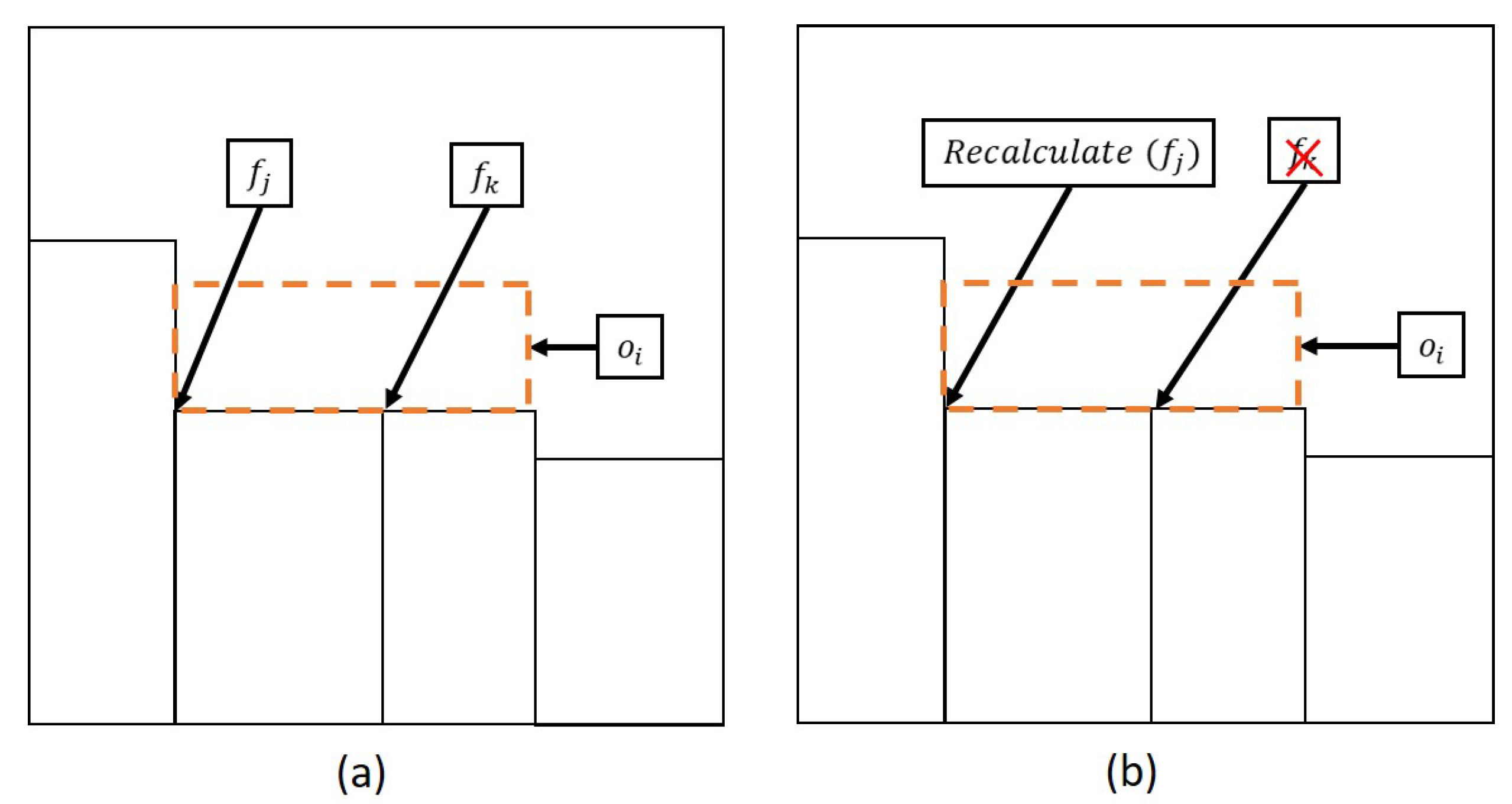
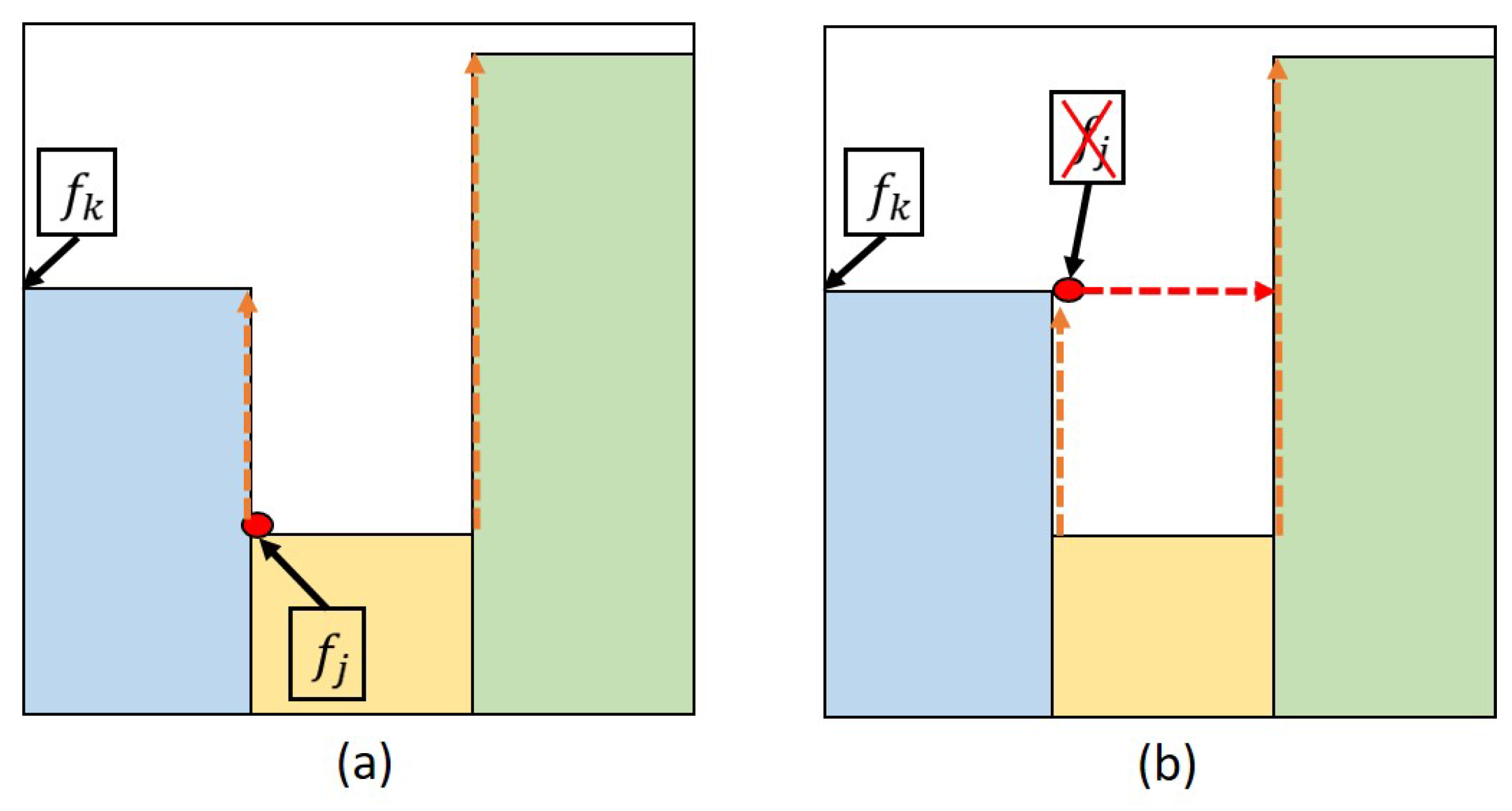
One of the main contributions of this paper is the use of flags, and at the beginning of the algorithm, we set a single flag at the lowest left corner of the strip to mark the first place for setting an object.
Algorithm 2 describes the initial construction that consists of three parts. The first is to select an available flag index with the
FindFlagIndex function (see line 4), which iterates a list of available flags and selects the index of the flag that has the lowest height, and if there were several flags with the same height, it chooses the one furthest to the left. The second part consist of the use of waste functions (see Equations (
5)–(
7)) to analyze the objects’ waste. Finally, the last part is constructing the candidate list (
CL) and the restricted candidate list (
RCL).
| Algorithm 2 GRASP Construction Part 1 |
Input:k- 1:
- 2:
while do - 3:
- 4:
- 5:
for do - 6:
if && then - 7:
- 8:
- 9:
- 10:
end if - 11:
end for - 12:
if then - 13:
- 14:
- 15:
- 16:
for do - 17:
- 18:
- 19:
- 20:
- 21:
end for - 22:
- 23:
for do - 24:
if then - 25:
- 26:
- 27:
end if - 28:
end for - 29:
|
The algorithm checks that the set value
is equal to zero, where
is a set that represents the availability of the objects (see Equation (
4)).
The
function calculates the waste area of an object
(see line 8). We use three waste functions (see Equations (
5)–(
7)) to analyze the objects’ waste. Each function validates different components among the rectangular objects and a specific flag.
where
is the set of objects and
is the waste of the object
i on the flag
j. Hence, in the algorithm, we calculate the waste for all the available objects
for the selected flag
.
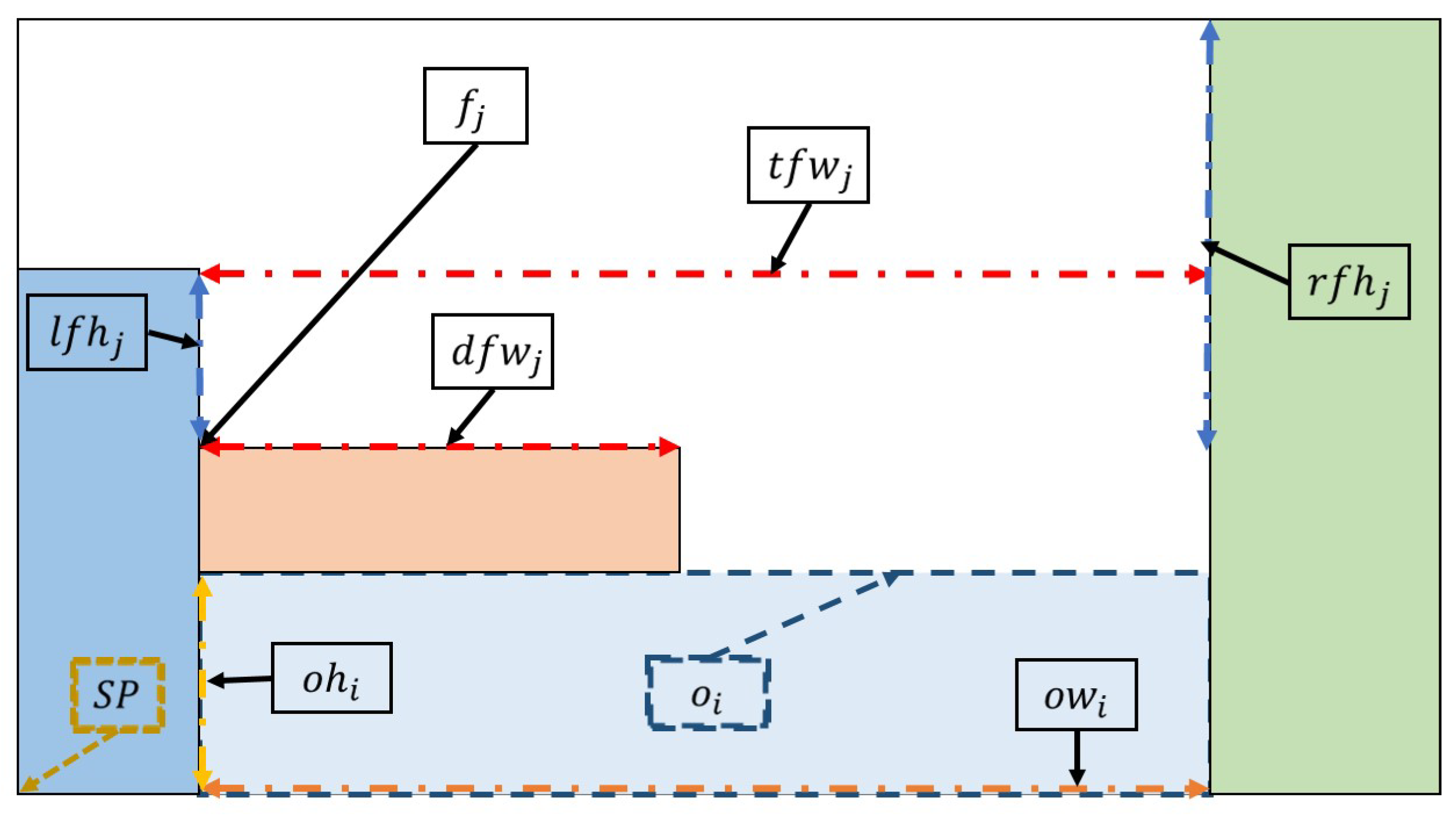
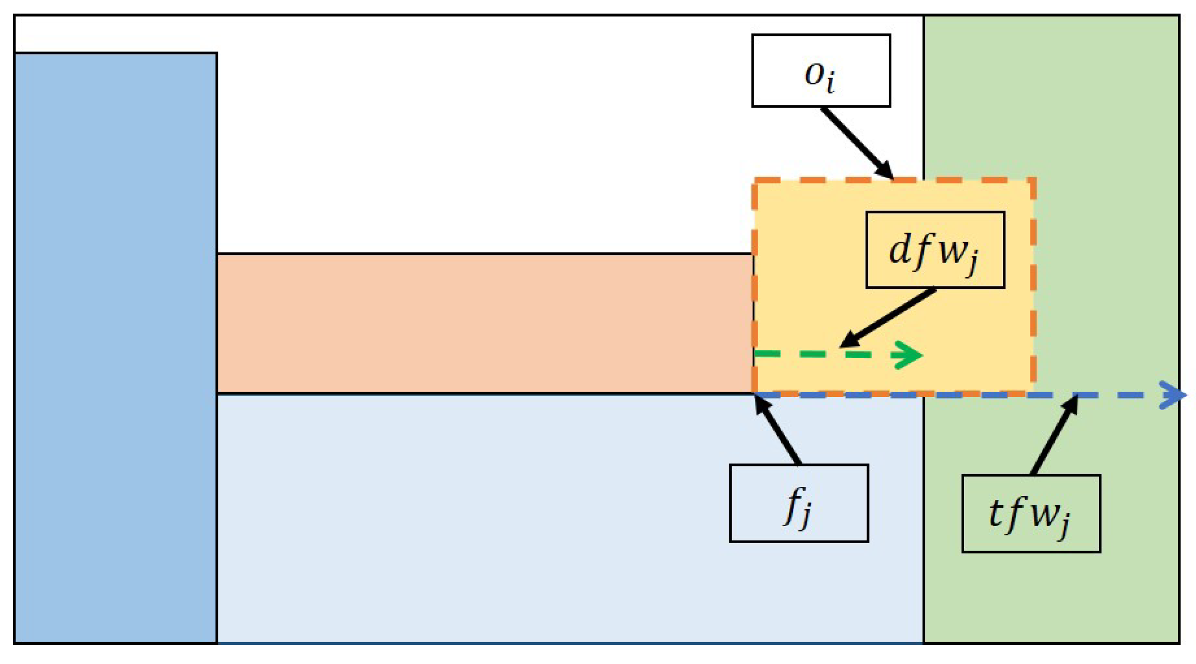
Figure 1 shows the characteristics of the flags and the objects, i.e.,
and
are the flag’s desirable and total width, respectively;
and
are the height to the left and to the right of the flag. Finally,
is the starting point and
and
are the current object width and height, respectively.
The selection of the first object is the one with the largest area. We select the rest of the elements according to the waste area function which is similar in some sense to the feature selection used in [
28]; the
value stores all waste area values for each object for a specific flag. Additionally, we validate that
in line 12. Therefore, if no object fits in the space of the flag, then we try to raise the flag (see line 35 of Algorithm 3).
| Algorithm 3 GRASP Construction Part 2 |
- 30:
if then - 31:
- 32:
- 33:
end if - 34:
else - 35:
- 36:
end if - 37:
end while
|
Later, Equation (
8) calculates a limit value, which will be compared with the waste areas of the candidate objects to create the restricted candidate list (
).
where
is a real number between 0 and 1; we made several tests to identify the best value, but we could not find it; hence, we chose to use random values between 0.4 and 0.5, which were the values with the best performance.. Additionally, the objects have a wide variety of sizes and, therefore, wastes, meaning that there might be lower or higher differences among the wastes. Hence, we could end up without candidates or with a lot of them, nullifying the purpose of the restricted candidate list.
Therefore, the candidate list selects , which are either five elements or 10% of the objects in until exhaust (see line 13). As a result, the algorithm initializes the restricted candidate list with the elements in with the lowest waste.
Line 17 obtains the index of the object for which the waste is minimal. Then, we update the restricted candidate list () and the restricted waste list (), respectively (see lines 18, and 19). Finally, the procedure removes from W (see line 20).
The algorithm calculates the value to further restrict the to those wastes that have a lower or equal value than (see line 22). Therefore, the algorithm updates and in lines 25 and 26, respectively.
The procedure selects an object
in
randomly with a roulette technique [
29] (see line 29); for further explanation see
Section 3.2.


 ,
, 


