Vision-Guided Six-Legged Walking of Little Crabster Using a Kinect Sensor

Abstract

A conventional blind walking algorithm has low walking stability on uneven terrain because a robot cannot rapidly respond to height changes of the ground due to limited information from foot force sensors. In order to cope with rough terrain, it is essential to obtain 3D ground information. Therefore, this paper proposes a vision-guided six-legged walking algorithm for stable walking on uneven terrain. We obtained noise-filtered 3D ground information by using a Kinect sensor and experimentally derived coordinate transformation information between the Kinect sensor and robot body. While generating landing positions of the six feet from the predefined walking parameters, the proposed algorithm modifies the landing positions in terms of reliability and safety using the obtained 3D ground information. For continuous walking, we also propose a ground merging algorithm and successfully validate the performance of the proposed algorithms through walking experiments on a treadmill with obstacles.

1. Introduction

The 2011 nuclear power plant explosion in Fukushima, Japan, was the result of a powerful earthquake and massive tsunami. Because it was impossible for humans to perform clean-up and dismantling tasks in the nuclear power plant, military robots, T-hawks, and Packbots from the United States were dispatched to the power plant. However, they were not able to complete their missions due to uneven terrain, including slopes, stairs, and ladders. After this failure, the Defense Advanced Research Project Agency (DARPA) in 2012 launched a robotics challenge project requesting robots to perform tasks specified particularly for disaster circumstances, and Team ViGIR realized those tasks through computer simulations in 2013 [1]. Feng S. et al. generated walking paths considering the center of mass (CoM) and performed simulations and experiments of biped walking and ladder climbing using the humanoid robot ATLAS (Boston Dynamics Co., Boston, MA, USA) [2]. In 2014, Team KAIST implemented dynamic and static walking on the DRC-HUBO for rough terrain similar to that of disaster environments while applying a vision system to the DRC-HUBO for object recognition and gripping [3]. Huang Y. et al. generated a walking path and achieved stable walking on uneven terrain for a small six-legged robot with stereo cameras [4]. Likewise, numerous studies on locomotion and tasks in hazardous environments were actively performed.

Because most disaster environments include rough terrain, locomotion capability on rough terrain is essential for successful movement. Li T.H.S. et al. achieved stable walking on inclined slopes for aiRobot-V by measuring ZMP error and trunk inclination using foot force sensors and an accelerometer [5]. They proposed a dynamic balance controller that includes a Kalman filter and a fuzzy motion controller. Luo R.C. et al. proposed a biped-walking trajectory generator based on the three-mass angular momentum model using model predictive control. As a result, they were able to reduce both the modeling error and zero moment point horizon and modify walking patterns against unexpected obstacles [6]. In addition to biped walking robots, Roennau A.et al. developed six-legged walking of the LAURON V on uneven terrain by applying sensor data including currents and ground contacts to stance and swing behaviors [7].

As far as we have been able to investigate, most legged robots have used blind-walking methods, which modify foot landing position based on the measured foot force, without using a vision system. While blind-walking methods enable legged robots to walk on rough terrain, blind-walking is somewhat slow and leads to a high risk of the robot falling down when confronted with excessive height or slope changes. Moreover, if there is an obstacle higher than the foot swing height, the foot may collide with the obstacle, leading to a fatal malfunction for robot systems. In order to solve these problems of blind-walking, studies on obstacle avoidance using vision sensors during walking have been gradually conducted since 2000. Sridharan M. et al. obtained locations of a robot and a target object from landmarks attached to specific locations and multiple cameras attached to the external environment within the moving range [8]. They used the Monte Carlo algorithm to create a map and realize the location of the robot. Michel P. et al. proposed a vision-guided walking method that can calculate locations of obstacles for the humanoid robot ASIMO and generate a walking path while avoiding obstacles in real-time [9]. These studies have an advantage since their robots can easily obtain accurate obstacle locations by installing vision systems in the external environment and not directly onto the robot body. On the other hand, there is a disadvantage in that the locomotion range of the robot is restricted due to the limitations in the captured image of the area with the environment-fixed vision systems.

Recently, several walking methods for legged robots with vision systems were proposed to compensate for the aforementioned disadvantage. Thompson S. et al. used stereo vision to implement 2D localization of a humanoid robot, H7, and performed biped walking while avoiding obstacles on the walking path [10]. Chilian A. et al. developed a navigation algorithm for mobile robots in unknown rough terrain [11]. Solely relying on stereo images from robot-fixed cameras, the algorithm uses visual odometry for localization. The authors validated the concept with a wheeled robot and a six-legged robot. Belter D. et al. determined six DOF poses of a six-legged robot with a monocular vision system using the Parallel Tracking and Mapping (PTAM) algorithm and Inertial Measurement Unit (IMU). They used a self-localization system together with an RRT-based motion planner, which allows a robot to walk autonomously on unknown rough terrain [12]. Many researchers have studied vision system-based walking robots; however, the majority of studies were restricted to localization in generated maps and walking path planning for avoiding obstacles.

Furthermore, because those studies were mainly focused on obstacle avoidance and path planning, without considering the ground shape, they did not attempt to improve dynamic walking stability, which is typically defined as how stably the robot is able to walk at high walking speeds. More recently, an attempt was made to use ground shape information from a depth camera in online walking pattern generation. Bajracharya M. et al. developed a stereo vision near-field terrain mapping system for the Legged Squad Support System (LS3) to automatically adjust robot gait in complex natural terrain [13]. Ramos O.E. et al. proposed a method for stable biped walking on rough terrain using inverse dynamics control and stereo vision information [14]. They successfully implemented a stable 3D dynamic walking simulation by using the ground shape information obtained from a depth camera attached to the robot head. As the above works show, only a few studies of vision-guided walking algorithms for improving walking stability were experimentally performed [15,16]. While employing vision sensors and tactile sensors, these recent works did not consider the safety and reliability simultaneously in determining the landing positions [17,18].

In this paper, we developed a vision-guided walking algorithm for a real six-legged robot. The main contributions of this work are (1) a spatial noise-filtering method of 3D ground information using a cost-effective Kinect sensor, (2) a landing position determination algorithm considering safety and reliability, and (3) a ground merging algorithm between successive ground data using the overlapped area. The foot landing positions can be adjusted according to the ground shape information, which was obtained from a Kinect sensor. In addition, we achieved highly stable six-legged walking by applying a balance control algorithm previously developed by the author [19]. A newly-developed special calibration tool can help us to derive a coordinate transformation relationship between the camera coordinate system and the robot-fixed coordinate system. The proposed algorithm can adjust the foot landing position by considering the reliability and safety of the landing area by merging 3D ground shape data obtained from the Kinect sensor. We validate the proposed vision-guided six-legged walking algorithm through walking experiments of a six-legged robot, LCR 200.

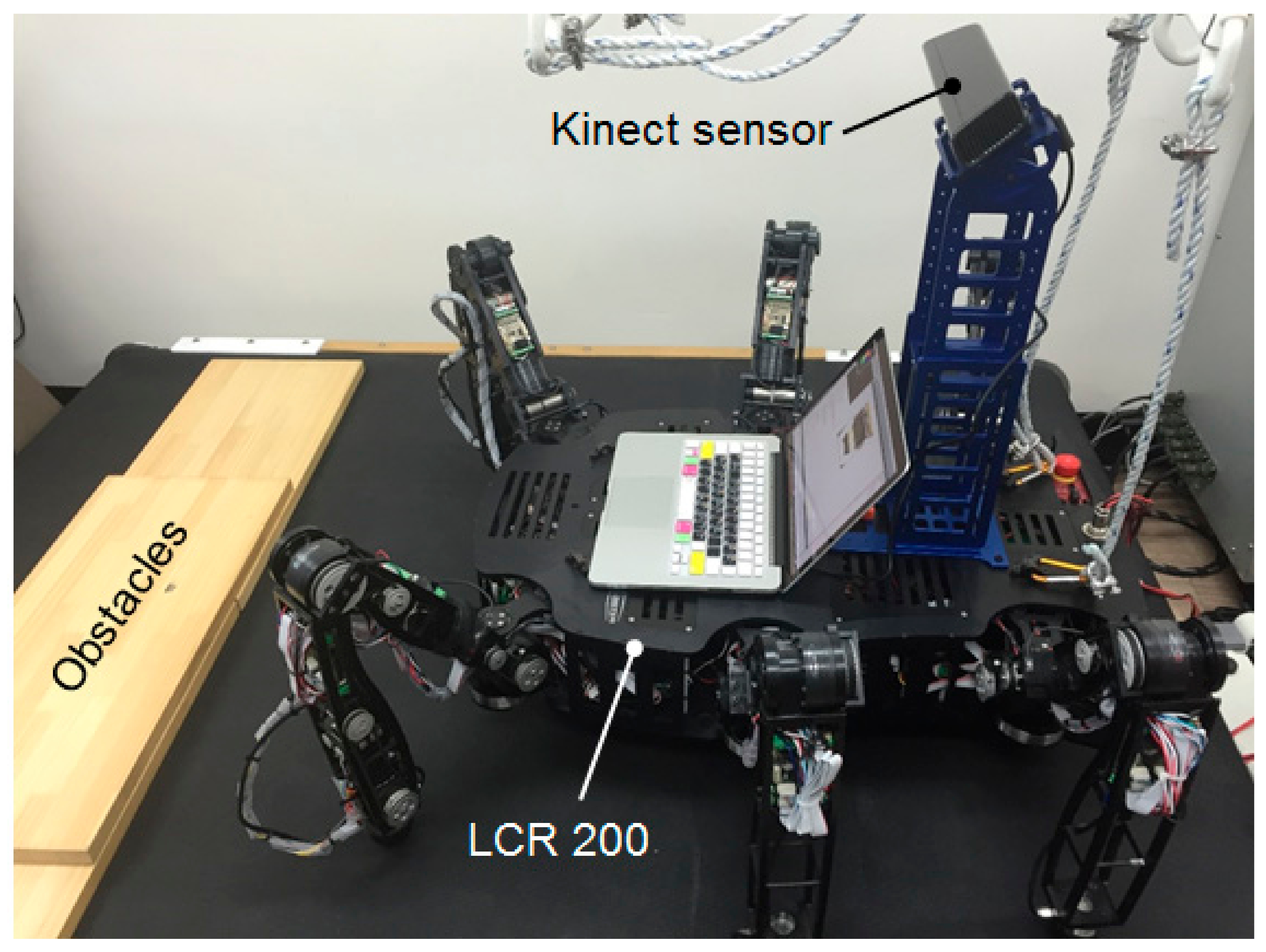
2. Little Crabster, LCR 200 with Kinect Sensor

Figure 1 shows the overall shape of LCR 200, which is a small-sized ground test platform of an underwater walking robot, Crabster [20]. The robot has six motor-driven legs with 30 DOFs for stable walking on uneven terrain. For motion control, the main control PC sends position commands to motor controllers at a frequency of 100 Hz while receiving information about the environment through various sensors. In particular, a Kinect sensor is employed for gathering the depth and RGB information of the environment and determining suitable landing positions on uneven ground. The Kinect sensor can be tilted in the pitch direction and moved vertically or longitudinally to adjust the field of view. In addition, load cells and F/T sensors are attached to each leg to control the center of pressure (CoP) and the foot compliance. An inertial sensor is also attached to the body center for posture control. Detailed specifications of LCR 200 are summarized in

Table 1. Specifications of LCR 200.

Specification	LCR 200
Dimensions	1000 (L) × 900 (W) × 500 (H) mm
Weight	54 kgf
DOF	30 (7 for front two legs, 4 for rear four legs)
Actuators	48 V Maxon BLDC motors with harmonic gears
Sensors	3-axis force/torque sensor at each hip 6-axis inertial sensor at body center. Compressive loadcell at each foot, Kinect sensor
Power supply	Li-Polymer battery (48 V, 360 Wh)
Operating system	Robot PC: Windows XP with RTX for robot body control Vision PC: Windows 7 for Kinect sensor
Motor servo controllers	2-Ch 200 W BL4804DID (Robocubetech Co., Seoul, Korea)
Control system	Distributed control system using CAN communication (control frequency: 100 HZ)

.

3. Camera–Robot Coordinate Transformation

3.1. Depth Camera—CCD Camera Calibration

The Kinect sensor, which is used to obtain ground information, consists of a depth camera for depth images and a CCD camera for color images. The two cameras have different fields of view and different locations; hence, a calibration tool was specially developed to match the purpose. The calibration tool was designed so that it can be firmly attached to the front of the robot, as shown in Figure 2a, and locations of the two target balls can be moved during the calibration process. The vertical movable range of the target balls starts from 20 mm to 360 mm, and the target balls can be rotated with respect to the central column at an interval of 45 degrees. In addition, considering that the highly reliable depth range of the Kinect sensor is approximately 0.8 m to 1.2 m, the central column can be moved 0.51 m to 0.57 m from the front of the robot. In order to distinguish the two target balls, different colors were applied. Figure 2b shows the calibration tool attached to the front of the robot LCR200.

As mentioned earlier, a matching process between RGB-color image and depth image is necessary. Using the OpenCV library, locations of the red and blue target balls of the calibration tool were obtained from color information in the color image (Figure 3a,b). Second, 3D coordinates of the target balls were also obtained, as shown in Figure 3c, from the depth image, and the two images were then matched using the locations of the two target balls and their distances in the two images. On the other hand, since the field of view and resolution of the depth image are smaller than those of the color image, the image size and resolution of the merged image was determined according to that of the depth image (320 × 240 pixels), as shown in Figure 3d. Through this merged image, it is possible to obtain the 3D coordinates of the arbitrarily selected point in the merged image.

3.2. Derivation of Transformation Matrix Using Tsai Algorithm

3.2.1. Image Acquisition

In order to obtain 3D coordinate information about the ground using a Kinect sensor, the 3D coordinates ($p_x, p_y, p_z)$ of the ground points can be calculated from 2D coordinates ($I_x, I_y)$ and depth values (d) of the merged image. Since the units of the 2D coordinates ($I_x, I_y)$ are pixel; the pixel unit has to be converted to the metric unit (mm) by using a scale factor. If the scale factor is constant, the coordinate error increases proportionally to the distance from the image center. This error is from that the distance between pixels increases according to the longitudinal and lateral distances between the object and the camera (see Figure 4a). In order to accurately obtain coordinates ($p_x, p_y, p_z)$, it is necessary to calculate the coordinates by considering the field of view (FOV) of the camera. Since the horizontal and vertical FOVs of the depth camera are 58.5 degrees and 46.6 degrees, respectively, and their horizontal and vertical pixel numbers are 320 and 240, respectively, the 3D coordinates can be obtained from the depth value d and the trigonometrical functions with rotation angles ${\theta }_1$ and ${\theta }_2$ of the merged image using Equation (1) (see Figure 4b).

$$\left\{\begin{array}{c}{p}_x=d·\cos {\theta }_1\cos {\theta }_2 \\ p_y=d·\cos {\theta }_1\sin {\theta }_2\\ p_z=d·\sin {\theta }_1\end{array}\right.$$

(1)

where

$$\left\{\begin{array}{c}{\theta }_1=\frac{{46.6}^{°}}{240pixel}{I}_y\\ {\theta }_2=\frac{{58.5}^{°}}{320pixel}{I}_x\end{array}\right.$$

3.2.2. Coordinate Transformation

In order to use the obtained 3D coordinates for the robot’s walking, it is first necessary to calculate a homogeneous transformation matrix between the robot-fixed coordinate frame and the camera-fixed coordinate frame; the homogeneous transformation matrix was then derived using the Tsai algorithm [21]. Figure 5a shows the experimental setup for this process. First, homogeneous transformation matrices A₁ and A₂, which indicate the relationships of the two different camera positions to a known target ball position, were derived. Second, homogeneous transformation matrices B₁ and B₂ from the robot-fixed coordinate frame to the two camera holder positions were obtained from the CAD information. Finally, a homogeneous transformation matrix X, which shows the relationship between the camera holder position and the Kinect camera, was derived using the A and B matrices indicated in Figure 5a, and a homogeneous transformation between the robot-fixed coordinate frame and the camera-fixed coordinate frame was obtained.

More specifically, we collected 3D coordinates of the many target ball positions with respect to both the camera-fixed coordinate and the robot-fixed coordinate frames for two different Kinect sensor positions, as shown in Figure 5b. The target ball positions were accurately changed using the developed calibration tool. In contrast to the conventional Tsai algorithm, optimized matrices A₁ and A₂ were derived from the pseudo inverse of Equations (2) and (3). In Equations (2) and (3), D_1i and D_2i are the two 3D camera-fixed coordinates of n positions of the target ball for two different camera positions, and the values of P_i are the known robot-fixed coordinates of n positions of the target ball.

$$A_1{D}_1=P; A_1\left[\begin{array}{cccc}{D}_{11x}& D_{12x}& \cdots & D_{1nx}\\ D_{11y}& D_{12y}& \cdots & D_{1ny}\\ D_{11z}& D_{12z}& \cdots & D_{1nz}\\ 1& 1& 1& 1\end{array}\right]=\left[\begin{array}{cccc}{P}_{1x}& P_{2x}& \cdots & P_{nx}\\ P_{1y}& P_{2y}& \cdots & P_{ny}\\ P_{1z}& P_{2z}& \cdots & P_{nz}\\ 1& 1& \cdots & 1\end{array}\right]$$

(2)

$$A_2{D}_2=P; A_2\left[\begin{array}{cccc}{D}_{21x}& D_{22x}& \cdots & D_{2nx}\\ D_{21y}& D_{22y}& \cdots & D_{2ny}\\ D_{21z}& D_{22z}& \cdots & D_{2nz}\\ 1& 1& 1& 1\end{array}\right]=\left[\begin{array}{cccc}{P}_{1x}& P_{2x}& \cdots & P_{nx}\\ P_{1y}& P_{2y}& \cdots & P_{ny}\\ P_{1z}& P_{2z}& \cdots & P_{nz}\\ 1& 1& \cdots & 1\end{array}\right]$$

(3)

Matrix A was then calculated from matrices A₁ and A₂, as in Equation (4), and matrix B was also calculated from matrices B₁ and B₂, as in Equation (5) in the same manner.

$$A=A_1{A}_2{}^{-1}=\left[\begin{array}{cccc}1.08& -0.15& 0.02& 2.69\\ -0.08& 0.98& -0.07& 77.54\\ -0.10& -0.09& 1.05& 0.60\\ 0& 0& 0& 1\end{array}\right]$$

(4)

where $A_1=\left(P{D}_1^T\right){\left(D_1{D}_1^T\right)}^{-1}, A_2=\left(P{D}_2^T\right){\left(D_2{D}_2^T\right)}^{-1}$

$$B=B_1{}^{-1}{B}_2=\left[\begin{array}{cccc}1.00& 0.00& 0.00& -100.00\\ 0.00& 1.00& 0.00& 0.00\\ 0.00& 0.00& 1.00& 50.00\\ 0& 0& 0& 1\end{array}\right]$$

(5)

In Figure 5a, the relationship among matrices A, B, and X can be derived as in Equation (6), and matrix X was finally calculated as in Equation (7) by solving the relationship expressed in Equation (6).

$$XA=BX$$

(6)

$$X=\left[\begin{array}{cccc}0.75& 0.02& 0.66& -125.43\\ 0.02& 1.00& -0.05& -15.03\\ -0.66& 0.05& 0.75& 94.88\\ 0& 0& 0& 1\end{array}\right]$$

(7)

Consequently, the homogeneous transformation matrix $T_C^R$ between the robot-fixed coordinate frame and the camera-fixed coordinate frame was calculated as in Equation (9) by using the obtained matrix X and a homogeneous transformation matrix T₁ in Equation (8) between the robot-fixed coordinate frame and the camera holder fixed coordinate frame, as shown in Figure 6.

$$T_1=\left[\begin{array}{cccc}1.00& 0.00& 0.00& 140.00\\ 0.00& 1.00& 0.00& 0.00\\ 0.00& 0.00& 1.00& 618.00\\ 0& 0& 0& 1\end{array}\right]$$

(8)

$$T_C^R=T_1·X=\left[\begin{array}{cccc}0.75& 0.03& 0.66& 14.57\\ 0.02& 1.00& -0.05& -15.03\\ -0.66& 0.05& 0.75& 712.88\\ 0& 0& 0& 1\end{array}\right]$$

(9)

3.2.3. Error Evaluation

We performed coordinate transformation experiments to verify the position accuracy of the proposed algorithm by comparing the actual position data of the target balls to the calculated position data of the target balls using a Kinect sensor.

Table 2. Results of coordinate transformation.

Camera-Fixed Coord. (mm)			Actual Robot-Fixed Coord. (mm)			Calculated Robot-Fixed Coord. (mm)			Error (mm)
X	Y	Z	X	Y	Z	X	Y	Z	X	Y	Z
1168.92	211.39	455.32	1200.00	200.00	300.00	1198.11	196.97	293.45	1.89	3.03	6.55
1189.03	−191.32	449.28	1200.00	−200.00	250.00	1197.13	−205.03	255.51	2.87	5.03	5.51
1017.83	12.58	339.53	1000.00	0.00	300.00	1002.41	0.93	296.39	2.41	0.93	3.61
1343.23	11.99	567.23	1400.00	0.00	250.00	1696.72	−4.54	252.37	3.28	4.54	2.37
1057.88	159.83	372.49	1068.40	141.40	300.00	1058.62	147.33	302.04	9.98	5.93	2.06
1304.08	−128.39	549.29	1341.40	−141.40	250.00	1351.31	−144.80	257.74	9.91	3.40	7.74
1059.32	−129.58	398.53	1068.60	−141.40	300.00	1068.20	−143.35	306.15	0.40	1.95	6.15
1295.87	159.99	519.23	1341.40	141.40	250.00	1333.96	144.92	255.03	7.44	3.52	5.03
1262.80	−123.11	571.88	1341.40	−141.40	300.00	1335.42	−141.48	302.19	5.98	0.08	2.19
1101.85	153.52	332.01	1068.60	141.40	250.00	1064.69	143.93	242.43	3.91	2.53	7.66
1279.34	153.20	559.23	1341.40	141.40	300.00	1347.76	135.80	295.60	6.36	5.60	4.40
1106.23	−139.76	361.39	1068.60	−141.40	250.00	1078.57	−150.73	246.82	9.97	9.33	3.18
								Max	9.98	9.33	7.74
								Avg	6.28	4.51	5.10

shows the coordinates of the target ball in the camera-fixed coordinate frame, the actual coordinates of them in the robot-fixed coordinate frame, and the calculated coordinates of them in the robot-fixed coordinate frame. As a result, the maximum error in each axis between the actual coordinate and the calculated coordinate was less than 10 mm, and the averaged errors were 6.28 mm, 4.51 mm, and 5.10 mm for the X, Y, and Z axes, respectively. These averaged values are sufficiently small to allow good recognition of the terrain condition. Since our robot can blindly walk on the uneven terrains compensating max. 10 mm height deviation, this error range (max 9.98 mm) in Table 2 did not show any negative effect on the proposed walking algorithm.

3.3. Image Post-Processing

Image post-processing was additionally conducted to enhance the accuracy and reliability of the 3D ground data because the initial 3D ground data obtained from the Tsai algorithm included noise and vertical ground offset between the robot-fixed coordinate frame and the ground. First, the vertical ground offset was experimentally measured when the robot was placed on flat level ground in a walking-ready posture. More specifically, the initial 3D ground data on the flat level ground were captured and saved, and then the 3D ground data with respect to the ground level were obtained by subtracting the initially saved 3D ground data from the measured 3D ground data. Figure 7 provides a comparison of 3D ground data with or without vertical ground offset. Through the processes above, more reliable 3D ground data with respect to ground level were obtained, as shown in Figure 7b.

Second, even after the ground offset is eliminated, when the 3D ground data are obtained from a Kinect sensor, noises can occur due to external light sources and irregular reflections, as shown in Figure 8a. In order to remove the noise with a high rate of change and to preserve the object’s edges with a low rate of change, filtering of the 3D ground data was performed using a 1st spatial low-pass filter. As shown in Figure 8c, spatial low-pass filtering in the x and y directions is applied sequentially to the obtained image according to Equations (10) and (11).

$$H_{\left(x,y+1\right)}=H_{\left(x,y\right)}+a\left(Z_{\left(x,y+1\right)}-H_{\left(x,y\right)}\right)$$

(10)

$$H_{\left(x+1,y\right)}=H_{\left(x,y\right)}+a\left(Z_{\left(x+1,y\right)}-H_{\left(x,y\right)}\right)$$

(11)

In the equations, H is the filtered depth, Z is the original depth, and a is the smoothing factor. The factor a was experimentally determined to remove the noises and preserve the object edges. If the smoothing factor is close to 1, the filtering effect becomes minimal. However, if the smoothing factor is close to 0, the filtering effect becomes maximum, and thus original depth is neglected. Based on the rigorous experiments, we finally determined the smoothing factor as 0.92. Finally, the smoothened ground image using the spatial low-pass filter was derived as Figure 8b. In order to confirm the performance of the spatial low-pass filtering, the RMS error value for the ground height was calculated, and the results confirmed a significant reduction in RMS error by 43.4 percent (from 3.3 mm to 1.87 mm). Finally, a linear interpolation method was used to determine the ground height between the data points because the distance between two data points of the obtained 3D ground data is approximately 4.4 mm at 1.1 m in front of the Kinect sensor. These three post-processes were performed to obtain accurate and stable 3D ground data.

4. Vision-Guided Walking Algorithm

4.1. Wave Gait Pattern Generation

Figure 9 shows the vision-guided walking algorithm framework of the LCR 200, using the independent joint position control method. When a standard walking pattern for the level ground is implemented, foot landing positions are modified according to the ground information from the vision system, which subsequently modifies the position trajectories of the six feet. Modified foot position trajectories are transformed to joint angle trajectories through inverse kinematics, and PD servo controllers then control the joint angles independently. Additionally, foot position trajectories are modified by the balance control unit using sensor feedback data [17].

First, by assuming that the ground is completely level, it is necessary for the robot to generate a standard walking pattern. In this study, we chose the wave-typed walking pattern shown in Figure 10, which has the highest walking stability on rough terrain. In order to generate a suitable standard walking pattern, nine walking parameters were introduced, as described in

Table 3. Nine walking pattern parameters.

Walking Parameters	Description
(1) Swing Time (Tsw)	Time duration of foot in air
(2) Delay Time (Td)	Time interval between foot landing and swing = Delay Ratio (κd) × Tsw
(3) Step Time (Tst)	Tst = Tsw + Td
(4) Walking Cycle Time (Twc)	Twc = 6 × Tst
(5) Swing Height (Hsw)	Maximum foot swing height
(6) Body Height (Hb)	Averaged body height from the six feet
(7) Step Length (Ls)	Longitudinal step length
(8) Side Step Length (Lss)	Lateral step length
(9) Rotation Angle (BCθ)	Body rotational angle

[22]. The introduced walking parameters are changeable during walking, except for the step time, and trajectories are generated simply using the several profile functions, which consist of sinusoidal functions. Figure 11 shows an example of a walking pattern. Figure 11a,b denote relative foot position trajectories from the initial ground positions in X- and Z-directions. It can be seen that step length and swing height change during walking. Therefore, it is possible to change the foot positions with ease during walking.

4.2. Landing Position Modification Algorithm

The walking pattern introduced in Section 4.1 is for the level ground without considering changes in the ground height. Hence, in order to increase the walking stability, it is necessary to adjust foot landing positions through ground information obtained by the vision system. For example, when our robot lands a foot on an obstacle, not on level ground, we have to modify the landing height from the ground information in advance. Furthermore, if the foot lands at the edge of an obstacle, the landing foot can slip on the edge and cause the LCR 200 to fall down; hence, the horizontal landing position must also be modified. For this reason, we propose an algorithm that modifies the landing positions by deciding on the reliability of the depth information and the safety of the landing area. Figure 12 shows a flow chart of the algorithm. First, the vision PC receives the scheduled foot landing position data from the robot PC. Second, the reliability of the depth data at each given landing area is checked. Third, the safety of each given landing area is also checked. If both reliability and safety are verified for the original landing area, the original horizontal position and corresponding vertical ground height are sent back to the robot PC. If the reliability or safety is not verified, the eight alternative landing positions around the original landing position are considered (see Figure 13). In case there is no safe landing area among the alternative landing positions, the safest position among them is selected alternatively. In the worst-case scenario, where all alternative positions are not reliable nor safe, the original landing position with zero vertical ground height is sent back to the robot PC for blind stepping.

To check the reliability of the depth information, we used the collection rate of the depth data in the landing area, which is 30 mm × 30 mm square around the landing position. Basically, if the collection rate of the landing area is moderate, as shown in Figure 14a, the depth data would be reliable, whereas if the collection rate is low due to a low data-concentrated section in the landing area, as illustrated in Figure 14b, the reliability would not be secured. It should be noted that if the high data-concentrated section and low data-concentrated section exist together, the collection rate of the landing area can be suitable, even though this landing area is not suitable for foot landing. In order to solve this problem, we divided the landing area into 100 sub-cells, as illustrated in Figure 15, and calculated the collection rate by checking whether a depth value exists or not in each sub-cell. By using this method, the reliability of the depth information of the landing area can be more suitably determined. The 30 mm × 30 mm landing area around the landing position is divided into 100 cells, and if the number of the cells containing the depth data is higher than 70%, we can decide that the reliability of the corresponding landing position is secured.

Next, to check the safety of the landing area, we consider the degree of ground height change. More specifically, we calculated the standard deviation of ground height in the landing area first and determined the safety by comparing the standard deviation with a predefined threshold. If the standard deviation is higher than the threshold at the landing area, the corresponding landing position is not appropriate for a stable landing. The threshold was determined by considering the edge of a 20 mm-thick block. A thickness of 20 mm was chosen because LCR 200 is able to blindly walk on a maximum of 20 mm-thick obstacles without a vision system. In Figure 16, it can be seen that when sudden height change is 20 mm, the standard deviation of the ground height in the landing area is theoretically 10 mm. Therefore, the landing position is assumed to be safe in cases in which the standard deviation of the ground height is less than 8 mm, considering a margin of 20%.

4.3. Ground Merging Algorithm

If the depth information for the 3D ground data is continuously received from the vision PC during walking, the computing burden of the robot PC becomes very high, and the accuracy of the depth information may decrease due to vibration transmitted to the Kinect sensor. For this reason, we periodically stopped the robot and scanned the uneven ground in a static state. For this strategy, it is necessary to merge the 3D ground data sets at every scanning. In the ground merging algorithm, there are two basic requirements, which are to make the robot level by using the body posture control and generate an overlapped area between current ground data and previous ground data, as illustrated in Figure 17. In addition, we assume that the displacement of the robot, kinematically calculated from the walking cycles, is the same as the actual displacement without any slip. With these requirements and assumptions, 3D ground data are merged using the information of the overlapped area.

Figure 18 shows a flowchart for the ground merging algorithm. First, 3D ground data with respect to the global coordinate frame is generated by scanning the ground and considering both the ground height and robot body height. For ground merging, ten sampled areas (size of each area is 10 mm × 10 mm) in the overlapped area, and the averaged ground heights of the previous 3D ground data and the current 3D ground data are then calculated, as shown in Figure 19. Consequently, averaged vertical ground offset is calculated by comparing the averaged ground heights; the result is applied to the current 3D ground data to merge the current 3D ground data with the previous data.

5. Experiment

In order to verify the proposed landing position modification algorithm, we placed 25 mm-thick obstacles on a treadmill and conducted walking experiments using the LCR 200 [23]. First, as shown in Figure 20, the LCR 200 tried to land the swing leg on the obstacle’s rear edge; this process had low reliability because the depth information at the back of the edge was unavailable due to an occlusion. Without the proposed algorithm, the landed foot slipped on the edge and dropped to the ground after landing, as shown in Figure 20a. On the other hand, when the proposed algorithm was applied to the robot, the landing position was modified from the rear edge to the stable surface, and the swing leg landed on the obstacle stably, as shown in Figure 20b.

Table 4. Depth data collection rate and standard deviation of ground height. (Reliability algorithm test).

	X (mm)	Y (mm)	Z (mm)	Depth Data Collection Rate	Standard Deviation (mm)
Original landing position	1036.35	−336.35	45.12	57%	13.14
1st Alternative landing position	1066.35	−336.35	8.37	71%	6.35
2nd Alternative landing position	1057.56	−315.14	10.36	54%	17.32
3rd Alternative landing position	1057.56	−357.56	11.97	63%	7.84
4th Alternative landing position	1036.35	−306.35	45.21	63%	11.97
5th Alternative landing position	1036.35	−366.35	45.33	58%	13.29
6th Alternative landing position	1015.14	−315.14	44.84	87%	4.23
7th Alternative landing position	1015.14	−357.56	44.89	81%	2.19
8th Alternative landing position	1006.35	−336.35	44.97	79%	5.57

shows the depth data collection rate and standard deviation of the ground height for the original landing position and eight alternative landing positions. It can be seen that the data collection rate of the original landing position was 57 %, which is less than the 70 % threshold. Hence, the robot sequentially searched for alternative eight landing positions and evaluated their reliabilities of them. Among alternative landing positions, the 1st, 6th, 7th, and 8th landing positions have reliabilities higher than the 70% threshold, and the robot chose the 6th alternative landing position, which has the highest reliability. Moreover, the chosen alternative landing position is sufficiently safe because the standard deviation of the ground height is much less than 8 mm.

Second, to test for a safe landing, we intentionally made the LCR 200 land the swing foot on the obstacle’s front edge, which has low safety due to the sharp edge, as shown in Figure 21. It can be seen in Figure 21a that, without the proposed algorithm, the landed foot also slipped on the obstacle and dropped to the ground, whereas the robot landed the swing foot on the safe area when using the proposed algorithm, as shown in Figure 21b.

Table 5. Depth data collection rate and standard deviation of ground height. (Safety algorithm test).

	X (mm)	Y (mm)	Z (mm)	Depth Data Collection Rate	Standard Deviation (mm)
Original landing position	936.35	−336.35	42.74	81%	17.64
1st Alternative landing position	966.35	−336.35	43.94	76%	5.67
2nd Alternative landing position	957.56	−315.14	42.31	67%	6.33
3rd Alternative landing position	957.56	−357.56	44.31	81%	6.18
4th Alternative landing position	936.35	−306.35	39.97	68%	10.92
5th Alternative landing position	936.35	−366.35	44.04	75%	11.24
6th Alternative landing position	915.14	−315.14	31.75	78%	11.84
7th Alternative landing position	915.14	−357.56	29.36	73%	14.49
8th Alternative landing position	906.35	−336.35	28.94	71%	13.61

shows the standard deviations of the ground height for the original and eight alternative positions. The original landing position has a standard deviation of 17.64 mm, which is higher than the 8 mm threshold; hence, the robot determined the original landing position as an unsafe position. Consequently, the robot searched for eight alternative positions and chose the 1st alternative landing position, which has the smallest standard deviation of 5.67 mm among eight alternative positions. Moreover, the 1st alternative position has reliability sufficiently higher than 70%.

In order to verify the performance of the vision-guided walking algorithm, we conducted a walking experiment with the LCR 200 on a large treadmill with obstacles [23]. Thirty millimeter-thick wood plates were used as obstacles; they were placed in a series of zigzags. As for the walking parameters, the step length was 100 mm, the swing time was 1 s, and the overlap time between steps was 0.3 s. Five ground scannings were performed, and three periods of walking (18 steps) were conducted at every scanning. Figure 22 shows snapshots of the ground scanning. The obstacles were additionally placed on the treadmill before each ground scanning. As a result, a merged 3D ground image was obtained, as shown in Figure 23, after the five ground scannings and mergings. The ground data were successfully merged, and the four ground obstacles were displayed clearly.

Table 6. Original and modified landing positions with depth data collection rates and standard deviations.

	Original					Modified
	X (mm)	Y (mm)	Z (mm)	Collection Rate (%)	SD (mm)	X (mm)	Y (mm)	Z (mm)	Collection Rate (%)	SD (mm)
3rd Scanning	1536.35	−336.35	47.50	99	3.33
	1100.00	442.83	40.52	53	4.57	1078.79	421.62	39.05	73	2.09
	800.00	−392.82	29.74	94	12.46	830.00	−392.83	41.67	97	1.81
	1636.35	336.35	3.00	97	2.01
	1200.00	−442.82	1.57	48	8.13	1200.00	−412.83	2.12	74	2.65
	900.00	392.83	0.05	97	2.27
	1736.35	−336.35	3.14	98	2.09
	1300.00	442.83	1.95	38	1.48	1330.00	442.83	2.04	76	2.7
	1000.00	−392.83	44.23	81	3.25
	1836.35	336.35	39.87	95	2.22
	1400.00	−442.83	40.45	38	4.65	1421.21	−421.62	42.61	79	2.25
	1100.00	392.83	39.49	86	2.14
	1936.35	−336.35	4.02	94	1.75
	1500.00	442.83	3.49	87	2.37
	1200.00	−392.83	1.62	94	2.55
	1936.35	336.35	40.80	96	3.43
	1500.00	−442.83	44.24	85	2.65
	1200.00	392.83	39.85	100	1.93
4th Scanning	2036.00	−336.35	3.48	86	1.82
	1600.00	442.83	2.57	51	8.22	1621.21	421.62	1.66	74	2.73
	1300.00	−392.83	5.46	97	11.41	1275.79	−371.62	0.80	97	1.99
	2136.35	336.35	3.12	97	2.24
	1700.00	−442.83	2.49	47	9.15	1721.21	−421.62	3.69	72	2.86
	1400.00	392.83	2.82	100	1.91
	2236.35	−336.35	3.30	99	1.70
	1800.00	42.83	38.80	75	3.04
	1500.00	−392.83	45.27	68	2.68
	2336.35	336.35	4.25	100	2.29
	1900.00	−442.83	1.45	56	1.56	1921.21	−421.62	1.18	80	1.81
	1600.00	392.83	392.00	71	2.31
	2436.35	−336.35	4.94	92	2.10
	2000.00	442.83	0.05	28	0.01	2000.00	442.83	0.00	53	2.91
	1700.00	−392.83	3.44	98	2.59
	2436.35	336.35	3.74	97	1.99
	2000.00	−442.83	0.15	58	0.83	2030.00	−442.83	1.05	72	2.26
	1700.00	392.83	34.24	97	17.48	1730.00	392.83	31.42	100	15.87
5th Scanning	2536.35	−336.30	4.97	82	2.63
	2100.00	442.83	1.22	54	1.57	2121.21	421.62	1.70	71	2.42
	1800.00	−392.83	2.05	100	1.72
	2636.35	336.35	−1.28	99	2.88
	2200.00	−442.83	2.90	73	2.40
	1900.00	392.83	40.05	89	1.80
	2736.35	−336.35	−2.68	97	3.29
	2300.00	442.83	3.78	30	6.24	2300.00	421.83	4.40	71	2.25
	2000.00	−392.83	2.28	82	2.34
	2936.35	336.35	−3.76	97	2.44
	2400.00	−442.83	2.63	95	1.86
	2100.00	392.83	1.36	71	2.51
	2936.35	−336.35	−2.63	97	2.37
	2500.00	442.83	4.86	91	2.16
	2200.00	−392.83	3.19	94	1.85
	2936.35	336.35	−3.46	97	2.12
	2500.00	−442.83	3.73	78	2.25
	2200.00	392.83	3.94	97	2.71

represents the reliabilities and safeties of the original and modified landing positions of the 3rd to 5th scannings. When both the reliability and safety were secured at the original landing position, the robot did not search for a modified landing position; hence, the modified landing positions indicated by the white lines in Table 6 became empty. In addition, in Table 6 the 1st and 2nd scannings were deleted because there was no modification of the original landing positions during those scannings. The 12 green lines show that the original landing positions with low reliability or low safety were modified to the most reliable and the safest positions among the eight alternative positions. All the collection rates and standard deviations of the modified landing positions are higher than 70% and lower than 8 mm, respectively. In the case of the first yellow line in the 4th scanning, the original landing position with zero height was determined because there was no reliable alternative landing position higher than 70%. In the case of the second yellow line in the 4th scanning, there was no safe alternative landing position; hence, among the reliable landing positions, the safest landing position with a standard deviation of 15.87 mm was chosen. Consequently, the LCR200 with the Kinect sensor was able to pass through the obstacles effectively by using the proposed algorithm. Figure 24 shows snapshots of the three cycles of walking after the 3rd scanning.

6. Conclusions

This paper proposed a vision-guided walking algorithm for a six-legged robot, LCR200, using a Kinect sensor for stable walking on uneven terrain. We developed a special calibration device and experimentally derived a transformation matrix between the camera-fixed coordinate frame and the robot-fixed coordinate frame using the Tsai algorithm with the Pseudo inverse optimization method. Three-dimensional ground data with respect to the robot-fixed coordinate frame were derived, and image post-processing was conducted in order to eliminate noise and derive 3D ground data at the ground level. In addition, we proposed landing position modification and ground merging algorithms to secure the reliability and safety of walking on uneven terrain. The proposed algorithm was successfully verified through a walking experiment using the LCR200 on a treadmill with obstacles.

The current study is limited to restricted environments because the Kinect sensor was designed for indoors: its resolution is relatively low, and significant noise is included in the depth data. Furthermore, we could not measure the 3D environment continuously since the shaking motion of the legged robot during fast dynamic walking often resulted in degraded accuracy of the measurements. In the near future, we will use a high resolution-depth sensor that can be used outdoors for more accurate landing position information. In this paper, the original landing positions, which were basically determined from the prescribed standard walking pattern, were modified within a given limited range. In future work, we also aim to develop an advanced step planning algorithm using optimization techniques or machine learning methods without the prescribed standard walking pattern for the given ground data.

After sufficiently evaluating the vision-guided walking algorithm for LCR 200, we plan to apply the same algorithm to Crabster, which is a six-legged underwater walking robot. The proposed algorithm will be easily adopted since Crabster has ultrasonic cameras, which can gather depth information in the underwater environment, and CCD cameras for color images.

References

1. Kohlbrecher, S.; Conner, D.C.; Romay, A.; Bacim, F.; Bowman, D.A.; von Stryk, O. Overview of team vigir’s approach to the virtual robotics challenge. In Proceedings of the IEEE International Symposium on Safety, Security, and Rescue Robotics (SSRR), Linkoping, Sweden, 21–26 October 2013; pp. 1–2. [Google Scholar]
2. Feng, S.; Whitman, E.; Xinjilefu, X.; Atkeson, C.G. Optimization-based full body control for the DARPA robotics challenge. J. Field Robot. 2015, 32, 293–312. [Google Scholar] [CrossRef] [Green Version]
3. Wang, H.; Zheng, Y.F.; Jun, Y.; Oh, P. DRC-Hubo walking on rough terrains. In Proceedings of the IEEE International Conference on Technologies for Practical Robot Applications (TePRA), Woburn, MA, USA, 14–15 April 2014; pp. 1–6. [Google Scholar]
4. Huang, Y.; Vanderborght, B.; Ham, R.V.; Wang, Q.; Damme, M.V.; Xie, G.; Lefeber, D. Step length and velocity control of a dynamic bipedal walking robot with adaptable compliant joints. IEEE/ASME Trans. Mechatron. 2013, 18, 598–611. [Google Scholar] [CrossRef]
5. Li, T.H.S.; Su, Y.T.; Liu, S.H.; Hu, J.J.; Chen, C.C. Dynamic balance control for biped robot walking using sensor fusion, kalman filter, and fuzzy logic. IEEE Trans. Ind. Electron. 2012, 59, 4394–4408. [Google Scholar] [CrossRef]
6. Luo, R.C.; Chen, C.C. Biped walking trajectory generator based on three-mass with angular momentum model using model predictive control. IEEE Trans. Ind. Electron. 2016, 63, 268–276. [Google Scholar] [CrossRef]
7. Roennau, A.; Heppner, G.; Nowicki, M.; Dillmann, R. LAURON V: A versatile six-legged walking robot with advanced maneuverability. In Proceedings of the IEEE/ASME International Conference on Advanced Intelligent Mechatronics (AIM), Besancon, France, 8–11 July 2014; pp. 82–87. [Google Scholar]
8. Sridharan, M.; Kuhlmann, G.; Stone, P. Practical vision-based monte carlo localization on a legged robot. In Proceedings of the IEEE International Conference on Robotics and Automation, Barcelona, Spain, 18–22 April 2005; pp. 3366–3371. [Google Scholar]
9. Michel, P.; Chestnutt, J.; Kuffner, J.; Kanade, T. Vision-guided humanoid footstep planning for dynamic environments. In Proceedings of the IEEE-RAS International Conference on Humanoid Robots, Tsukuba, Japan, 5–7 December 2005; pp. 13–18. [Google Scholar]
10. Thompson, S.; Kagami, S. Humanoid robot localisation using stereo vision. In Proceedings of the IEEE-RAS International Conference on Humanoid Robots, Tsukuba, Japan, 5–7 December 2005; pp. 19–25. [Google Scholar]
11. Chilian, A.; Hirschmüller, H. Stereo camera-based navigation of mobile robots on rough terrain. In Proceedings of the IEEE/RSJ International Conference on Intelligent Robots and Systems, St. Louis, MO, USA, 10–15 October 2009; pp. 4571–4576. [Google Scholar]
12. Belter, D.; Skrzypczynski, P. Precise self-localization of a walking robot on rough terrain using parallel tracking and mapping. Ind. Robot 2013, 40, 229–237. [Google Scholar] [CrossRef]
13. Bajracharya, M.; Ma, J.; Malchano, M.; Perkins, A.; Rizzi, A.A.; Matthies, L. High fidelity day/night stereo mapping with vegetation and negative obstacle detection for vision-in-the-loop walking. In Proceedings of the IEEE/RSJ International Conference on Intelligent Robots and Systems (IROS), Tokyo, Japan, 3–7 November 2013; pp. 3663–3670. [Google Scholar]
14. Ramos, O.E.; Garcia, M.; Mansard, N.; Stasse, O.; Hayet, J.B.; Soueres, P. Toward reactive vision-guided walking on rough terrain: An inverse-dynamics based approach. Int. J. Hum. Robot. 2014, 11, 1441004. [Google Scholar] [CrossRef]
15. Kanoulas, D.; Zhou, C.; Nguyen, A.; Kanoulas, G.; Caldwell, D.G.; Tsagarakis, N.G. Vision-based foothold contact reasoning using curved surface patches. In Proceedings of the IEEE-RAS 17th International Conference on Humanoid Robotics (Humanoids), Birmingham, UK, 15–17 November 2017; pp. 121–128. [Google Scholar]
16. Omori, Y.; Kojio, Y.; Ishikawa, T.; Kojima, K.; Sugai, F.; Kakiuchi, Y.; Okada, K.; Inaba, M. Autonomous safe locomotion system for bipedal robot applying vision and sole reaction force to footstep planning. In Proceedings of the IEEE/RSJ International Conference on Intelligent Robots and Systems (IROS), Macau SAR, China, 3–8 November 2019; pp. 4891–4898. [Google Scholar]
17. Xu, J.; Wu, X.; Li, R.; Wang, X. Obstacle Overcoming Gait Design for Quadruped Robot with Vision and Tactile Sensing Feedback. In Proceedings of the 4th International Conference on Robotics, Control and Automation Engineering (RCAE), Wuhan, China, 4–6 November 2021; pp. 272–277. [Google Scholar] [CrossRef]
18. Lee, M.; Kwon, Y.; Lee, S.; Choe, J.; Park, J.; Jeong, H.; Heo, Y.; Kim, M.S.; Sungho, J.; Yoon, S.E.; et al. Dynamic Humanoid Locomotion Over Rough Terrain With Streamlined Perception-Control Pipeline. In Proceedings of the 2021 IEEE/RSJ International Conference on Intelligent Robots and Systems (IROS), Prague, Czech Republic, 27 September–1 October 2021; pp. 4111–4117. [Google Scholar] [CrossRef]
19. Kim, J.Y. Dynamic balance control algorithm of a six-legged walking robot, little crabster. J. Intell. Robot. Syst. 2015, 18, 47–64. [Google Scholar] [CrossRef]
20. Kim, J.Y.; Jun, B.H. Design of six-legged walking robot, little crabster for underwater walking and operation. Adv. Robot. 2014, 28, 77–89. [Google Scholar] [CrossRef]
21. Tsai, R.Y. A versatile camera calibration technique for high-accuracy 3D machine vision metrology using off-the-shelf TV cameras and lenses. IEEE J. Robot. Autom. 1987, 3, 323–344. [Google Scholar] [CrossRef] [Green Version]
22. Kim, J.Y.; Jun, B.H.; Park, I.W. Six-legged walking of “Little Crabster” on uneven terrain. Int. J. Precis. Eng. Manuf. 2017, 18, 509–518. [Google Scholar] [CrossRef]
23. Kim, J.Y. Vision-Guided Six-Legged Walking of Little Crabster Using a Kinect Sensor. Available online: https://www.youtube.com/watch?time_continue=4&v=Svk6n43J4DE (accessed on 22 January 2022).
Figure 1. Photograph of LCR 200 with Kinect sensor.
Applsci 12 02140 g001
Figure 2. Calibration setup: (a) Developed camera calibration tool; (b) Photograph of LCR 200 with calibration tool.
Applsci 12 02140 g002
Figure 3. (a) Color image from Kinect sensor; (b) searched target balls in color image; (c) searched target balls in depth image; (d) merged image of color and depth images.
Applsci 12 02140 g003
Figure 4. Image acquisition: (a) Barrel distortion effect; (b) Calculation of the 3D coordinate of ground point.
Applsci 12 02140 g004
Figure 5. Coordinate transformation: (a) Experimental setup of Tsai algorithm; (b) Calculation of A1 and A2 matrices using pseudo inverse optimization.
Applsci 12 02140 g005
Figure 6. Final transformation matrix T C R between robot-fixed coordinate frame and camera-fixed coordinate frame.
Applsci 12 02140 g006
Figure 7. (a) Three-dimensional image of ground before eliminating ground offset; (b) after eliminating ground offset.
Applsci 12 02140 g007
Figure 8. (a) Three-dimensional ground image before applying spatial low-pass filtering; (b) after applying spatial low-pass filtering; (c) spatial low-pass filtering in x and y directions.
Applsci 12 02140 g008
Figure 9. Vision-guided walking algorithm framework of LCR 200 [19].
Applsci 12 02140 g009
Figure 10. Wave-typed walking pattern of six-legged robot [22] (L1: left first foot, L2: left second foot, L3: left third foot, R1: right first foot, R2: right second foot, R3: right third foot).
Applsci 12 02140 g010
Figure 11. Example of walking pattern generation of LCR 200 [22] (BC: body center): (a) X-trajectories of the six feet in ground-fixed coordinate frame; (b) Z-trajectories of the six feet in ground-fixed coordinate frame.
Applsci 12 02140 g011
Figure 12. Flow chart of landing position modification algorithm.
Applsci 12 02140 g012
Figure 13. Eight alternative foot landing positions and checking order.
Applsci 12 02140 g013
Figure 14. Depth data in landing area (red circle: low data concentration area, blue circle: high data concentration area, green circle: medium data concentration area): (a) moderate collection rated; (b) low collection rated; (c) moderate collection rated but unsuitable for foot landing.
Applsci 12 02140 g014
Figure 15. Reliability checking of cells in landing area.
Applsci 12 02140 g015
Figure 16. (a) Case of landing on unsafe edge; (b) case of landing on safe surface.
Applsci 12 02140 g016
Figure 17. Successive ground scanning areas and their overlapped area.
Applsci 12 02140 g017
Figure 18. Flowchart of ground merging algorithm.
Applsci 12 02140 g018
Figure 19. Scanned 3D ground data and calculation of averaged ground height from ten sampled areas within overlapped area. Blue box means a middle section of the ground data.
Applsci 12 02140 g019
Figure 20. Reliability algorithm test: (a) without proposed algorithm; (b) with proposed algorithm [23].
Applsci 12 02140 g020
Figure 21. Safety algorithm test: (a) without proposed algorithm; (b) with proposed algorithm [23].
Applsci 12 02140 g021
Figure 22. Snapshots of the five ground scannings [23].
Applsci 12 02140 g022
Figure 23. Merged 3D ground image after five ground scannings.
Applsci 12 02140 g023
Figure 24. Snapshots of three cycles of walking after 3rd scanning [23]. The number represents the sequence of snapshots during three cycles.
Applsci 12 02140 g024