2.6. Analytical Design of FOPI Controller for PCCS Combining with Smith Predictor
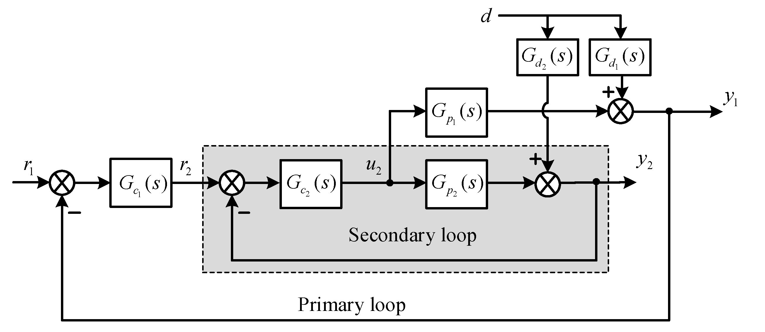
The general parallel cascade control system is shown in
Figure 2, where
and
are the transfer functions of the primary and secondary processes, respectively.
and
are the primary and secondary controllers;
is used to stabilize the primary control loop in case the transfer function
is kind of an unstable or integrating process.
and
denote the transfer functions of disturbances affecting the outputs.
denotes the equivalent closed-loop transfer function for servo response of the secondary loop (from the input
to the output
), and it can be calculated as follows:
Assuming that
(perfect model), Equation (13) becomes:
where
is the delay time at the primary output, and normally, it equals the delay time of the primary transfer function (
);
is the delay-free part of
.
In this work, the secondary process model is assumed as a well-known first order plus time delay process (FOPTD), as in Equation (15). The primary process model is investigated by one of the following transfer functions, as in Equations (16)–(18)
where Equation (17) represents the unstable first order plus time delay (UFOPTD) and Equation (18) is the second order integral plus time delay (SOIPTD).
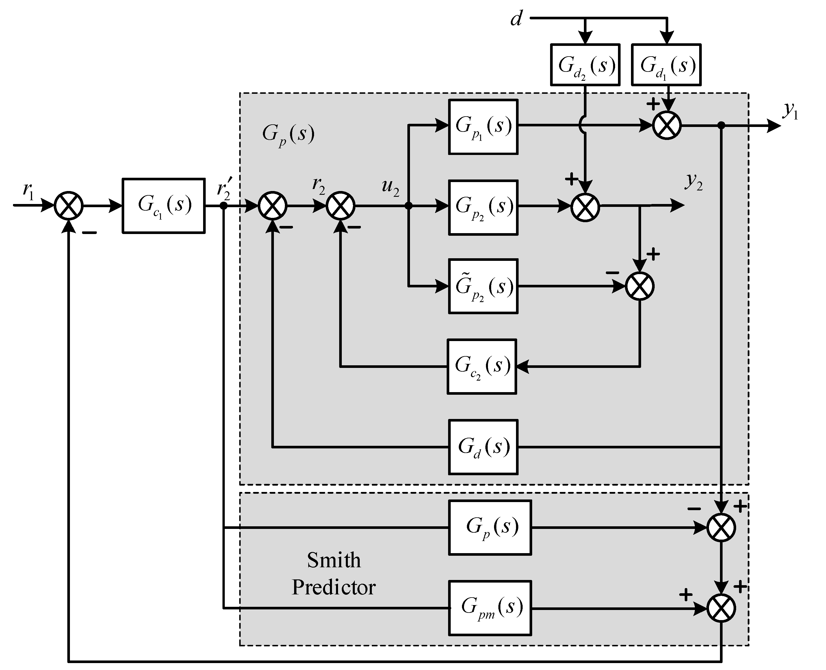
2.6.1. Design of Secondary Controller Based on IMC Approach for Disturbance Rejection
Figure 3 shows the block diagram of the secondary control design based on the IMC approach where
and
are the process and the process model respectively;
is the IMC controller. Note that, in this work, the IMC controller is placed on the feedback loop, which is different from the well-known IMC approach. As a result, the role of the controller is to solve the regulator problem in the secondary loop.
For the nominal case (
), the set-point and disturbance responses in
Figure 3 can be simplified as:
As mentioned above, the secondary transfer function
is stable in this study. Therefore, from Equation (19), it is obvious that the controller
is only used for disturbance rejection. The IMC approach [
27] is adopted to design
. The process model
is factored into two parts:
where
is the portion of the model which includes the dead time and/or right half plane zeros and
;
is the remaining portion of the secondary process. Therefore, we have:
To obtain a good disturbance rejection for the process
which has poles near zero at
, then
should have zeros at
. According to the IMC approach, the IMC controller is given as follows:
where
f is considered as the IMC filter whose transfer function is given in this case as follows:
Then the controller is obtained:
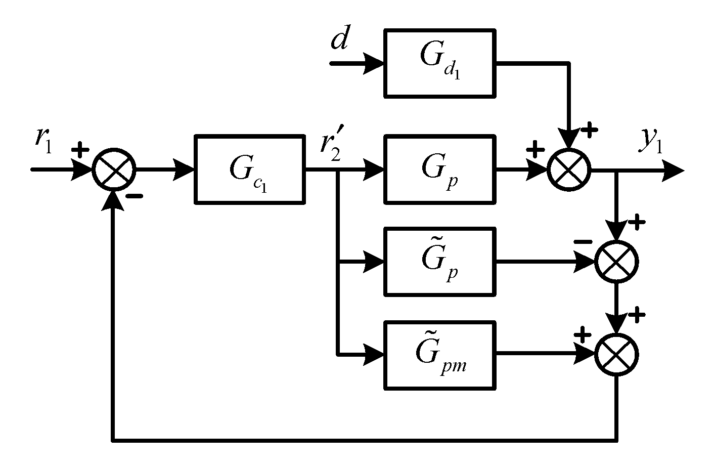
2.6.2. FOPI Controller Design for the Primary Control Loop
The block diagram of the system is reduced in
Figure 4 where
and
represent the equivalent process and the obtained transfer function from
to
in
Figure 2, respectively.
is
without the delay term. This structure follows the Smith predictor scheme to eliminate the sluggish response at the primary output when the primary process has a long delay time.
The closed loop transfer functions for the outer loop (from
r1 to
y1)
From Equation (25), it is obvious that the characteristic equation of the closed-loop system is the delay-free function. In order to design the primary controller, the equivalent process first has to be obtained. In this work, depending on the kinds of secondary process transfer functions, several methods are proposed to derive in the form of FOPTD.
Case 1: The primary process is FOPTD
The transfer function of the primary process is as Equation (16). In this case, the primary transfer function is also stable, so there is no need to use the stabilized controller,
, and from Equation (14):
Case 2: The primary process is UFOPTD
In this case, the primary process is unstable, hence, the stabilized controller is suggested as follows:
The equivalent transfer function is obtained:
Using Padé 1/1 approximation:
and choosing
where
,
and
.
To guarantee the stability criterion, two parameters
and
have to be greater than zero. Therefore, the parameter
has to meet the following requirement:
Case 3: The primary process is SOIPTD
The stabilized controller as in the previous case, Equation (28), is also needed in this case; therefore, the equivalent transfer function is derived as follows:
Similar to case 2, using Equation (30) to replace into Equation (34):
The condition of
is obtained:
Moreover, in this case,
is the second-order transfer function. To ensure a servo response of the closed-loop system, as well as to simplify the design problem, the system has to be the overdamped one which the damping factor has not to be less than 1. From Equation (35), another condition of
is also derived:
In that case, the system transfer function will be approximated to the first-order one. Applying the approximation technique using the PSO algorithm [
29], Equation (35) will be reduced to the first order plus time delay process as the two previous cases, Equations (26) and (31).
2.6.3. The General Proposed Design Method for the Above Three Cases of the Primary Controller
After deriving the equivalent transfer functions of primary processes in the three above cases to the general form of FOPTD, Equation (38), the proposed FOPI controller will be designed based on the IMC approach. However, the frequency domain mentioned above is addressed here.
In order to choose the fractional order of the controller, the relative dead time parameter is considered [
10]:
In this work, the fractional-order
is determined according to the value of
as Equation (40). It is based on the guideline in [
10], however, only the fractional order is considered in this study
Step 1: Design the stabilized controller
Case 1: The primary process transfer function is stable. Therefore, the stabilized loop will not be used in this case. Hence, is assigned to zero ()
Case 2: Note that when the order is greater than 1, system responses will create an overshoot. Therefore, in this work, to guarantee a good servo tracking of the primary control loop, the relative dead time parameter
will be chosen in the range of
, it means that
. From Equations (31) and (39), the following condition is obtained:
Case 3: For this case, the condition (36) and (37) are used to choose for the stabilized controller, remember that as in Equation (29).
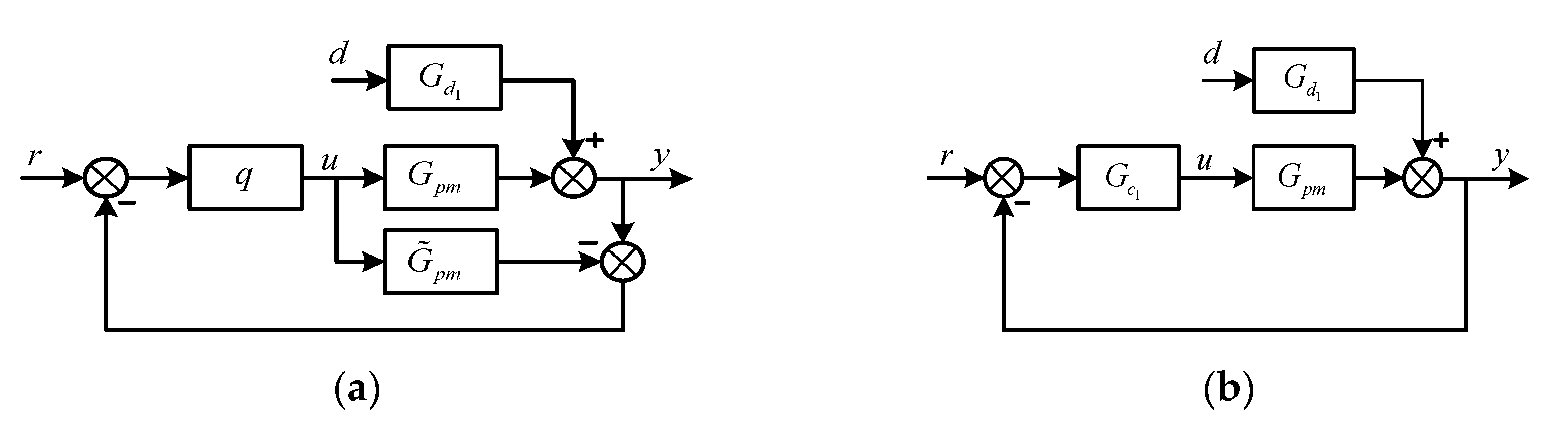
Step 2: Analytical design of the FOPI controller
The ideal feedback controller that is equivalent to the IMC controller can be expressed in terms of the internal model and the IMC controller . Due to the Smith predictor structure, the delay term will be removed in the closed-loop transfer function of the primary loop as in Equation (25). Therefore, in this step, the FOPI controller will be designed for the delay-free process .
Figure 5a,b shows the block diagrams of the IMC scheme and equivalent classical feedback control structures, respectively, where
is the process,
the process model,
the IMC controller, and
the equivalent feedback controller. For the nominal case (
), in
Figure 5a, the system response can be calculated by the set-point and disturbance signals in the following simplified equation:
where
, which is the portion of the model inverted by the controller, and in this case,
(IMC approach is already mentioned in the previous section).
To obtain a good response for processes with poles near zero, the IMC controller should be designed to satisfy the following conditions.
1. If the process has poles near zero at then should have zeros at
2. If the process has poles near zero, then should have zeros at
Since the IMC controller
is designed as
, the first condition is satisfied automatically. The second condition can be fulfilled by designing the IMC filter
as:
where
is an adjustable parameter which controls the tradeoff between the performance and robustness;
is an extra degree of freedom to cancel the poles near zero in
, and determined via the following equation:
Thus, the value of
is obtained as:
Then, the IMC controller is expressed as follows:
From
Figure 5a,b, the ideal feedback controller can be derived in terms of the internal model
and the IMC controller
:
Substituting Equation (46) into Equation (47), the ideal feedback controller is finally obtained:
It is obvious that the resulting controller, Equation (48), does not have the FOPI-type controller form as in Equation (11) and also not in the frequency domain. Therefore, it is necessary to convert it into the frequency domain by replacing
and rearranging it into the complex form. After several calculations, the final result is as follows:
By comparing Equation (49) and Equation (11), the analytical tuning rules of the FOPI controller can be obtained as follows:
From these above equations, two tuning algorithms, Algorithms 1 and 2, for the primary controllers are proposed for case 2, and 3. It is obvious that the control parameters of case 1 are easily obtained.
| Algorithm 1: The proposed tuning algorithm for case 2. |
| 1: Initialization |
Calculate according to Equations (32) and (41)
; ; assign the value of |
| do |
| according to Equation (31) |
| based on Equation (40) |
| according to Equations (50) and (51) |
| for each set of control parameters |
| by: |
| : assign % avoid an infinite loop |
| 9: end while |
| 10: end |
| Algorithm 2: The proposed tuning algorithm for case 3. |
| 1: Initialization |
Calculate according to Equations (36) and (37)
Choose from this range |
| according to Equation (35) |
| 3: Approximate into FOPDT using PSO algorithm |
| based on Equation (40) |
| according to Equations (50) and (51) |
| 6: end |


