Prediction Model of Tunnel Boring Machine Disc Cutter Replacement Using Kernel Support Vector Machine

Abstract

During tunneling processes, disc cutters of a tunnel boring machine (TBM) usually need to be frequently and unexpectedly replaced. Regular inspections are needed to check disc cutters’ status, which significantly reduces the work efficiency and increases the cost. This paper proposes a new prediction model based on TBM operational parameters and geological conditions that determines whether disc cutter replacement is needed. Firstly, an evaluation criterion for whether the cutters need to be replaced is constructed. Secondly, specific parameters related to the evaluation criterion are analyzed and 18 features are established on tunneling monitoring information. Then, the mapping model between the cutter replacement judgement and the established features is built based on a kernel support vector machine (KSVM). Finally, the data obtained from a Jilin water transport tunnel project is utilized to verify the performance of the proposed model. Test results show that the new model can obtain an average accuracy of 90.0% and an average F₁ score of 86.2% on field data prediction based on data from past tunneling days. Therefore, the proposed data-predictive model can be used in tunneling to accurately predict whether disc cutters need to be replaced before human judgment, and thereby greatly improve tunneling safety and efficiency.

1. Introduction

Tunnel boring machines (TBMs) have been widely used in hard rock tunneling due to their high tunneling safety, efficiency, and cost-effectiveness [1,2]. During tunneling, cutterhead rotates with TBM spindle and rocks in front of the TBM are shredded into pieces by disc cutters mounted on the cutterhead. Under poor working conditions, disc cutters often lose efficacy, resulting in the decline of TBM tunneling performance [3]. If the low-efficacy disc cutters are not replaced in time, the possibilities of cutter failures around the disabled disc cutters will increase [4], which may further cause damage to seals, bearings, and even the whole cutterhead, badly affecting the TBM service life. To avoid this kind of situation, frequent inspections and replacements of disc cutters are required during tunneling [5], seriously affecting the construction efficiency. Therefore, considering tunneling safety and efficiency, it is important to detect the status of disc cutters without manual inspections.

Generally, there are mainly six kinds of disc cutter failure patterns, namely normal wear, eccentric wear, flat wear, fracture, local spalling, and secondary wear [6,7,8]. The failures of disc cutters are related to many factors, including rock properties [9], cutter structures [10], materials the disc cutters are made of [11], disc cutter installation positions and arrangements [12], TBM operating parameters [5,8,12], etc. Therefore, prediction of disc cutter failures is a complex multi-input problem.

At present, there are three main methods proposed for obtaining cutter failure information, namely an inspection method, a sensor monitoring method, and a data-driven method.

Regular inspection is the simplest and most reliable method, and thus it is the most widely used method in engineering projects. However, the inspection method is difficult to reflect cutter failures in time, which makes TBM unable to work with the best performance before inspections. Moreover, TBM shutdowns are required for cutter inspections to be carried out, generally at certain times of day or every few strokes. Usually, such downtime of TBMs consumes more than 15% of the tunneling time, greatly reducing the efficiency of the construction and increasing the cost.

Unlike the manual inspection method, the sensor monitoring method allows real-time disc cutter status information to be obtained. However, since sensors are installed on the cutterhead, they are required to work in a harsh working environment of high temperature (70–90 °C), high humidity (80–90% Relative Humidity), and strong vibration (10–20 times the acceleration of gravity), thus resulting in bad performance with detection techniques based on light [13], lubricant addition [14], the magnetoresistive effect [15], or the eddy-current effect [16,17]. Another disadvantage of the sensor monitoring method is that power supply, as well as communication and maintenance of the sensors, are difficult to implement. Therefore, with the sensor-based method, real-time cutter status observation is almost impossible to achieve during tunneling because of sensors’ low reliability. Furthermore, the method is costly because sensors are expensive. For instance, Herrenknecht, a German TBM manufacturer, devised a disc cutter ring wear monitoring device that costs over USD 100,000, not including maintenance costs of damaged disc cutter wear sensors.

Due to the disadvantages of both manual inspection and sensor monitoring methods, data-driven models have become more popular. The data-driven method can predict disc cutter consumption and make maintenance plans before tunneling starts. Generally, the data-driven method can be classified into three kinds—empirical methods [18,19], mechanism-based methods [5,9,20,21,22,23,24,25,26], and tunneling-parameters-based methods [8,12,27,28].

Empirical methods study the regression of cutter health indices and geological parameters based on historical data. Mechanism-based methods use energy theory or mechanical analysis to model the rock breaking process, then the disc cutter wear is mapped with relevant parameters, such as cutterhead rotation speed [20], penetration rate [5], normal force of single disc cutter [23], uniaxial compressive strength (UCS) [9], Cerchar abrasivity index (CAI) [24], cutterhead topological structure [25], and so on. With the disc cutter wear, disc cutter failure can be easily predicted. One major disadvantage of both empirical and mechanism-based methods is that they rely highly on relatively stable geological parameters. However, the geology of tunnels is not immutable; these types of models are thus prone to generating significant errors in real-time prediction.

Fortunately, tunneling-parameters-based prediction methods have proved that working data can reflect the interaction between TBM disc cutters and rocks forward. Benefiting from the current advancement of intelligentization of tunneling [29], TBM operational data can be collected and used in making predictions more effortlessly during tunneling. Acaroglu [27] established a fuzzy logical model to predict specific energy demand in the process of rock cutting with constant cross-section disc cutters based on a linear cutting test result database. Qiao [28] established a genetic programming-based wear life prediction model for shield disc cutters, using tree-shaped expression to reflect the relationship between cutter wear and relevant parameters (namely, rotating speed, excavation distance, penetration depth, disc cutter spacing width, and disc cutter installation radius). To estimate the life of the earth-pressure-balance shield machine, Khalid [8] proposed a genetic algorithm (GA) optimized group method of data handling (GMDH)-type neural network (NN) that used shield operational parameters (namely, thrust force, penetration rate, and cutter rotation speed) and geological conditions (i.e., uniaxial compressive strength) as model inputs. Meanwhile, after proposing a new disc cutter health index defined as the ratio of the rolling distance of disc cutters to their maximum rolling distance, Yu [12] established a map between the new health index and 412 data features based on a one-dimensional convolutional neural network. These models focus on predicting the wear of each disc cutter. However, there is no need to monitor the status of each cutter during tunneling. For tool detection of a milling machine, the overall cutting performance is more concerned than the specific value of wear on each blade [30,31,32]. Likely, determining whether the cutting ability of the cutterhead has decreased is necessary to predict whether a disc cutter replacement is needed during tunneling, which is consistent with the human judgment standard.

Therefore, the question of predicting disc cutter replacements is fundamentally a binary classification problem of a cutterhead’s cutting performance. Considering the computational cost applied to projects, in this paper, a Gaussian kernel support vector machine prediction model is built for predicting disc cutter replacements using operational data and prior geological information. After being trained on a period of historical data, the proposed model can accurately predict in a real-time manner whether disc cutter replacement is needed, which reduces the time consumed by regular inspections. The main highlights of the proposed method are that it only takes the easily collected data as model input and complex cutter monitoring sensors are not needed; hence it can easily be deployed during construction. In addition, prior geological survey data are used to build the model, thereby it can acquire good performance in different tunneling projects. The rest of this paper is arranged as follows. Section 2 introduces a disc cutter replacement evaluation function and presents the proposed SVM method. Section 3 gives a review of the studied project and how the data was collected. Then, a modelling process and result analysis of the proposed method are demonstrated in Section 4. Finally, Section 5 provides our conclusion.

2. The Proposed Prediction Framework

2.1. Evaluation Function and Related Parameters

As mentioned in the introduction section, the major reason to replace low-efficacy disc cutters is because cutting with them is not efficient under manual judgement. Therefore, a disc cutter evaluation criterion is needed to estimate the ability of disc cutters during tunneling. The most common and intuitive health index is abrasion loss of cutter rings, which is difficult to measure. Several other health indices have been proposed to indirectly estimate the ability. Bruland [21,33] took the excavated tunnel length per disc cutter as the health index of disc cutter performance. Hassanpour [9] proved that disc cutter life, which is defined as the length of time a disc cutter has been working before replacement, is more suitable to estimate disc cutter life. Yu [12] took into account the different rolling distances of disc cutters at different positions based on excavated tunnel length, and calculated the rolling distance of each disc cutter as the health index based on an equidistant cylindrical spiral. All these studies focused on indirect measurements of abrasion loss. However, changes of disc cutter ability result in changes of TBM rock-breaking ability. In this paper, a qualitative evaluation criterion for cutting ability is proposed to estimate disc cutters’ ability.

The studied TBM is an open-type girder TBM, widely used in tunneling with good surrounding rock integrity. The main components of an open-type girder TBM are shown in Figure 1. The tunneling procedures of an open-type girder TBM can generally be summarized as follows:

Step 1: Tunneling preparation. At this stage, the gripper (10) is pressed on the excavated tunnel wall by stretching out the gripper cylinders. Then the back support (11) is withdrawn and the cutterhead drive motors (5) are started to get the cutterhead (1) ready for tunneling.

Step 2: Rock breaking and advancing. The thrust cylinders (9) located on either side of the girder are stretched out. The cutterhead (1) is pushed against the rock before it and rotates with the spindle (3) driven by the motors (5). The rock surface is crushed by disc cutters (2) mounted on the cutterhead to form concentric circular grooves. With the increase in the depth of the grooves, the cracks on the surface become deepened and intersected. Then rocks between adjacent concentric circular grooves flake off to form rock fragments. At the same time, the rock fragments are collected by the scraper on the cutterhead. Then they slide through the cutterhead (1) to the inside of the TBM, and are finally carried out of the tunnel through the belt conveyor (8). If soft or broken strata are encountered during the excavation, it is often necessary to stop the extension of the thrust cylinders (9) and shut down the cutterhead.

Step 3: Regripping and position adjusting. At this stage, the back support (11) extends and the gripper (10) retracts. The thrust cylinders (9) also retract, thus pulling the gripper ahead.

The TBM is constantly switching and circulating between these three steps until the tunneling is completed. In tunnel construction, the process of the above three steps is called a “stroke” of TBM,

Disc cutters work in Step 2 above. Therefore, the field parameters in Step 2 are needed to estimate disc cutter conditions. A feasible calculation of disc cutters’ cutting ability evaluation under different geological conditions referring to the specific energy [20,26] is as follows:

$$ca={\mathrm{f}}_1\left(rock properties\right)w_{1}F+{\mathrm{f}}_2\left(rock properties\right)w_2\frac{T}{p}$$

(1)

where ca is cutting ability evaluation, ${\mathrm{f}}_1$ and ${\mathrm{f}}_2$ are functions of rock properties, $w_1$ and $w_2$ are weight coefficients, $F$ is thrust, $T$ is cutterhead torque, and $p$ is penetration rate. The cutting ability evaluation can be simplified as:

$$ca={\alpha }_{1}F+{\alpha }_2\frac{T}{p}$$

(2)

where α₁ and ${\alpha }_2$ are variable coefficients about geological conditions.

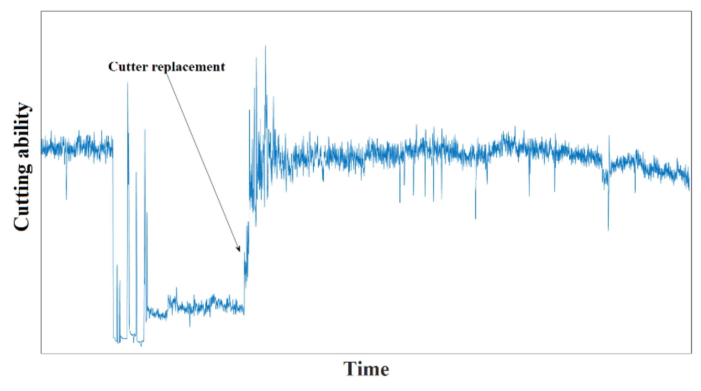
For a short piece of continuous rock formation where rock properties usually do not change much, ${\alpha }_1$ and ${\alpha }_2$ can be approximately treated as invariant. The cutting ability evaluation before and after a cutter replacement in one day was calculated and is shown in Figure 2. To observe the changing trend of cutting ability evaluation, only the data of rock breaking and advancing procedure is shown. The ability of the cutters can be observed from the changing trend of the curve in the figure. For example, cutting ability evaluation begins to change drastically and eventually stabilizes at a lower value before disc cutter replacement. On the contrary, cutting ability evaluation gets a big boost after disc cutter replacement, and as the time goes on, it generally decreases until the next disc cutter replacement is performed. The oscillation in the figure occurs because the mechanical model of TBM rock breaking is periodically changing every second even under uniform geology. Furthermore, there are outliers that do not follow the trend mainly because the geological conditions have changed in these parts.

If Equation (1) is used for quantitative judgement of the cutting ability, there are two main problems: (1) the specific rock properties are difficult to obtain during tunneling; (2) the functions associated with rock properties, ${\mathrm{f}}_1$ and ${\mathrm{f}}_2$, are complex nonlinear. However, previous research has proved that TBM operational parameters can be used to predict rock information because they reflect the rock–machine interactions [34]. Therefore, it is possible to approximate real-time geological conditions with prior geological information and operational parameters, such as advance rate, thrust, cutterhead torque, cutterhead rotational speed, advance mileage, penetration rate, etc. Thus, Equation (1) can be transformed as an expression of known data:

$$\begin{array}{c}ca={\mathrm{f}}_1\left(\mathrm{f}\left(prior geological information, operational parameters\right)\right)w_{1}F\\ +{\mathrm{f}}_2\left(\mathrm{f}\left(prior geological information, operational parameters\right)\right)w_2\frac{T}{p}\end{array}$$

(3)

From Equation (3), one may see that the cutting ability evaluation is affected by both geological features and operational parameters. Therefore, Equation (3) is highly complex and nonlinear. However, a threshold is enough to determine whether the disc cutters should be replaced for making cutter maintenance plans. As shown in Figure 2, the cutting ability evaluation when disc cutter replacement is needed and when TBM works normally are highly different. The question then becomes a classification problem of the results of Equation (3). Considering the complexity of the model deployment in projects, this paper provides a cost-sensitive Gaussian kernel support vector machine for predicting whether disc cutters need to be replaced. The performance of the proposed model and some other common algorithms are shown in Section 4.

2.2. Introduction of Support Vector Machine

A support vector machine (SVM) is a supervised machine learning technique used to separate classes [30,31,32,35,36]. SVM is widely used in tunneling research, such as ultimate strength prediction [37], geological prediction [38], and TBM performance prediction [39].

Similar to the logistic regression method, SVM is based on the linear function ${\omega }^{T}x+b$, but the output of SVM is a classification judgement, rather than a probability. If ${\omega }^{T}x+b$ is positive, SVM prediction belongs to the positive class; If ${\omega }^{T}x+b$ is negative, SVM prediction belongs to the negative class.

Because SVM is a linear classification model and the cutter replacement evaluation criterion is nonlinear with respect to tunneling data, classification using SVM directly will obtain poor results. The most important reason for the current wide application of SVM is the use of the kernel technique. The basis of the kernel technique is that many machine learning algorithms can be written as dot products between samples. For example, a linear function in SVM can be rewritten as:

$${\omega }^{T}x+b=b+{\displaystyle \sum }_{i=1}^m{\alpha }_i{x}^T{x}^{\left(i\right)}$$

(4)

where, $x^{\left(i\right)}$ is a training sample of TBM operational data and prior geological information, and $\alpha$ is coefficient vector.

After replacing x with the output of eigenfunction $\varnothing \left(x\right)$ and replacing the dot product by the kernel function $k(x,x^{\left(i\right)})=\varnothing \left(x\right)·\varnothing \left(x^{\left(i\right)}\right)$, we can use the following function to make the cutter replacement prediction $f\left(x\right)$:

$$f\left(x\right)=b+{\displaystyle \sum }_i{\alpha }_{i}k\left(x^T{x}^{\left(i\right)}\right)$$

(5)

This function is non-linear about x, but it is linear about $\varnothing \left(x\right)$. The relationship between $\alpha$ and $f\left(x\right)$ is also linear. $f\left(x\right)$ preprocesses all the inputs with $\varnothing \left(x\right)$, and then learns the linear model in the new transformation space.

The kernel technique enables SVM to learn nonlinear models (functions of x) using convex optimization techniques that ensure effective convergence. Because $\varnothing$ is fixed, only $\alpha$ needs optimizing, which means that the optimization algorithm can treat the decision functions as linear functions in different spaces and build hyperplanes to separate the data sets. In our paper, a Bayesian optimization algorithm is used to optimize hyper-parameters.

In most cases, even though $\varnothing \left(x\right)$ is hard to calculate, $k(x,x^{\prime })$ is easy to calculate. The Gaussian kernel, also known as the radial basis function (RBF), is provided by:

$$k\left(x,x^{\prime }\right)=exp\left(-\frac{1}{2}{\left(x-x^{\prime }\right)}^T{{\displaystyle \sum }}^{}{\left(x-x^{\prime }\right)}^{-1}\right)$$

(6)

where ∑ is the covariance of each feature in the observations, a p-dimensional matrix.

Because ∑ is ball-shaped, the kernel function of TBM operational data and prior geological information is:

$$k\left(x,x^{\prime }\right)=exp\left(-\frac{{\Vert x-x^{\prime }\Vert }^2}{2{\sigma }^2}\right),{\sigma }_j=\sigma ,\forall j$$

(7)

where ${\sigma }_j$ is the characteristic length scale of the jth feature.

Assuming that the value of the category label is 0 or 1, which represents negative samples (need replacement) and positive samples (normal operation), the optimal classification hyperplane established by a sample $y_i$ for SVM conforms to the following formula:

$$y_i\left(W^{T}X+b\right)>0, i=1,2,\dots ,n$$

(8)

where

$$\tilde{\gamma }=y_i\left(W^{T}X+b\right) ,i=1,2,\dots ,n$$

(9)

is called function distance.

To solve the coefficients, the objective function of SVM optimization is:

$$\max \left(\gamma =\frac{\left|W^{T}X+b\right|}{\Vert \omega \Vert }\right)$$

(10)

When $\tilde{\gamma }=1$, the distance between the support vector and the optimal classification hyperplane is $\frac{1}{\Vert \omega \Vert }$ and the distance between two support vectors is $\frac{2}{\Vert \omega \Vert }$. Hence, the objective function is transformed to:

$$\max \left(\frac{2}{\Vert \omega \Vert }\right)$$

(11)

which equals

$$\min \left(\frac{{\Vert \omega \Vert }^2}{2}\right)$$

(12)

Equation (12) is fundamentally the original question of constrained optimization. By constructing a Lagrange function, one gets:

$$L\left(\alpha ,\omega ,b\right)=\frac{{\Vert \omega \Vert }^2}{2}-{\displaystyle \sum }_{i=1}^n\alpha ·\left[y_i(W^T{x}^i+b\right)-1]$$

(13)

When $\frac{\partial L}{\partial \omega }=0$,

$$\omega ={\displaystyle \sum }_{i=1}^n{\alpha }_i\ast x_i\ast y_i$$

(14)

and when $\frac{\partial L}{\partial b}=0$,

$${\displaystyle \sum }_{i=1}^n{\alpha }_i\ast y_i=0$$

(15)

Substituting Equations (14) and (15) into the Lagrange function $L\left(\alpha ,\omega ,b\right)$, one may get:

$$L\left(\alpha ,\omega ,b\right)={\displaystyle \sum }_{i=1}^n{\alpha }_i-\frac{{{\displaystyle \sum }}_{i=1}^n{\alpha }_i{\alpha }_j{y}_i{y}_j{x}^T{x}_j}{2}$$

(16)

After solving for an optimal solution $\alpha$, the corresponding $\omega$and $b$ can be calculated.

However, the optimal classification hyperplane solved cannot always perfectly categorize whether a cutter replacement is needed. In order to solve the misclassification problem, a relaxation factor $\xi$ is introduced. In this situation, the optimal classification hyperplane established by a sample $y_i$ for SVM conforms to the following formula:

$$y_i\left(W^{T}X+b\right)\ge 1-{\xi }_i ,i=1,2,\dots ,n$$

(17)

When 0 < $\xi$ < 1, the sample point $y_i$ can be correctly classified into two categories, namely needing replacement and operating normally. However, if $\xi \ge 1$, there will be misclassifications. The penalty term $c{{\displaystyle \sum }}_{i=1}^n{\xi }_i$ is introduced to avoid misclassifications. In this case, the objective function Equation (12) is transformed to:

$$\varphi \left(\omega ,\xi \right)=\frac{{\Vert \omega \Vert }^2}{2}+c{\displaystyle \sum }_{i=1}^n{\xi }_i$$

(18)

where $c$ is a constant penalty factor. By adjusting the classification cost matrix in Equation (18), the SVM model becomes cost-sensitive and can focus on failure samples.

3. Data Sources Description

3.1. Project Summary

In this paper, the fourth section of the Jilin water transport tunnel with a total excavation diameter of 8033 mm is taken as our research object. Geologically, the section is mainly composed of tuff, conglomerate, carboniferous limestone, albite porphyry, quartz diorite, and granite, as shown in Figure 3.

This tunnel was excavated using an open-type TBM. The project started on 7 July 2015 and ended on 4 February 2018. The effective tunneling days of the TBM were 728 days, after deducting the drilling-blasting time, maintenance time, and bad geological downtime. Among those 728 days, cutters replacements occurred in a total of 312 days.

3.2. Introduction to Studied TBM

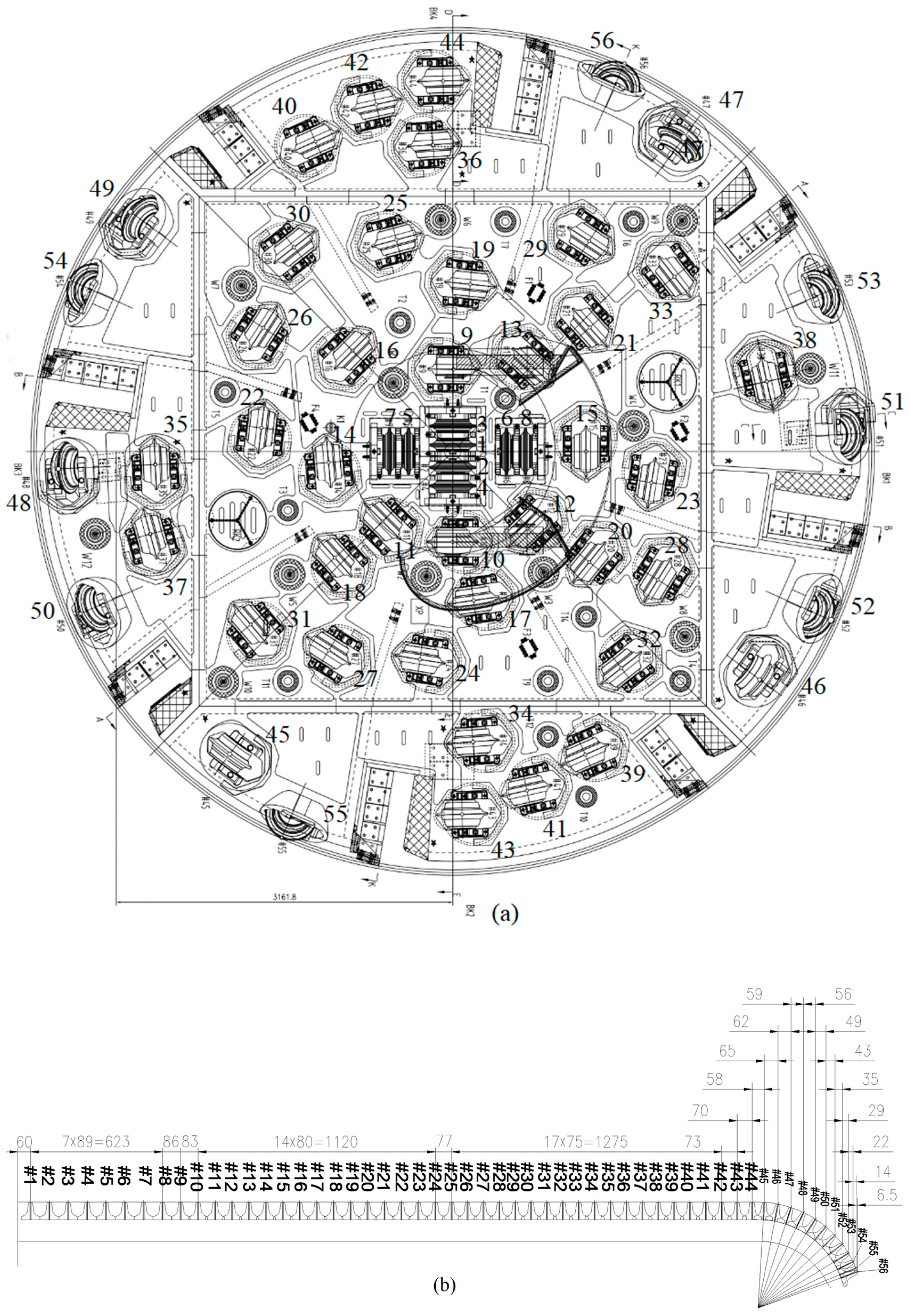
The main technical parameters of the whole TBM and its cutterhead are shown in

Table 1. Technical parameters of the studied TBM.

Models	Technical Parameter	Parameter Value
Whole TBM	Main part length	20 m
	Main part quality	615 t
	Regripping time	5 min
	Trusting stroke	1800 mm
Cutterhead	Diameter	7930 mm
	Number of central disc cutters	6
	Central disc cutter diameter	432 mm
	Number of face disc cutters	38
	Face disc cutter diameter	483 mm
	Number of gage disc cutter	12
	Gage disc cutter diameter	483 mm
	Space between disc cutters	82 mm/80 mm

. Figure 4a shows the positions of all 56 disc cutters on the cutterhead, including 6 central disc cutters, 38 face disc cutters and 12 gage disc cutters. Figure 4b shows that disc cutters with larger serial numbers have farther distances from the center of the cutterhead. In addition, the number of disc cutters in the same circle increases as the circumference increases.

3.3. TBM Data and Geological Survey Data

During tunneling, field data of the TBM were collected every second. The TBM operational data had 199 kinds of monitoring data. They were collected from subsystems of the TBM, including cutterhead system, driving system, supporting system, belt conveyor system, electrical system, and hydraulic system.

As for the geological parameters, a preliminary check of geological conditions was carried out through boreholes before excavating. During tunneling, the geological changes were carefully monitored by geological engineers via observation of the conditions of fragments cut by the TBM. Once the degree of rock fragmentation was considered to be changed, the rock samples were tested to determine different parameters such as rock-saturation uniaxial compressive strength and fissure coefficient, and then rock mass basic quality was calculated according to [40]. Although the results of geological surveys did not reveal the whole geological conditions of the tunnel, application of image processing technology made it possible to monitor geological changes through rock fragments in real time [41].

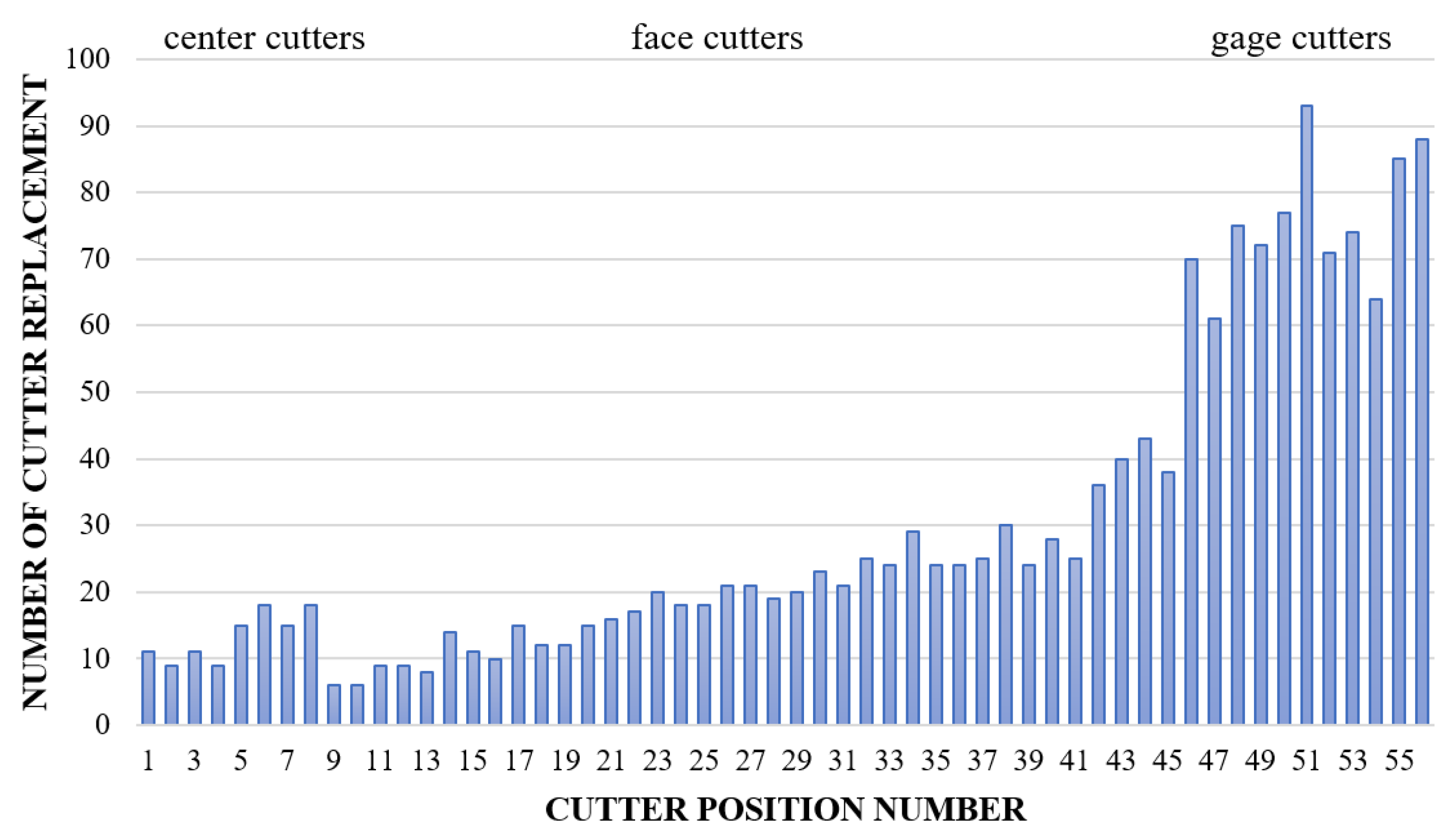
Besides daily inspections, disc cutter conditions were inspected routinely after three strokes of TBM excavating. During inspections, disc cutters over their wear limit and abnormal disc wear cutters were replaced. In this study case, 1692 disc cutters were replaced. The total numbers of disc cutter replacements in each position are shown in Figure 5. As can be seen from Figure 5, the central disc cutters were less often replaced because they had a small radius compared to their diameter. The low numbers of central and face disc cutter replacements were mainly related to their position radii. For gage disc cutters there was no obvious pattern.

4. Validation and Analysis

To verify the feasibility and effectiveness of the proposed method, TBM operational data, geological survey data, and field cutter replacement data from Jilin water transport tunnel were used to build datasets. Then, the datasets were used to train and validate the proposed model. In this section, the performance indices of the model are shown and compared with the results of other models.

4.1. Data Preparation

It is important to point out that cutting ability evaluation cannot be directly calculated based on the monitoring data from the Jilin water transport tunnel according to Equation (3). However, to validate the classification performance of the proposed model, the datasets were divided into two groups. Only short pieces of data before disc cutter replacements were classified as “replacement needed” data. The data of working days on which no disc cutter replacements occurred were randomly selected as “no replacement needed” data. More specifically, the “replacement needed” data were constructed from the data before replacements in a total of 278 cases, and the “no replacement needed” data were constructed from the data of a total of 416 no-disc-cutter-replacement days. The detailed data preprocessing procedures are shown below.

4.1.1. Extraction of TBM Thrusting Phases

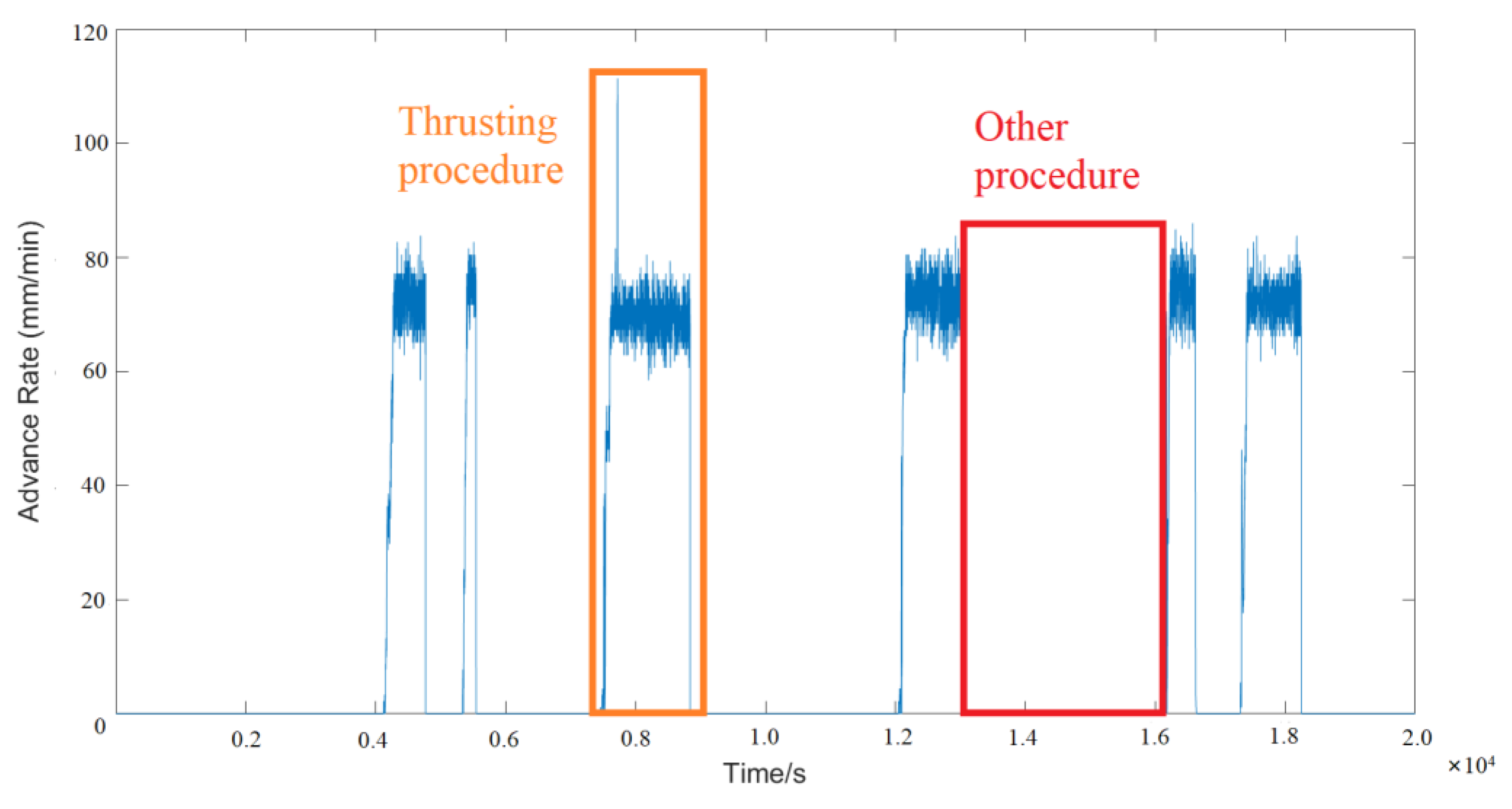
As mentioned above, the TBM working process comprises three procedures: gripping, thrusting, and regripping. Additionally, there are downtimes for regular inspections and maintenance during tunneling. Hence, a large amount of irrelevant data, as the other procedure data shown in Figure 6, should be extracted from the original TBM operational data.

The TBM raw operational data comprises multiple TBM operational parameters. The data apart from the thrusting procedure can be removed from the TBM raw operational database according to [34]:

$$\mathrm{P}=\mathrm{f}\left(RSP\right)\mathrm{f}\left(T\right)\mathrm{f}\left(F\right)\mathrm{f}\left(V\right)$$

(19)

where $RSP$ is cutterhead rotational speed, $T$ is cutterhead torque, $F$ is thrust, and $V$ is advance rate. If one of them is equal to zero, then p = 0, which means that the TBM is not in the thrusting procedure.

The zeros recognition function f(x) is defined as

$$\mathrm{f}\left(x\right)=\{\begin{array}{c}0 x=0\\ 1 x\ne 0\end{array}$$

(20)

4.1.2. Parameter Selection

Equation (3) shows that cutting ability evaluation is related to the operational and geological parameters. Among the operational parameters, there is a certain relationship between some parameters. Merging parameters with high correlation can help remove redundant parameters and reduce the computational cost of data mining. The simplest way to determine whether these parameters are interrelated is to calculate the Pearson correlation coefficient ρ among the operational parameters, as shown in Equation (21):

$$\rho \left(X,Y\right)=\frac{COV\left(X,Y\right)}{{\sigma }_X{\sigma }_Y}$$

(21)

where $\rho \left(X,Y\right)$ is the Pearson correlation coefficient between variable X and Y, $COV\left(X,Y\right)$ is the covariance of variable X and Y, while ${\sigma }_X$ and ${\sigma }_Y$ are the standard deviations of X and Y, respectively.

The major TBM cutterhead and driven system parameters monitored and recorded include advance rate ($V$), thrust ($F$), cutterhead torque ($T$), cutterhead rotational speed ($RSP$), advance mileage (AM), advance displacement (AD), penetration rate ($p$), drive motor current (I), drive motor torque (MT), and drive motor frequency (MF). These 10 parameters were randomly sampled from the trusting data extracted in Section 4.1.1 and used for correlation analysis. The correlation analysis results of 160,000 sets of data are shown in

Table 2. Correlation analysis results of randomly sampled data.

$\mathit{\rho }$	V	F	T	RSP	AM	AD	$\mathit{p}$	I	MT	MF
V	1
F	0.06	1
T	0.11	0.76	1
RSP	0.05	0.51	0.34	1
AM	−0.03	0.35	0	−0.02	1
AD	0.06	0.21	0.34	0.09	−0.03	1
$p$	0.99	0.04	0.1	0	−0.03	0.06	1
I	0.1	0.78	0.95	0.46	0.06	0.31	0.08	1
MT	0.11	0.76	1	0.34	0	0.34	0.1	0.95	1
MF	0.05	0.5	0.33	1	−0.02	0.09	0	0.45	0.33	1

.

Generally, when $\left|\rho \right|\ge 0.8$, the two parameters are considered to be strongly correlated. As shown in Table 2, the following parameters are strongly correlated: advance rate ($V$) and penetration rate ($p$); drive motor current (I), torque (MT), and cutterhead torque ($T$); cutterhead rotational speed ($RSP$) and drive motor frequency (MF). Therefore, some of them can be removed to reduce the model’s complexity. Eventually, the following eight parameters were chosen as input variables:

(1)

(Rock type: Unlike subway tunnel construction, hard rock tunnel construction may encounter more flexible geological conditions. Generally, different types of rock have different value ranges of petrophysical parameters.

(2)

Uniaxial compressive strength: The measurement of the strength characteristics of rock materials, which is widely used to represent geological conditions in previous research.

(3)

Advance rate: The derivative of advance displacement, which is related to the TBM forward velocity.

(4)

Trust: The pressure of the thrust cylinders, which provides the major power of driving TBM forward.

(5)

Cutterhead rotational speed: The angular velocity of cutterhead rotating with TBM spindle, which is related to the relative velocity of cutter to rock.

(6)

Advance mileage: The displacement distance of TBM during the whole tunneling, which is related to the rolling distances of disc cutters.

(7)

Advance displacement: When TBM works in the gripping-thrusting-regripping procedure, the propulsion cylinders reach out and retract cyclically. Advance displacement is the stroke of propulsion cylinders.

(8)

Drive motor current: The electric current of the drive motor operating at constant power mode, which shows the working power of the drive motors.

4.1.3. Denoising and Normalization

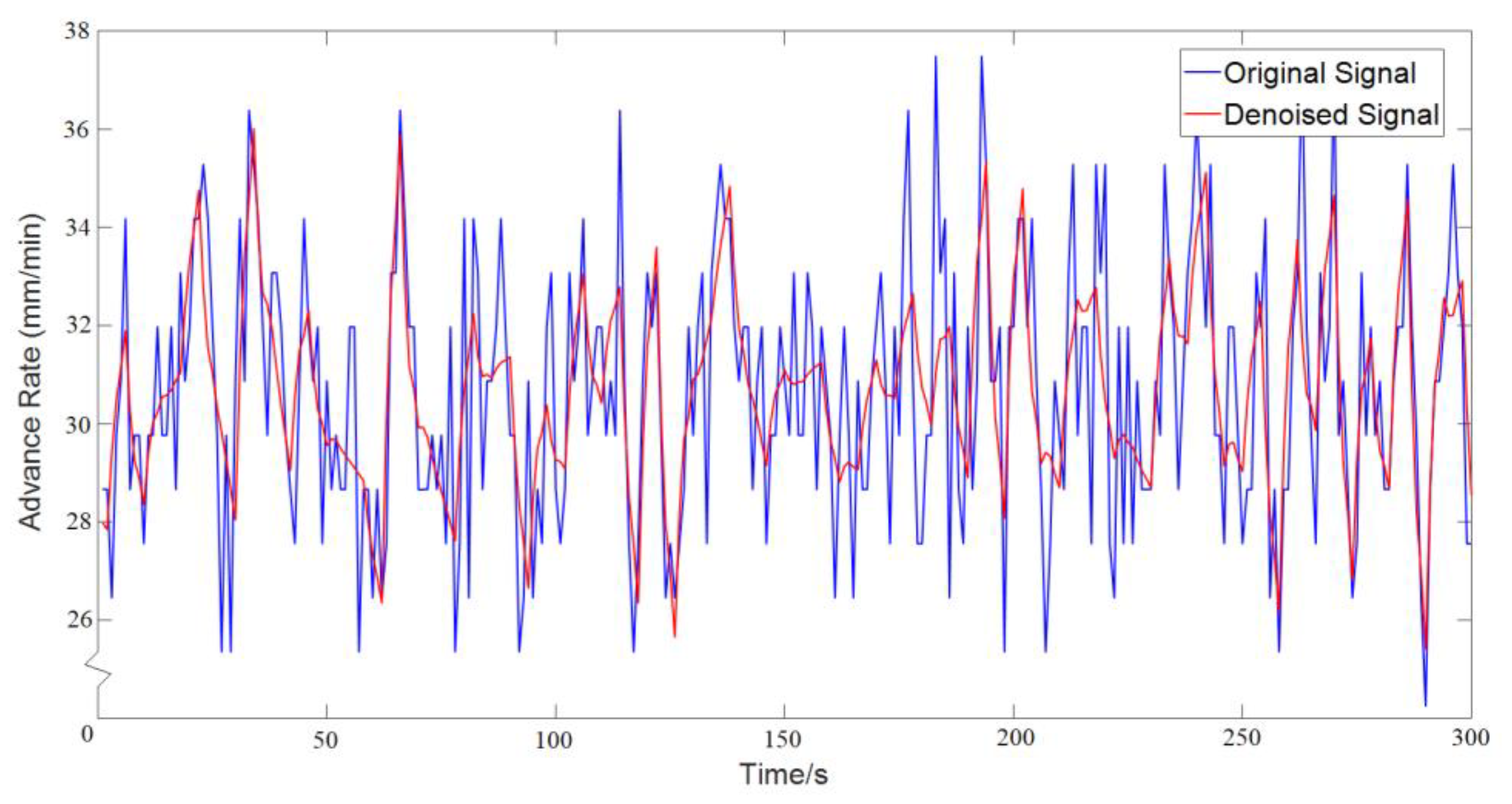
In order to improve the data quality, the raw TBM trusting data are denoised by a wavelet filter. More specifically, the DB3 wavelet is selected to decompose the original data into two layers, and then the data are reconstructed by using soft threshold segmentation. The original TBM operational data and denoised data with wavelet filter are shown in Figure 7.

Due to the outliers in the original signal, the traditional min-max normalization method performs poorly. To calculate the normal value range of the data, Tukey’s boxplot data ranges [42,43,44] was used in this paper.

In this study, the TBM operational data objects are curves. Let $\mathsf{{\rm B}}=\{\beta :D\to R^d|\beta$ is absolutely continuous} be the space of absolutely continuous parametrized curves from d-dimensional Euclidean space. Define $SO\left(d\right)=\{R\in R^{d\times d}|R^{T}R=R{R}^T=I_d,\det \left(R\right)=\mp 1\}$ as the rotation group, and $\mathsf{\Gamma }=\{\gamma :D\to D|\gamma$ is an orientation-preserving diffeomorphism} as the reparameterization group.

For a curve $\beta \in \mathsf{{\rm B}}$, its square-root velocity function (SRVF) $q:D\to R^d$ is defined using a mapping $Q:\mathsf{{\rm B}}\to L^2\left(D,R^d\right)$ as

$$q=Q\left(\beta \right)=\frac{\dot{\beta }}{\sqrt{\dot{\beta }}}$$

(22)

where $|·|$ is the Euclidean norm in $R^d$ and $\dot{\beta }$ is the time derivative of $\beta$.

Shape distance is defined in [44] as

$$D_s\left(\left[q_1\right],\left[q_2\right]\right)=\underset{\gamma \in \mathsf{\Gamma },R\in SO\left(d\right)}{\min }co{s}^{-1}(\langle q_1,R\left(q_2,\gamma \right)\rangle )$$

(23)

where $\left[q\right]=\left\{R\left(q,\gamma \right)|\left(\gamma ,R\right)\in \mathsf{\Gamma }\times SO\left(d\right)\right\}$ is the orbit of q, $·,·$ is the $L^2$ inner product. Then the median of a sample of SRVFs $\left\{q_1,\cdots ,q_n\right\}$ is

$$\left[\overline{q}\right]=arg\underset{\left[q\right]\in C/\left(\mathsf{\Gamma }\times SO\left(d\right)\right)}{\min }{\displaystyle \sum }_{i=1}^n{D}_s\left(\left[q\right],\left[q_i\right]\right)$$

(24)

The data are ordered according to their distances from the median, then two shape quartiles $\left({\mathsf{\upsilon }}_{Q_1},{\mathsf{\upsilon }}_{Q_3}\right)$ are acquired based on 50% central data. Given the two quartiles, the shape interquartile range (IQR) is defined as the sum of the shape distances from each quartile to the median:

Then, the maximum and minimum of the normal value range are defined as:

$$IQ{R}_s=\Vert v_{Q_1}\Vert +\Vert v_{Q_3}\Vert$$

(25)

$$\mathsf{\upsilon }{w}_1={\mathsf{\upsilon }}_{Q_1}+k_s\times IQ{R}_s\times \frac{v_{Q_1}}{\Vert v_{Q_1}\Vert }$$

(26)

$$\mathsf{\upsilon }{w}_3={\mathsf{\upsilon }}_{Q_3}+k_s\times IQ{R}_s\times \frac{v_{Q_3}}{\Vert v_{Q_3}\Vert }$$

(27)

The choice of $k_s$ represents the tolerance for outliers. In this paper, the normal value range can include mild outliers, thus $k_s=3$ is selected. Then, the eight parameters chosen as input variables are scaled according to their value range to avoid situations where partial features dominate the model.

4.1.4. Time Feature Construction

Since tunneling is a dynamic process, data of a certain time are difficult to precisely reflect precise disc cutter conditions. Therefore, features are extracted from time series data. The time window of the data object for feature extraction is selected as 5 min. The average value, peak value, variance, and other augmented features are calculated to represent the 5 min data. Specific chosen features about the eight parameters are shown in

Table 3. Selected parameters and their augmented features.

Parameters	Features Value
Rock type	Type index
UCS	Average value
Advance rate	Average value, Peak value, Variance
Trust	Average value, Peak value, Variance
RSP	Average value, Peak value, Variance
Advance mileage	Interval value from the last disc cutter replacement
Advance displacement	Sample range
Drive motor current	Maximum, Minimum, Average value, Peak of 10 motor current variance, Peak of 5 min motor current kurtosis index

.

Most of the time, cutterhead cutting ability is above the judgement threshold and no disc cutter replacement is required during tunneling. The size of “no replacement needed” data is larger than that of “replacement needed” data. Therefore, different sampling ratios are required to equalize the data sets. For “no replacement needed” data, 5 min samples are randomly sampled from the data of 414 no-disc-cutter replacement days. For “replacement needed” data, a sliding time window is used to acquire more 5 min samples from the time before disc cutter replacements, whose rolling distance is set to 5 s.

Eventually, a total of 46,629 instances from 691 days were used to construct the training and testing sets. Among them, 16,852 instances were “replacement needed” data and 29,777 instances were “no replacement needed” data. Each instance had 18 features and a class label. The numerical output value of normal operation was set to 1 and that of predicted failure was set to 0. To evaluate the model performance during training, a 10-fold cross-validation was used to obtain the errors.

To reproduce our process, the original data of the studied project can be found at https://github.com/ChenZuyuIWHR/YS-IWHR, accessed on 16 February 2022.

4.2. Study Results and Discussion

To evaluate the performance of a classifier, the confusion matrix for binary classification problems is showed in

Table 4. Confusion matrix for binary classification problems.

	Predicted Class	Positive	Negative
True Class
Positive		TP (true positive)	FN (false negative)
Negative		FP (false positive)	TN (true negative)

.

Precision rate of a binary classifier is given by:

$$\mathrm{Precision}=\frac{N_{TP}}{N_{TP}+N_{FP}}$$

(28)

Recall rate of a binary classifier is:

$$\mathrm{Recall}=\frac{N_{TP}}{N_{TP}+N_{FN}}$$

(29)

The classification model for classifier evaluation is based on precision rate and recall rate. As shown in Equations (28) and (29), when $N_{FP}$ and $N_{FN}$ change, precision rate and recall rate change inversely, hence the optimization goal for most models is to improve one of the rates while guaranteeing the other. $F_{\beta }$ score is used when these two targets come into conflict. $F_{\beta }$ combines the precision and recall rates into a single score, where the weight of recall rate is $\beta$ times that of precision rate. The most common $F_1$ score takes recall rate to be as important as accuracy rate:

$$F_1=2·\frac{\mathrm{precision}·\mathrm{recall}}{\mathrm{precision}+\mathrm{recall}}$$

(30)

The 46,629 instances were divided into training set and testing set according to a 4:1 ratio. The five most commonly used classification algorithms were compared with KSVM, namely decision tree (DT), k-nearest neighbors (KNN), naive Bayesian (NB), convolutional neural network (CNN), and stacked autoencoder (SAE). The Bayesian optimization was used to find the best hyper-parameters of the former four machine learning models. For KSVM, optimized hyper-parameters are kernel function, kernel scale, box constraint level, and penalty factor; For DT, optimized hyper-parameters are maximum number of splits and split criteria; For k-NN, optimized hyper-parameters are the number of neighbors, distance metric, and distance weight; For NB, optimized hyper-parameters are distribution and kernel type. For deep learning algorithms, several layers are used in CNN and SAE to extract deep features from input parameters. The specific hyper-parameters and their corresponding performance results are shown in

Table 5. Hyper-parameters and performance results of 6 classification models.

Models	Best Hyper-Parameters	Test Performance				Training Time/s
		Accuracy	Precision	Recall	F1
KSVM	Kernel function: Gaussian Kernel scale: 1.05 Box constraint level: 500 Penalty factor: 3	98.1%	98.7%	98.3%	98.5%	1316
DT	Number of splits: 693 Split criteria: Minimized deviations	95.6%	97.1%	95.9%	96.5%	432
KNN	Number of neighbors: 3 Distance metric: Hamming Distance weight: Inverse Distance Weighting	96.8%	99.2%	95.8%	97.5%	866
NB	Distribution: Kernel Kernel type: Gaussian	72.8%	78.3%	79.9%	79.1%	2151
CNN	Number of convolutional layer: 6 Dropout rate: 0.3	98.9%	99.9%	98.3%	99.1%	6500
SAE	Number of stacked autoencoder: 4	99.0%	99.4%	98.9%	99.2%	5219

. Because KSVM showed a good prediction performance among six models and can acquire this accuracy with a short training time, it was thus selected as a tool to predict disc cutter replacements.

In some publications [12,45], it is believed that TBM operational data is enough to reflect accurate information of the tunnel geological conditions, thus geological data are not considered as an input. In

Table 6. Average performance results of the proposed model with and without geological inputs.

Models	Test Performance
	Accuracy	Precision	Recall	F1
Operational data KSVM	94.4%	97.0%	94.1%	95.6%
Operational and geological data KSVM	98.1%	98.7%	98.3%	98.5%

, a model with only operational data as inputs is compared with the proposed KSVM model, which uses both operational and geological data. More specifically, the former uses 16 features as inputs, ignoring two geological features. As Table 6 shows, although geological survey information can not accurately reflect the geological conditions of every moment, it can reveal the approximate range of geological conditions, thus significantly improving the prediction performance.

During tunneling, it is often expected that the data collected from the finished part can be used to guide the construction of the unfinished part. Over a continuous period of time, as collected data increase, the interaction between TBM disc cutters and rocks becomes clearer and a more accurate prediction model can be built. To validate this assumption, the trainings of the proposed model on different lengths of time spanning a month, half a month, and a week were conducted, and their corresponding predictions of disc cutter replacements for the following two days were compared. The comparison results are given in

Table 7. Prediction results after different training time lengths.

Training Time Length	Test Performance
	Accuracy	Precision	Recall	F1
One month	72.7%	59.1%	83.0%	71.1%
Half a month	90.0%	98.7%	73.6%	86.2%
One week	82.2%	78.7%	80.4%	79.6%

.

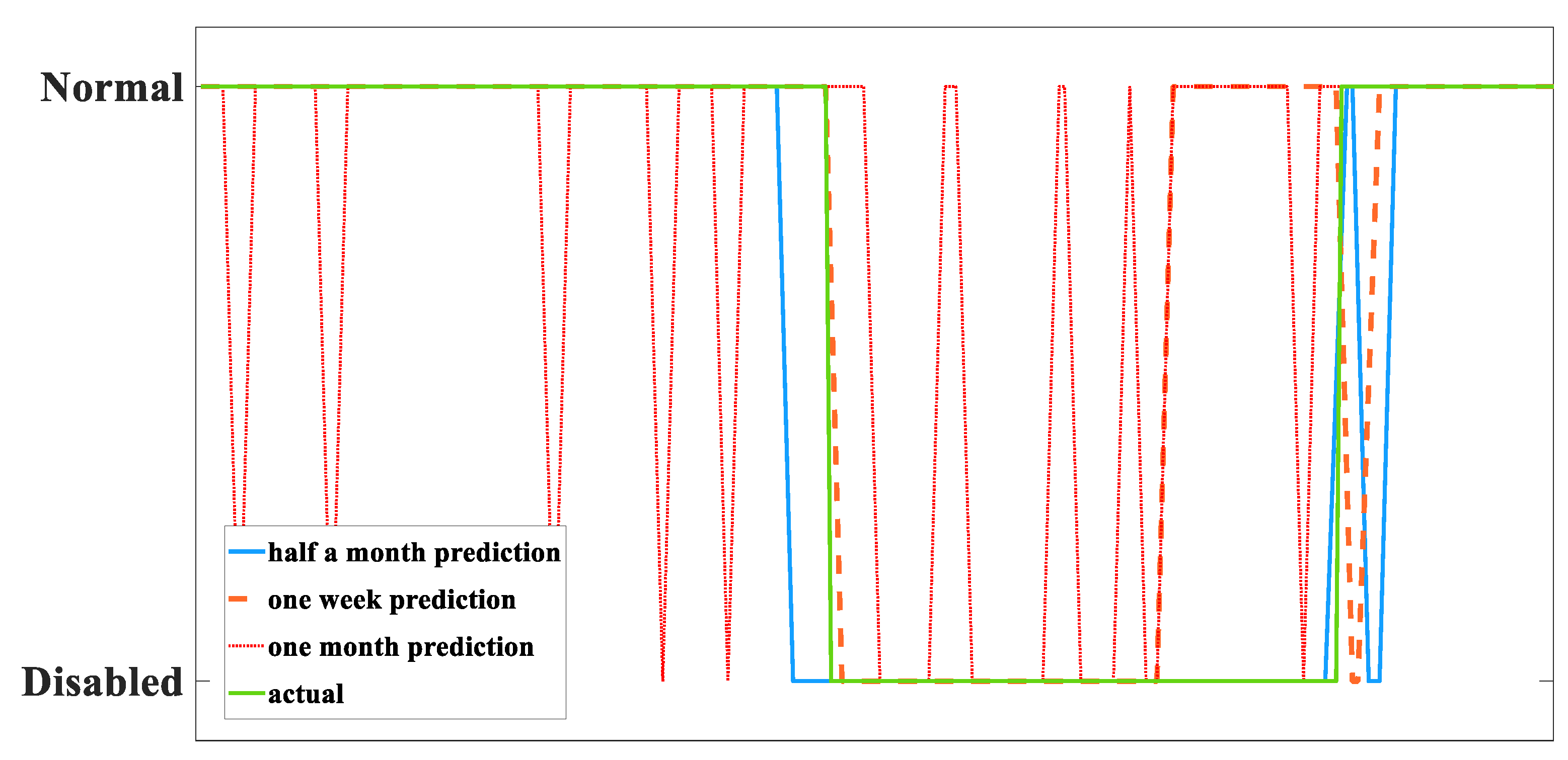
As Table 7 shows, the best result is not as good as the result after training on the whole dataset. This is mainly because some rock-cutter interactive modes are not included in the training set of a short period of time. However, from the hypothesis in Section 2.1, for a short piece of time, the rock properties usually do not change much. Therefore, Table 7 shows that data of a short time, about 15 days, can generate an accuracy of 90.0%. When the training time length decreased from one month to half a month, the average prediction precision rate increased from 59.1% to 98.7%. Although recall rate decreased from 83.0% to 73.6%, the increase in precision was more helpful in tunneling because false positives are far more unacceptable than false negatives. The prediction performance turned down when the training time length decreased from half one month to a week, due to the small sample size of one-week training data sets. In some extreme cases, no disc cutter replacements are carried out within a whole week; therefore, the proposed method cannot learn “replacement needed” conditions in such situations. In Figure 8, the receiver operating characteristic (ROC) curve of these classification models is presented. It can be seen that the area under the curve (AUC) of the proposed KSVM model based on the data of 15 continuous days is the highest. In Figure 9, the predicted values of these classification models are presented. The proposed KSVM model based on one-month data performed poorly. Its predicted value oscillated throughout the whole process. For disc cutters from normal to “replacement needed”, the prediction of one-week model was fast and accurate. However, as the orange line in Figure 9 shows, the one-week model was prone to predicting wrongly when disc cutters needed replacement. As for the KSVM model based on the data of 15 continuous days, the predicted value changed before cutter failure and remained correct when the cutters needed replacement. As for new data after cutter replacement, the half-month model could perceive well the change of cutters’ performance. These results show that the proposed KSVM model can generate an average accuracy of 90.0% and an average $F_1$ score of 86.2%, performing well in terms of high accuracy, robustness, and stability.

Generally, disc cutter wear processes are entirely different among different tunnel projects. To prove the adaptability of our method, the proposed KSVM model was tested on an earth pressure balance (EPB) shield machine dataset in Guangdong.

The geological conditions are different between the Jilin and Guangdong projects [46]. Geologically, the tunnel section in Guangdong is mainly composed of backfill, silty clay, weathered rock, and weathered granite. According to [40], the rock formation of Guangdong tunnel is mainly soft rock, while that of Jilin tunnel is mainly hard rock. The mean value of rock UCS in Guangdong is 32, compared with 163 in Jilin. In addition, the tunneling equipment used in the two projects was quite different. The boring machine in Guangdong had six more central cutters and its face cutters were aligned rather than misaligned. During tunneling, compared with the Jilin project, the Guangdong boring machine had a greater trusting force, a slower cutterhead rotational speed, and a higher penetration rate. The proposed model can provide 88.8% accuracy and 93.1% $F_1$ score prediction performance, compared with 90.0% accuracy and 86.2% $F_1$ score on the Jilin project. The results show that the proposed model can be deployed in different projects even if the working conditions are highly different.

5. Conclusions

This paper presents a method to predict whether TBM disc cutters need replacement based on both operational and geological data. Through the study of historical disc cutter replacement data, this method can automatically predict whether a cutter replacement is needed after a current stroke, without installation of more sensors. This method also decreases the time consumed with regular manual inspections. Firstly, several methods were adopted to eliminate irrelevant data and improve the data quality effectively. Then, eight parameters were chosen from the processed tunneling data and 18 features were extracted to reflect time series information. Lastly, after comparing six different prediction algorithms, the proposed cost-sensitive Gaussian kernel support vector machine with an average accuracy of 98.1% and an average $F_1$ score of 98.5% was selected as the prediction model.

The test results on a Jilin’s water transport tunnel dataset show that a 15-day training of the proposed model can provide 90.0% accuracy and 86.2% $F_1$ score prediction performance on untrained data of the following two days. Moreover, the proposed model was tested on data from another project in Guangdong and acquired 88.8% accuracy and a 93.1% $F_1$ score. The results show that the proposed cutter replacement prediction procedure could be applied in different tunneling projects, which can help with making disc cutter replacement plans. Therefore, our proposed method can reduce overall cutter inspection time and sensor cost usually required for disc cutter replacement. In addition, fewer manual inspections and on-time disc cutter replacements also mean higher tunneling safety.

To further develop this study, it is very important to find a method to monitor geological changes online; more accurate rock properties information can thus be collected to train the proposed model. In addition, although 18 features were selected to build a reliable cutter replacements prediction model, other parameters could be tested for enhancing the overall prediction model’s performance. For example, cutterhead structure data, such as cutter diameter, distances between cutters, and position radii may be used to generate higher prediction accuracy.

References

1. Liu, Q.; Huang, X.; Gong, Q.; Du, L.; Pan, Y.-C.; Liu, J.-P. Application and development of hard rock TBM and its prospect in China. Tunn. Undergr. Space Technol. 2016, 57, 33–46. [Google Scholar] [CrossRef]
2. Zheng, Y.; Zhang, Q.; Zhao, J. Challenges and opportunities of using tunnel boring machines in mining. Tunn. Undergr. Space Technol. 2016, 57, 287–299. [Google Scholar] [CrossRef]
3. Hassanpour, J.; Rostami, J.; Azali, S.T.; Zhao, J. Introduction of an empirical TBM cutter wear prediction model for pyroclastic and mafic igneous rocks; a case history of Karaj water conveyance tunnel, Iran. Tunn. Undergr. Space Technol. 2014, 43, 222–231. [Google Scholar] [CrossRef]
4. Liu, Q.; Liu, J.-P.; Pan, Y.-C.; Zhang, X.; Peng, X.; Gong, Q.; Du, L. A Wear Rule and Cutter Life Prediction Model of a 20-in. TBM Cutter for Granite: A Case Study of a Water Conveyance Tunnel in China. Rock Mech. Rock Eng. 2017, 50, 1303–1320. [Google Scholar] [CrossRef]
5. Wang, L.; Li, H.; Zhao, X.; Zhang, Q. Development of a prediction model for the wear evolution of disc cutters on rock TBM cutterhead. Tunn. Undergr. Space Technol. 2017, 67, 147–157. [Google Scholar] [CrossRef]
6. Yang, J.-H.; Zhang, X.-P.; Ji, P.-Q.; Liu, Q.-S.; Lu, X.-J.; Wei, J.-P.; Qi, S.-H.; Fang, H.-G.; Fang, J.-N.; Geng, Y.-J. Analysis of disc cutter damage and consumption of TBM1 section on water conveyance tunnel at Lanzhou water source construction engineering. Tunn. Undergr. Space Technol. 2018, 85, 67–75. [Google Scholar] [CrossRef]
7. Elbaz, K.; Shen, S.-L.; Cheng, W.-C.; Arulrajah, A. Cutter-disc consumption during earth pressure balance tunnelling in mixed strata. Proc. Inst. Civ. Eng.-Geotech. Eng. 2018, 171, 363–376. [Google Scholar] [CrossRef]
8. Elbaz, K.; Shen, S.-L.; Zhou, A.; Yin, Z.-Y.; Lyu, H.-M. Prediction of Disc Cutter Life During Shield Tunneling with AI via the Incorporation of a Genetic Algorithm into a GMDH-Type Neural Network. Engineering 2020, 7, 238–251. [Google Scholar] [CrossRef]
9. Hassanpour, J. Development of an empirical model to estimate disc cutter wear for sedimentary and low to medium grade metamorphic rocks. Tunn. Undergr. Space Technol. 2018, 75, 90–99. [Google Scholar] [CrossRef]
10. Schneider, E.U.P.D.-I.E.; Thuro, U.P.D.R.N.K.; Galler, U.P.D.-I.D.R. Forecasting penetration and wear for TBM drives in hard rock—Results from the ABROCK research project/Prognose von Penetration und Verschleiß für TBM-Vortriebe im Festgestein—Erkenntnisse aus dem Forschungsprojekt ABROCK. Géoméch. Tunn. 2012, 5, 537–546. [Google Scholar] [CrossRef] [Green Version]
11. Zhang, X.; Lin, L.; Xia, Y.; Tan, Q.; Zhu, Z.; Mao, Q.; Zhou, M. Experimental study on wear of TBM disc cutter rings with different kinds of hardness. Tunn. Undergr. Space Technol. 2018, 82, 346–357. [Google Scholar] [CrossRef]
12. Yu, H.; Tao, J.; Huang, S.; Qin, C.; Xiao, D.; Liu, C. A field parameters-based method for real-time wear estimation of disc cutter on TBM cutterhead. Autom. Constr. 2021, 124, 103603. [Google Scholar] [CrossRef]
13. Zhao, H.L.; Sun, Z.C.; Chen, K.; Wang, H.Z.; Yang, Y.D.; Zhou, J.J.; Li, F.Y.; Zhang, B.; Song, F.L. Synthesis, Property and Wear Detection of Disc Cutter for Shield Tunneling Machine of Nanobelt Ca0.68Si9Al3(ON)16: Eu2+ Luminescence Fibers. J. Inorg. Mater. 2018, 33, 866–872. [Google Scholar] [CrossRef]
14. Gharahbagh, E.A.; Mooney, M.A.; Frank, G.; Walter, B.; DiPonio, M.A. Periodic inspection of gauge cutter wear on EPB TBMs using cone penetration testing. Tunn. Undergr. Space Technol. 2013, 38, 279–286. [Google Scholar] [CrossRef]
15. Gong, Q.; Wu, F.; Wang, D.; Qiu, H.; Yin, L. Development and Application of Cutterhead Working Status Monitoring System for Shield TBM Tunnelling. Rock Mech. Rock Eng. 2021, 54, 1731–1753. [Google Scholar] [CrossRef]
16. Wang, F.; Men, C.; Kong, X.; Meng, L. Optimum Design and Application Research of Eddy Current Sensor for Measurement of TBM Disc Cutter Wear. Sensors 2019, 19, 4230. [Google Scholar] [CrossRef] [Green Version]
17. Lan, H.; Xia, Y.; Ji, Z.; Fu, J.; Miao, B. Online monitoring device of disc cutter wear—Design and field test. Tunn. Undergr. Space Technol. 2019, 89, 284–294. [Google Scholar] [CrossRef]
18. Karami, M.; Zare, S.; Rostami, J. Tracking of disc cutter wear in TBM tunneling: A case study of Kerman water conveyance tunnel. Bull. Eng. Geol. Environ. 2020, 80, 201–219. [Google Scholar] [CrossRef]
19. Hassanpour, J.; Rostami, J.; Zhao, J.; Azali, S.T. TBM performance and disc cutter wear prediction based on ten years experience of TBM tunnelling in Iran. Géoméch. Tunn. 2015, 8, 239–247. [Google Scholar] [CrossRef]
20. Sun, Z.; Yang, Y.; Chen, K.; Li, F.; Zhou, J.; Zhang, B.; Chen, Q. Disc Cutter’s Rock Breaking Ability and Wear Resistance in Extremely Hard Rock: A Case Study in Qinling Tunnel of Han River to Wei River Water Diversion Project. Geotech. Geol. Eng. 2019, 37, 4901–4910. [Google Scholar] [CrossRef]
21. Zare, S.; Bruland, A. Applications of NTNU/SINTEF Drillability Indices in Hard Rock Tunneling. Rock Mech. Rock Eng. 2012, 46, 179–187. [Google Scholar] [CrossRef]
22. Gehring, K. Performance and cutter-wear prediction for tunnel boring machines. Felsbau 1995, 13, 439–448. [Google Scholar]
23. Wang, L.; Kang, Y.; Zhao, X.; Zhang, Q. Disc cutter wear prediction for a hard rock TBM cutterhead based on energy analysis. Tunn. Undergr. Space Technol. 2015, 50, 324–333. [Google Scholar] [CrossRef]
24. Ko, T.Y.; Lee, S.S.; Ko, T.Y. Effect of Rock Abrasiveness on Wear of Shield Tunnelling in Bukit Timah Granite. Appl. Sci. 2020, 10, 3231. [Google Scholar] [CrossRef]
25. Park, B.; Lee, C.; Choi, S.-W.; Kang, T.-H.; Chang, S.-H. Discrete-Element Analysis of the Excavation Performance of an EPB Shield TBM under Different Operating Conditions. Appl. Sci. 2021, 11, 5119. [Google Scholar] [CrossRef]
26. Zhao, Y.; Yang, H.; Chen, Z.; Chen, X.; Huang, L.; Liu, S. Effects of Jointed Rock Mass and Mixed Ground Conditions on the Cutting Efficiency and Cutter Wear of Tunnel Boring Machine. Rock Mech. Rock Eng. 2018, 52, 1303–1313. [Google Scholar] [CrossRef]
27. Acaroglu, O.; Ozdemir, L.; Asbury, B. A fuzzy logic model to predict specific energy requirement for TBM performance prediction. Tunn. Undergr. Space Technol. 2008, 23, 600–608. [Google Scholar] [CrossRef]
28. Qiao, J.L.; Meng, Q.J.; Liu, J.Q.; Jin, J.X. Prediction of wear life of shield disc cutter in complex formations based on genetic pro-gramming. Ind. Mine Autom. 2018, 9, 51–58. [Google Scholar] [CrossRef]
29. Yang, H.Y. Progress and Trend of Construction Machinery Intelligence. Constr. Mach. Technol. Manag. 2017, 12, 19–21. [Google Scholar] [CrossRef]
30. Zhang, C.; Zhang, H. Modelling and prediction of tool wear using LS-SVM in milling operation. Int. J. Comput. Integr. Manuf. 2015, 1–16. [Google Scholar] [CrossRef]
31. Sun, S.; Hu, X.; Cai, W.; Zhong, J. Tool Breakage Detection of Milling Cutter Insert Based on SVM. IFAC-PapersOnLine 2019, 52, 1549–1554. [Google Scholar] [CrossRef]
32. Kong, D.; Chen, Y.; Li, N.; Duan, C.; Lu, L.; Chen, D. Tool Wear Estimation in End Milling of Titanium Alloy Using NPE and a Novel WOA-SVM Model. IEEE Trans. Instrum. Meas. 2019, 69, 5219–5232. [Google Scholar] [CrossRef]
33. Bruland, A. Hard Rock Tunnel Boring. Trondheim. Ph.D. Thesis, Norwegian University of Science and Technology, Trondheim, Norway, 2000. [Google Scholar]
34. Zhang, Q.; Liu, Z.; Tan, J. Prediction of geological conditions for a tunnel boring machine using big operational data. Autom. Constr. 2019, 100, 73–83. [Google Scholar] [CrossRef]
35. Fan, J.; Lee, J.; Lee, Y. A Transfer Learning Architecture Based on a Support Vector Machine for Histopathology Image Classification. Appl. Sci. 2021, 11, 6380. [Google Scholar] [CrossRef]
36. Li, X.; Yang, Y.; Pan, H.; Cheng, J.; Cheng, J. A novel deep stacking least squares support vector machine for rolling bearing fault diagnosis. Comput. Ind. 2019, 110, 36–47. [Google Scholar] [CrossRef]
37. Di, Q.; Wu, Z.; Chen, T.; Chen, F.; Wang, W.; Qin, G.; Chen, W. Artificial intelligence method for predicting the maximum stress of an off-center casing under non-uniform ground stress with support vector machine. Sci. China Technol. Sci. 2020, 63, 2553–2561. [Google Scholar] [CrossRef]
38. Tinoco, J.; Correia, A.G.; Cortez, P. Support vector machines applied to uniaxial compressive strength prediction of jet grouting columns. Comput. Geotech. 2014, 55, 132–140. [Google Scholar] [CrossRef]
39. Xu, H.; Zhou, J.; Asteris, P.G.; Armaghani, D.J.; Tahir, M.M. Supervised Machine Learning Techniques to the Prediction of Tunnel Boring Machine Penetration Rate. Appl. Sci. 2019, 9, 3715. [Google Scholar] [CrossRef] [Green Version]
40. CJWRC. Standard for Engineering Classification of Rock Mass. GB/T 50218-2014. 2014. Available online: https://ebook.chinabuilding.com.cn/zbooklib/bookpdf/probation?SiteID=1&bookID=59005 (accessed on 16 February 2022).
41. Yang, Z.; He, B.; Liu, Y.; Wang, D.; Zhu, G. Classification of rock fragments produced by tunnel boring machine using convolutional neural networks. Autom. Constr. 2021, 125, 103612. [Google Scholar] [CrossRef]
42. Sun, Y.; Genton, M.G. Functional Boxplots. J. Comput. Graph. Stat. 2011, 20, 316–334. [Google Scholar] [CrossRef]
43. Mirzargar, M.; Whitaker, R.T.; Kirby, R.M. Curve Boxplot: Generalization of Boxplot for Ensembles of Curves. IEEE Trans. Vis. Comput. Graph. 2014, 20, 2654–2663. [Google Scholar] [CrossRef]
44. Xie, W.; Chkrebtii, O.; Kurtek, S. Visualization and Outlier Detection for Multivariate Elastic Curve Data. IEEE Trans. Vis. Comput. Graph. 2019, 26, 3353–3364. [Google Scholar] [CrossRef] [PubMed]
45. La, Y.S.; In, K.M.; Bumjoo, K. Prediction of replacement period of shield TBM disc cutter using SVM. J. Korean Tunn. Undergr. Space Assoc. 2019, 21, 641–656. [Google Scholar] [CrossRef]
46. Elbaz, K.; Shen, S.-L.; Zhou, A.; Yin, Z.-Y.; Lyu, H.-M. Data in intelligent approach for estimation of disc cutter life using hybrid metaheuristic algorithm. Data Brief 2020, 33, 106479. [Google Scholar] [CrossRef] [PubMed]
Figure 1. Diagram of main structure of an open-type girder TBM (1. Cutterhead; 2. Disc cutter; 3. Spindle; 4. Top shield; 5. Cutterhead drive motor; 6. Steel arch assembly machine; 7. Jumbolter; 8. Belt conveyor; 9. Thrust cylinder; 10. Gripper; 11. Back support).
Applsci 12 02267 g001
Figure 2. Cutting ability evaluation of the studied TBM before and after disc cutter replacements during 13 August 2015.
Applsci 12 02267 g002
Figure 3. Geological section map of Jilin water transport tunnel (part).
Applsci 12 02267 g003
Figure 4. (a) Structure of the TBM cutterhead; (b) Schematic diagram of the cutterhead.
Applsci 12 02267 g004
Figure 5. Number of disc cutter replacements at each position.
Applsci 12 02267 g005
Figure 6. TBM advance rate during operation.
Applsci 12 02267 g006
Figure 7. Original and denoised TBM advance rate.
Applsci 12 02267 g007
Figure 8. ROC curve of classification models on test sets.
Applsci 12 02267 g008
Figure 9. Comparison of predicted and actual conditions of TBM disc cutters from 6 to 12 June 2016.
Applsci 12 02267 g009