Performance Prediction and Optimization of Multi-Mirror Combined Solar Dish Collector

Abstract

An analytical method to calculate and optimize the performance of a multi-mirror combined solar dish collector is proposed in this work. It is based on the method of directly calculating the optical efficiency of a reflecting point, which can consider the influence of many factors. The distribution of the reflected solar intensity is obtained by the convolution of the actual solar intensity distribution and Gaussian distribution of the optical error. Then, the optical efficiency for a single mirror is calculated through integration over the total area of the mirror, and the method is validated by the SolTrace code. It is a rather quick method that reduces the amount of calculation and keeps high accuracy. The heat loss per unit area for the cavity receiver is assumed to be constant at a definite operation temperature for performance analysis and optimization. Taking a 62.25 m² combined dish system with 249 square spherical mirrors as an example, the effects of system focal length, open radius of receiver, optical error, and focal length of the mirror on the system intercept factor and efficiency are studied. An optimization model is developed for maximizing the annual average net thermal efficiency. If the mirrors used have the same focal length for reducing the manufacture cost, when the optical error is 2 mrad, the net thermal efficiency and the intercept factor of the optimized system are 85.87% and 98.60%, respectively, while the concentration ratio is about 2000.

1. Introduction

Concentrated solar thermal systems are among the most cost-effective ways to replace fossil fuel. The parabolic solar dish system is a highly valued concentrated solar thermal system because of its high concentration ratio and efficiency at high temperatures [1]. Both the thermal and the optical efficiency of parabolic dish collectors are the highest among all concentrators [2]. They use parabolic mirrors to concentrate solar rays on the focal point where their energy can be converted and transported by a receiver [3]. The mirror can be one large, smooth mirror or be made of a number of smaller mirrors.

The manufacture of a large-area monolithic parabolic mirror requires a high level of technology and cost. Therefore, a combination of small mirrors is generally used, which means that a number of small mirrors are fixed on the structure to let their center form a large paraboloid.

Using spherical mirrors instead of parabolic mirrors can keep performance and greatly reduce the processing difficulty, and it is a common manufacturing method for a combined dish system. In 1988, Hedgepeth and Miller [4] proposed an outer space solar dish concentrator system in the NASA report, composed of hexagonal and square spherical mirrors. In 1993, an 87.7 m² combined square mirror dish concentrating system was developed with an output power of 90 kW and optical efficiency of about 88% [5]. The Australian National University (ANU) designed and produced a 400 m² combined dish system named ‘SG3′ in 2003 that consists of identical multi-triangle spherical mirror to reduce the cost of production [6]. A similar system was subsequently constructed at the Ben Gurion University in Israel [7]. Later, in 2011, ANU designed and built a 500 m² multi-mirror combined system [2]. It contained 380 identical 1.17 m × 1.17 m spherical mirrors with a focal length of 13.4 m. In the same year, Li [8] proposed a multi-mirror combined technology that uses multiple flat mirrors to form a dish shape. In 2012, Liu [9] designed an 8.15 kW combined dish system consisting of 164 flat mirrors, and analyzed the effects of the mirror size and position on optical performance.

There are three types of method for the optical performance simulation of solar dish concentrators in the literature. The first method is the ray tracing method which is a microscopic method and can be applied in most cases, where it can provide an enormous amount of numerical information. It is easy to code and has been developed by many researchers [10,11,12], but it obscures functional relationships and is time-consuming, as pointed out by Bendt and Rabl [13].

The second method is to first calculate the solar energy flux at the receiver surface, and then the total intercepted energy is obtained through integration; many functions have been proposed to predict the flux at the receiver. The first function for calculating the radiation flux of the solar dish receiver was proposed by Hukuo and Mii [14], which is based on the assumption that the solar radiation source is a uniform disc. Later, some similar distribution equations were proposed by Hiester [15], O’Neill, and Hudson [16] with the same assumption. In fact, it is different from a real solar disc because of the effect of solar limb darkening [17]. Trombe [18] considered the brightness distribution of the solar disc, but ignored the solar halo and the optical error of the concentrator. Biggs and Vittltoe [19] considered the elliptical distribution of the optical error to propose a general function for a solar concentrator which was applied in the Helios program. It was further developed in the CIRCE program [20] for performance analysis of various solar dish concentrating collectors. However, both of these functions for calculation of the radiation flux at the receiver surface are too complicated to integrate analytically; thus, a numerical method is often preferred. On the basis of the Gaussian brightness distribution approximation, Bendt and Rabl [13] presented an angular acceptance function for both flat and sphere receivers to calculate the optical efficiency. Stine and Harrigan [21] reported a different equation which was also based on the Gauss approximation.

The third method is to directly calculate the optical efficiency of a paraboloid dish solar concentrator with a cavity [22] or sphere [23] receiver solar dish system, which is fast while ensuring accuracy. The optical performance of a solar dish system is affected by many factors, such as geometric concentration ratio, rim angle, focal length, and optical error of mirrors [22]. Hafez and Soliman [24] introduced that the optimization of system performance is closely related to the rim angle of the system, receiver size, and concentration ratio. There have been many studies on the performance analysis and optimization of solar parabolic dish concentrators for typical single-mirror systems, but there is little research on combined dish systems except for the solar trace.

In the performance analysis of multi-mirror combined solar dish systems, Johnston et al. [25] applied a ray tracing method to predict the flux density distribution of a 400 m² solar combined dish system. Using this method, the optical performance of 54 triangular spherical mirrors in the system was further analyzed in 2003 [6]. Lovegrove et al. [2] applied the ray tracing method to evaluate the optical performance of a 500 m² square spherical multi-mirror combined dish concentrating system and preliminarily demonstrated that the optimized combined dish system can achieve a geometric concentration ratio of more than 2000. Huang [26] developed a design and optimization analysis of a combined dish system containing 16 mirrors. They calculated the flux density distribution of the receiver under different optical errors and focal plane radii using the Monte Carlo ray tracing method. A similar analysis was also performed for this combined system [27]. Wang et al. [28] conducted a study on a combined dish system consisting of 450 square mirrors of 0.1 m × 0.1 m, and used TracePro software to analyze the flux density distribution of two concentrator surfaces.

Currently, ray tracing is the main method to study the optical performance of a combined dish system. However, this method requires tracking a large number of rays to obtain high accuracy, which is very time-consuming and difficult to use for system optimization; accordingly, only some specific designs have been studied.

In this work, using the previously developed method of directly calculating the optical efficiency of concentrators [29], a new model for the optical efficiency calculation of a combined dish system is first proposed, and the accuracy of this method is validated by the SolTrace code. Then, the optical performance of a combined solar dish system composed of 249 spherical mirrors is studied using the method. The effects of the receiver radius, system focal length, optical error, and mirror focal length on the optical performance of the combined disc system are analyzed. Lastly, in order to maximize the annual average net thermal efficiency, an optimization model is developed, and the optimal design parameters of the combined dish system are calculated.

2. Method: The Optical Efficiency Calculation Model and Optimization Method for Combined Dish System

2.1. Combined Spherical Mirrors Dish System Design

Small-sized square spherical mirrors were installed on the frame structure of the solar dish system. The size of each mirror was 0.5 m × 0.5 m, and the total mirror area of the system was 62.25 m². The system had nine layers in both vertical and horizontal directions, with a total of 249 mirrors. An octagonal solar dish system centered on the bottom mirror is shown in Figure 1.

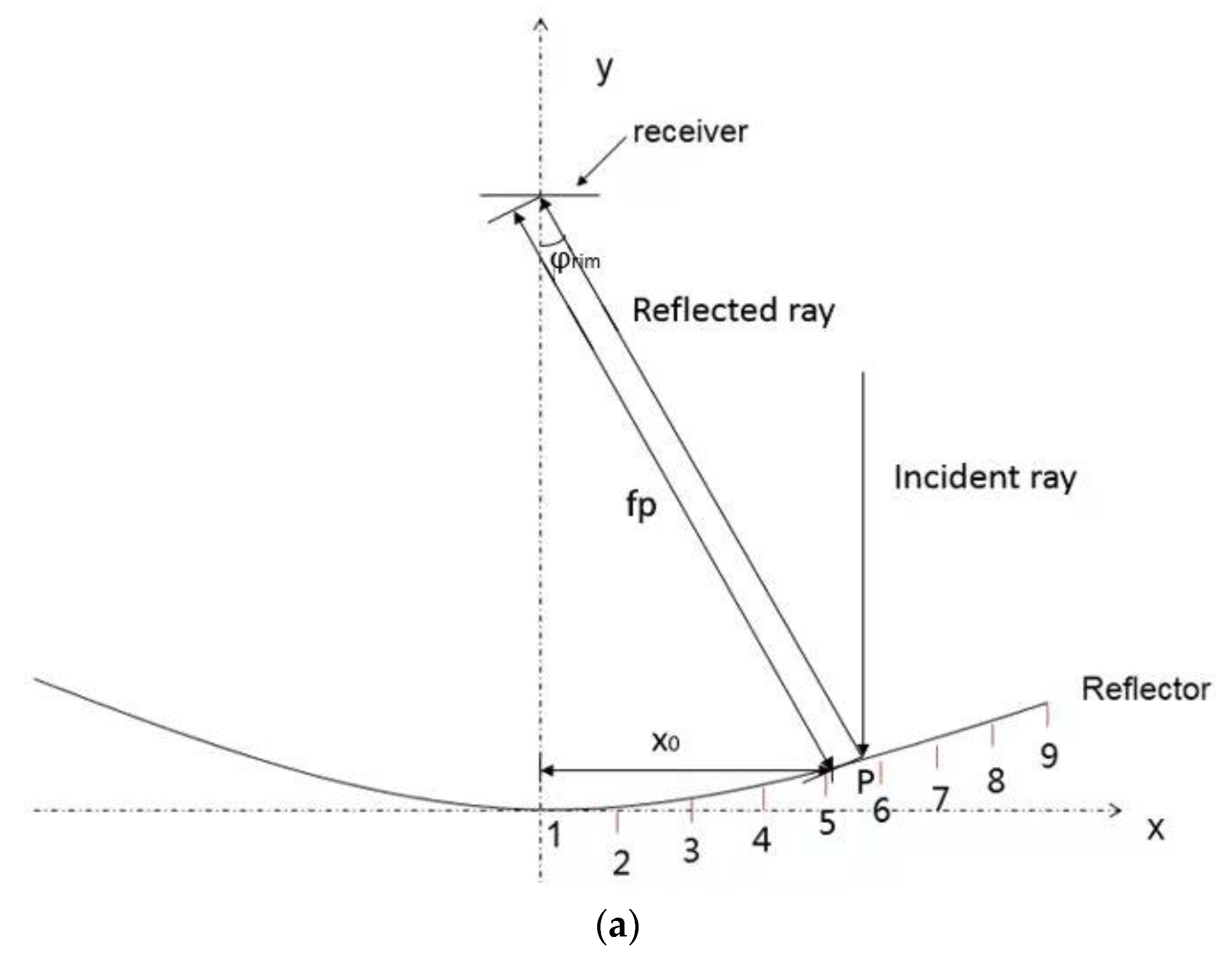
The distance from the reflection point P to the center of the receiver is

$$f_p=\frac{2f_0}{1+\cos \left({\phi }_{rim}\right)},$$

(1)

where f₀ is the system focal length, and φ_rim is the rim angle of the mirror.

$$sin{\phi }_{rim}=\frac{x_0}{f_p},$$

(2)

where x₀ is the vertical distance from the reflection point p to the principal axis.

Therefore, it can be obtained from Equations (1) and (2) that

$${\phi }_{rim}=2\times {\tan }^{-1}\frac{x_0}{2\times f_0}.$$

(3)

2.2. Optical Efficiency Calculation Model for Combined Dish System

We previously proposed a method to calculate the optical efficiency of a rectangular spherical mirror with a rectangular receiver [29]. The model developed in this work converts the square receiver to a circular receiver. The calculation principle is similar, as briefly introduced below.

For a reflection point P of the dish system, the reflected light intensity distribution is B_eff (θ). As shown in Figure 2, the central solar ray from the sun is reflected at point P to intersect with the receiver at point O. The center solar ray OP is set as the z-axis. When the light cone reaches the reference plane U which is perpendicular to the z-axis and passes point O, a circular light spot is formed. If the angle between the light ray and the central solar ray is θ, the radiation energy reflected from point P absorbed by the receiver can be expressed as follows [30]:

$$I_p=f_{at}\ast f_{rec}{\iint }_D{B}_{eff}(\theta )d\phi \sin \theta d\theta ,$$

(4)

where f_at is the reflectivity of the mirror, and f_rec is the absorptivity of the receiver. D is the integral range which is determined by the range of the receiver projection on the reference plane. The distribution of the reflected solar intensity is obtained by the convolution of the actual solar intensity distribution and Gaussian distribution of the optical error.

If B (θ) is the normalized reflected radiation distribution, then

$$\begin{array}{cc}{\eta }_p& =f_{at}\ast f_{rec}{\int }_0^{\theta p}{\int }_0^{{\phi }_p\left(\theta \right)}d\phi B(\theta )\sin \theta d\theta \hfill \\ & =f_{at}\ast f_{rec}{\int }_0^{{\theta }_p}2\pi \ast g(\theta )\ast B(\theta )\sin \theta d\theta \hfill \end{array},$$

(5)

where η_p is the optical efficiency at point P of the heliostats, which is defined as the ratio of the energy absorbed by the receiver to the energy reflected from the point P. θ_p is the maximum angle of θ where the ray at the circle can be partly intercepted by the receiver.

As shown in Figure 3, θ_p = arctan (OE/OP), where O is the intersection point of the reflected central solar ray on the receiver plane, and OE and OP are the distances between the points O and E, and P, respectively.

Here, the ray tracing method was applied to calculate the value of g (θ). It represents the percentage of light intercepted by the receiver. When the radial angle of the reflected light is θ and the azimuth angle is φ, the vector coordinate of the light in the coordinate axis is (sinθcosφ, sinθsinφ, cosθ). Therefore, whether the reflected light is received by the receiver can be estimated, and the intersection of the reflected light ray on the receiver plane can be calculated.

As shown in Figure 3, there are two cases of O inside and outside the receiver. The first case is that the point O is in the area of the receiver, as shown in Figure 3 (left); thus,

$${\eta }_P=f_{at}\ast f_{rec}\left[{\int }_0^{{\theta }_T}2\pi B(\theta )\sin \theta d\theta +{\int }_{{\theta }_T}^{{\theta }_p}2\pi g(\theta )B(\theta )\sin \theta d\theta \right],$$

(6)

$${\gamma }_p={\int }_0^{{\theta }_T}2\pi B(\theta )\sin \theta d\theta +{\int }_{{\theta }_T}^{{\theta }_p}2\pi g(\theta )B(\theta )\sin \theta d\theta .$$

(7)

θ_T is determined by the minimum distance to the center of the receiver, and θ_T = arctan(OT/OP), where OT is the distance between the point O and T. If θ is less than or equal to θ_T, all reflected rays are intercepted, i.e., g (θ) = 1.

If point O is outside of area S, as shown in Figure 3 (right), then

$${\eta }_P=f_{at}\ast f_{rec}\ast {\int }_{{\theta }_T}^{{\theta }_p}2\pi g(\theta )B(\theta )\sin \theta d\theta ,$$

(8)

$${\gamma }_P={\int }_{{\theta }_T}^{{\theta }_P}2\pi g(\theta )B(\theta )\sin \theta d\theta .$$

(9)

If θ is less than or equal to θ_T, it means that no reflected light is intercepted; thus, g (θ) = 0.

The convolution of the actual solar intensity distribution and the optical error Gaussian distribution is used to obtain the distribution of reflected light intensity [30]. Here, a polynomial fitting method is used to approximate the actual solar intensity distribution data [31], and the Buie exponential decreasing model [32] is applied to simulate the halo distribution [30].

Therefore, the calculation formulas of the average optical efficiency η and the interception rate γ of a single mirror are

$$\eta ={\iint }_s{\eta }_{p}dS/S,$$

(10)

$$\gamma ={\iint }_S{\gamma }_{p}dS/S,$$

(11)

where S represents the projected area of the mirror under direct sunlight. The Gauss–Legendre integration method is used to solve them. Here, the space between adjacent mirrors is big enough in the combined dish system; thus, the shadowing and blocking of heliostats is small enough to be neglected.

Therefore, in the case of a fixed system focal length, the interception rate of a single mirror at different locations can be calculated. Finally, the interception rate of all mirrors is averaged to be the interception rate of the entire dish system.

Compared to other models, the proposed model is more precise because of the complex model, as it only approximates the elliptic Gaussian distribution to a circular Gaussian distribution which is a general assumption. The model considers the optical error, the actual solar intensity distribution including the halo distribution and circumsolar ratio, and system design parameters such as mirror size, specular focal length, and receiver size. This model can be used to calculate mirrors with various shapes although only the spherical mirror is analyzed as an example.

2.3. Optimization Method for Combined Dish System

The net thermal energy is equal to the absorbed optical energy minus heat loss of the receiver. The heat loss rate depends on the receiver structure, operation temperature, thermal properties of the material used, and so on. If the operation temperature is fixed, the heat loss rate per unit glass or open window surface area can be considered as a constant. The optimization process is described below.

The annual input of solar energy to a paraboloid dish is

$$E_0=\pi R^2{\displaystyle {\int }_0^{365}24n(t)g(t)DNI(t)dt}.$$

(12)

The annual net thermal energy to a paraboloid dish is

$$E_{heat}=\pi R^2{\eta }_{opt}{\displaystyle {\int }_0^{365}24n(t)DNI(t)dt-\pi r^2}q{\displaystyle {\int }_0^{365}24n(t)g(t)dt},$$

(13)

where η_opt is the optical efficiency of solar system, and n (t) is correlated with local weather, i.e., n (t) = 0 when it is cloudy or rainy, and n (t) = 1 when it is sunny. DNI (t) refers to the direct normal incident solar radiation, q is the heat loss rate, r is the radius of the receiver, and g (t) represents the operating condition function; it is assumed that the radiation is strong enough when the solar elevation is equal to or more than 15°.

According to Equations (12) and (13), the annual net heat efficiency of the system is calculated as follows:

$$\eta \mathrm{heat}=\frac{Eheat}{E0}=\eta opt-\frac{r^2}{R^2}\times \frac{q{\displaystyle {\int }_0^{365}24n(t)g(t)dt}}{{\displaystyle {\int }_0^{365}24n(t)g(t)DNI(t)dt}}$$

(14)

Considering the heat loss of the receiver, Equation (14) can be simplified as

$${\eta }_{heat}={\eta }_{opt}-\frac{{(r/f)}^2(1+\cos {\phi }_{rim})}{4(1-\cos {\phi }_{rim})}\times \frac{q}{DNI},$$

(15)

where DNI is the average direct normal irradiation on a sunny day, and q/DNI is defined as the heat loss coefficient ξ, which represents the ratio of the heat loss rate of the receiver to the annual average solar radiation when the system works. ξ is about 18.177 and 168.25 for 1.67 × 10³ W/m² and 1.63 × 10⁴ W/m² heat loss rates of the two typical receivers with or without glass windows, respectively [22], as shown in

Table 1. Value of the heat loss coefficient ξ = q/DNI used for two kinds of receiver.

	Heat Loss Rate q	The Heat Loss Coefficient ξ
Receivers with glass window	1.67 × 103 W/m2	18.177
Receivers without glass window	1.63 × 104 W/m2	168.25

.

Although some optimization algorithms can be applied including genetic, pattern search, and quasi-Newton algorithms, the annual average efficiency of the combined solar dish system under various designs is calculated to reduce the error of the optimized results.

3. Model Validation and Analysis Optimization

3.1. Compared to SolTrace

SolTrace optical simulation software was developed by the National Renewable Energy Laboratory (NREL) and can be used to model, simulate, and analyze solar optical systems [33]. It adopts the principle of the ray tracing method, and considers the distribution of solar energy and optical error distribution. The users can set different solar position parameters and optical property parameters, to establish various concentrating systems such as solar tower, dish, and trough, and analyze the flux density. Therefore, the results calculated by SolTrace are often used to validate the optical model.

In order to ensure the reliability of the result comparison, the parameters set in SolTrace are consistent with the proposed model, where the system optical error is 2 mrad, the circumsolar ratio is 0.05, and the system focal length is 5 m. The reflected light intensity distribution was obtained by convolving the optical error distribution of 2 mrad with a standard solar intensity distribution function with a circumsolar ratio of 0.05, and was imported into the SolTrace code. By adjusting the radius r of the receiver, the change of the system intercept factor can be obtained. Figure 4 shows the validation results for a 3 m × 3 m combined dish system with a circular receiver. On the whole, the presented method is in good agreement with the results of the SolTrace method. From Figure 4a, it can be seen that certain errors exist when calculating the interception factor of the combined dish system, in which the average relative error is 0.51%, and the maximum relative error is 1.14%, which occurs when the receiver radius is 0.02 m. In general, the comparison between the proposed model and SolTrace showed excellent consistency. It can be seen in Figure 4b that the intercept factor of the combined system with different system focal lengths was calculated using two methods. The average relative error was 0.06%, and the maximum one was 0.18% when the system focal length was 12 m.

In addition, from the view of the calculation speed, taking the Intel i7-6700 CPU 3.40 GHz computer as an example, only one single processor was used to calculate the intercept factor of 3 m × 3 m combined dish system when the receiver radius was 0.1 m. The result shows that the proposed method took 4.3 s, and the SolTrace code needed 142.1 s. Therefore, the calculation results are reliable and accurate, and the calculation speed is faster.

3.2. Influence of Design Parameters on the Performance of Combined Dish System

In this section, the influence of design parameters is evaluated, including the effect of system focal length, receiver size, specular focal length, and optical errors on the performance of combined solar dish system.

From Figure 5, it can be seen that the system intercept factor first increased with the increase in the focal length of the system and then decreased under the same optical error. This means that, when the receiver size is fixed, a system focal length that is too large or too small will result in a small interceptor. Because a large focal length reduces the maximum angle θ at which the reflected ray is intercepted by the receiver, a small focal length will increase the incident angle of the solar ray to the receiver, which will also decrease the interceptor. Taking the optical error of 1 mrad as an example, when the system focal length was 4 m, the intercept factor of the system was 94.26%. When the system focal length increased to 6.5 m, the intercept factor reached a maximum of 99.30%, and then it gradually decreased with the increase in system focal length. Furthermore, as the optical error increased, the reflected light intensity was diffused and weakened, and the radiation intensity intercepted by the receiver was significantly reduced. Therefore, the system intercept factor at the same focal length decreased significantly with the optical error, and the fluctuation range affected by the focal length became larger. When the optical error was 5 mrad, the system intercept factor increased obviously from 87.55%, corresponding to 4 m focal length, to 92.82%, corresponding to 5.5 m focal length, and then decreased rapidly to 74.84%, corresponding to 10 m focal length; the fluctuation range was obviously larger than the case with a smaller optical error. Therefore, for the combined dish system, when the optical error was greater than 2 mrad, under the same receiver radius, the influence of the system focal length on optical performance was more obvious. The optimal focal length of the system under different optical errors was also different; thus, choosing a suitable focal length of the system is especially important.

From Figure 6, when the optical error was 2 mrad, the system intercept factor gradually increased with the increase in receiver radius. When the receiver radius was greater than 0.1 m, the system interceptor was close to 100%. When the receiver radius was 0.15 m, the intercept factor of combined dish system at different system focal lengths (6 m, 7 m, 8 m, 9 m, and 10 m) could reach 99.69%, 99.62%, 99.54%, 99.46%, and 99.38%, respectively. When the receiver radius was less than 0.08 m or greater than 0.1 m, the intercept factor was lower for the larger system focal length with the same receiver radius. However, when the receiver radius was between 0.08 and 0.1 m, the intercept factor of the combined system with the system focal length of 7 m was the largest under the same receiver radius. In the condition that the system intercept factor was equal, there were multiple sets of different receiver radii and system focal length parameter values. Therefore, these two factors should be considered at the same time when designing the optical system.

Figure 7 shows how the intercept factor of the combined dish system varied with the receiver radius under different optical errors (1–5 mrad). It can be seen that the system intercept factor decreased with the increase in optical error at the same receiver size. Obviously, a greater optical error led to a smaller change in the intercept factor with the same radius of the receiver. Therefore, when the optical error is small, the system intercept factor is obviously affected by the receiver radius. The solid line in Figure 8 is the combined dish system, and the ‘+’ sign indicates a typical single dish system of the same size with 5 mrad optical error. Under the same optical error, the optical efficiency of the combined system is lower than that of the common dish system. The average relative difference is 10.14%. However, at the same manufacture cost or method, the optical error of the ordinary parabolic dish system is significantly higher than that of the small mirror in the combined dish system. As shown in Figure 8, when the system optical error of the combined dish system is less than 5 mrad, the intercept factor of the system would be significantly better than the optical performance of a usual single dish system at 5 mrad. Therefore, at the same cost, the combined dish system possesses good optical performance. The advantages of the combined dish system were also demonstrated in the performance analysis of the ANU ’SG3′ system [6].

The above performance analyses were based on the premise of cost, while ensuring that the focal length of each spherical mirror f_x is always equal to the distance from the mirror center to the receiver center f_p, i.e., the optimal mirror focal length is achieved for each mirror [34]. However, in practical application, the multiple mirrors of the combined dish system may generally adopt a uniform mirror focal length to reduce the manufacture cost. Thus, as shown in Figure 8, for a combined dish system with a system focal length of 5 m and receiver radius of 0.1 m, the system intercept factor varied with the mirror focal length. When the optical error is fixed, the intercept factor of the combined dish system gradually increased to the maximum value with the increase in mirror focal length and then gradually decreased. When the optical error was 1 mrad, the maximum intercept factor was 98.70%, while the optimal mirror focal length was 6.9 m. With the optical error increasing from 2 to 5 mrad, the corresponding optimal mirror focal length values gradually decreased as follows: 6.8 m (system intercept factor 98.14%), 6.6 m (system intercept factor 96.94%), 6.4 m (system intercept factor 94.73%), and 6.3 m (system intercept factor 91.24%). It can be illustrated in Figure 8 that the system intercept factor is significantly affected by the mirror focal length. Therefore, especially in the mirror system design, an appropriate mirror focal length to maximize the intercept factor can be calculated using the proposed method, which has a great influence on the optical performance of the combined dish system.

3.3. Optimization of Design Parameters for Combined Dish System

According to the analyses above, to maximize the net thermal efficiency of the combined system, the receiver radius and system focal length can be optimized using the present calculation method. Considering whether the focal length of each mirror is uniform, the spot on the receiver is altered by the change of the mirror position, resulting in a greater loss. Therefore, the system is firstly optimized on the basis of the case that the focal length of each mirror is always equal to the distance from the mirror center to the receiver. When the optical error is fixed, the optimal net thermal efficiency of the system can be maximized by optimizing the rim angle, the receiver radius, and system focal length. In this paper, the size of the reflected mirrors of the multi-dish system was fixed; hence, the rim angle was determined by the system focal length. Therefore, only the receiver radius and system focal length needed to be optimized. As shown in Figure 9, when the optical error was 2 mrad, the net thermal efficiency varied with the system focal length and receiver radius. It can be illustrated that the optimized receiver radius was 0.1 m and the best system focal length was 7 m (Figure 9). The optimal net thermal efficiency was 86.05%, and the system intercept factor was 98.81%. Thus, the optimal system focal length and receiver radius under different optical errors could be obtained by maximizing the net thermal efficiency of the system, as listed in

Table 2. The optimal annual net thermal efficiency and optimized parameters of the multi-dish system for optical errors ranging from 1–5 mrad; each focus length of the mirror is equal to the distance from the receiver.

Optical Error (mrad)	Radius of Receiver (m)	Focal Length of System (m)	Optimal Net Thermal Efficiency	Intercept Factor
1	0.09	7.5	0.8630	0.9892
2	0.10	7	0.8605	0.9881
3	0.11	6.5	0.8583	0.9898
4	0.12	6	0.8526	0.9857
5	0.14	6	0.8482	0.9861

. From column 4 in Table 2, it can be seen that the optimal net thermal efficiency of the system decreased with the increase in optical error.

Usually, in order to save cost, all mirrors of the combined dish system are considered with a uniform mirror focal length. Therefore, while the optimal receiver radius and system focal length are being determined, the intercept factor of the system can be studied by the change in uniform mirror focal length to obtain the optimal value of mirror focal length. In the case of an optical error of 2 mrad, the net thermal efficiency of the system is reduced to 85.87%, with an optimal uniform mirror focal length of 8 m and a concentration ratio of about 2000. As shown in column 3 of

Table 3. The annual thermal efficiency under optimal design with the same focus length of the mirror.

Optical Error (mrad)	Radius of Receiver (m)	Focal Length of Mirror (m)	Net Thermal Efficiency	Intercept Factor
1	0.09	8.5	0.8620	0.9880
2	0.10	8	0.8587	0.9860
3	0.11	8	0.8570	0.9883
4	0.12	7.5	0.8512	0.9841
5	0.14	7.5	0.8479	0.9857

, different specular focal lengths are listed under different optical errors. In this case, the annual net thermal efficiency changed from 0.8620 at 1 mrad to 0.8479 at 5 mrad. Certainly, comparing the net thermal efficiency in Table 2 and Table 3, it can be seen that the net thermal efficiency value of the system with a uniform focal length was lower than that of the optimal mirror focal length under the same optical error.

4. Discussion

In this work, a model for the direct calculation of optical efficiency for the optical performance of a combined dish concentrated solar system with a cavity receiver was first proposed and then validated with SolTrace. In this method, the optical efficiency of each reflection point on the mirror is first calculated, and then the total optical efficiency is obtained by integrating the whole mirror. Spherical mirrors, as well as flat mirrors or other curved mirrors, in a combined dish system can be analyzed using the proposed method, but the spherical mirror combined dish system was analyzed as an example in this work. Each mirror is regarded as a heliostat; therefore, the present method for the combined solar dish system is rather similar to that of the solar tower system, but the receiver is a cavity with a circular opening, unlike the rectangular opening of the solar tower system. This leads to more computation than the solar tower system because numerical integration is needed for integration to the azimuth angle, which is analytically solved in the heliostat of the solar tower system. However, it still needs only 3% of the time of the SolTrace code. The average and maximum relative difference between the present integration method and the SolTrace code is only 0.51% and 1.14%, respectively. The present results indicates that the present integration methods for calculating the optical performance of the combined solar dish system have good precision and higher computation speed than that of the SolTrace method.

The optical performance of a combined solar dish system composed of 249 spherical mirrors was studied using this model. The effects of receiver radius, system focal length, optical error, and mirror focal length on the optical performance of the combined disc system were analyzed. Previously, the flux distribution at the receiver surface was studied under different designs for the combined solar dish system using the solar trace method. Johnston et al. [6] studied the combined dish system with a triangle spherical mirror, whereas Huang et al. [26] studied the combined dish system with a circular parabolic mirror. However, they gave little information on the intercept factor. The optical performance of a combined dish system is seldom studied. The present study provides rather complete information on the optical performance of a combined dish system. Johnston et al. [6] showed that the radius of the receiver for 90% interception of the solar power increases if the optical error of the mirror increases. The present paper indicates that the intercept factor of the system increases if the radius increases or if the optical error of the mirror decreases. Hence, the present results are rather consistent with those of the Johnston, but give more complete information.

The present optical performance study indicates that the optical efficiency of the combined solar dish system with less than 4 mrad optical error will have a higher intercept factor than that of a paraboloidal dish system with 5 mrad optical error under the same design. This agrees with Johnston’s results. As the processing of the paraboloidal mirror is more complicated than that of the spherical mirror, the optical error of the spherical mirror is often less than that of the paraboloidal mirror; for example, the optical error of a spherical mirror for solar energy application is about 1–2 mrad [35], but that for a parabolic mirror is about 3–4 mrad [36]. The present study indicates that the performance of a combined solar system with a spherical mirror is better than that of a paraboloidal solar dish system if the same processing is applied or the same cost of manufacturing is applied.

The main virtue of the present method is the high computation speed, enabling the development of an optimization method. For simplicity, the net thermal efficiency optimization model of the system assumes that the operating temperature of the receiver is fixed; at this point, the heat loss rate per unit area of glass or window area can be regarded as a constant. In this paper, q/DNI is the energy loss coefficient of the system, i.e., the ratio of the heat loss of the receiver to the direct solar energy received by the system. When q/DNI is 18.177 and 168.25, it represents energy loss rates of 1.67 × 10³ W /m² and 1.63 × 10⁴ W /m², respectively, produced by two typical receivers under the conditions with and without a glass window. This may be the first available method for optimization of a combined solar dish system.

The present method cannot calculate the solar flux of the receiver surface. As the geometrical ratio of the solar dish system is often over 1000, the maximum power of the receiver surface is often very high, and it is easy to exceed the limit of the receiver. Therefore, the calculation of the solar flux of the receiver surface is a necessary step of the design, and the present method cannot replace the ray tracing method for flux calculation.

5. Conclusions

This work presented a new optical model that can be used to analyze and optimize the optical performance of a combined solar dish system. Using the calculation method for direct efficiency of a reflecting point we previously proposed [28], the optical efficiency of a single mirror in the combined dish system is first calculated, and then the optical performance of the entire dish system is obtained through integrating the whole mirror. It is the first model to directly calculate the optical efficiency and the first optimizing method of a combined solar dish system.

Compared with the results calculated by SolTrace, the proposed method showed good consistency. Moreover, using the Intel i7-6700 CPU 3.40 GHz computer as an example, only one single processor was used to calculate the intercept factor of a 3 m × 3 m combined dish system when the receiver radius was 0.1 m. The proposed method took 4.3 s, whereas SolTrace needed 142.1 s. Therefore, this indicates that the results calculated using the proposed method are reliable, and the calculation speed is faster. In addition, optimization design requires simultaneously considering multiple impact factors; thus, using the proposed method is more computationally advantageous. Therefore, the optical model proposed in this paper is effective to study the optical performance of a combined dish system.

Taking a combined solar dish system of 62.25 m² as an example, using this method, the optical performance of a multi-mirror combined solar dish system was analyzed with the change in system focal length, receiver radius, and optical error. The results can be summarized as follows:

• The intercept factor of the combined dish system decreased with the increase in optical error. Comparing to a typical single parabolic dish system, a lower optical error of the combined dish system with a spherical mirror can be achieved at the same cost, and its performance is better than the ordinary solar dish as the spherical mirror is more easily manufactured than the parabolic mirror under the ordinary manufacture process.
• A better performance system can be achieved when each spherical mirror focal length is equal to the distance from the mirror center to the receiver center. However, considering the cost, a uniform focal length may be applied for the entire mirror system. The optimal results show that their performance difference is very small.
• The system intercept factor increased first with increasing system focal length and then decreased. The optimal system focal length can be calculated for the optimized design. A larger optical error results in the intercept factor of the system being more significantly affected by the changes in system focal length.
• The intercept factor gradually increased as the radius of the receiver increased. When the receiver radius was greater than 0.1 m, the intercept factor was close to 100%. However, a larger receiver will lose more heat, thereby decreasing the net efficiency of the system; hence, an optimized receiver is recommended.

Using the proposed method, the system design parameters including receiver radius and system focal length were optimized to obtain the optimal net thermal efficiency of the combined dish system. Without considering the cost, the focal length of each mirror at different positions was further optimized. When the optical error was 2 mrad, the net thermal efficiency of the system reached a maximum of 86.05% when the radius of the receiver was 0.1 m and the focal length of the system was 7 m. At this time, the optimal system intercept factor was 98.81%. If the mirrors used had the same focal length, thereby reducing the cost, the optimal fixed mirror focal length was 8 m, and the net thermal efficiency could reach 85.87%. The optimal design parameters under different optical error conditions were calculated, which has a certain significance for the establishment of a combined solar dish system in the future.

References

1. Xu, G.; Wang, Y.; Quan, Y.; Li, H.; Li, S.; Song, G.; Gao, W. Design and characteristics of a novel tapered tube bundle receiver for high-temperature solar dish system. Appl. Therm. Eng. 2015, 91, 791–799. [Google Scholar] [CrossRef]
2. Lovegrove, K.; Burgess, G.; Pye, J. A new 500 m2 paraboloidal dish solar concentrator. Sol. Energy 2011, 85, 620–626. [Google Scholar] [CrossRef] [Green Version]
3. Loni, R.; Asli-Ardeh, E.A.; Ghobadian, B.; Bellos, E.; Le Roux, W. Numerical comparison of a solar dish concentrator with different cavity receivers and working fluids. J. Clean. Prod. 2018, 198, 1013–1030. [Google Scholar] [CrossRef]
4. Hedgepeth, J.M.; Miller, R.K. Structural concepts for large solar concentrators. Acta Astronaut. 1988, 17, 79–89. [Google Scholar] [CrossRef] [Green Version]
5. Lopez, C.; Stone, K. Performance of the Southern California Edison Company Stirling dish. NASA STI/Recon Tech. Rep. N 1993, 94, 29018. [Google Scholar]
6. Johnston, G.; Lovegrove, K.; Luzzi, A. Optical performance of spherical reflecting elements for use with paraboloidal dish concentrators. Sol. Energy 2003, 74, 133–140. [Google Scholar] [CrossRef]
7. Biryukov, S. Determining the Optical Properties of PETAL, the 400m2 Parabolic Dish at Sede Boqer. J. Sol. Energy Eng. 2004, 126, 827–832. [Google Scholar] [CrossRef]
8. Li, L.; Dubowsky, S. A new design approach for solar concentrating parabolic dish based on optimized flexible petals. Mech. Mach. Theory 2011, 46, 1536–1548. [Google Scholar] [CrossRef]
9. Liu, Z.; Lapp, J.; Lipiński, W. Optical design of a flat-facet solar concentrator. Sol. Energy 2012, 86, 1962–1966. [Google Scholar] [CrossRef]
10. Daly, J.C. Solar concentrator flux distributions using backward ray tracing. Appl. Opt. 1979, 18, 2696–2699. [Google Scholar] [CrossRef]
11. Johnston, G. Focal region measurements of the 20m2 tiled dish at the Australian National University. Sol. Energy 1998, 63, 117–124. [Google Scholar] [CrossRef]
12. Shuai, Y.; Xia, X.-L.; Tan, H.-P. Radiation performance of dish solar concentrator/cavity receiver systems. Sol. Energy 2008, 82, 13–21. [Google Scholar] [CrossRef]
13. Bendt, P.; Rabl, A. Optical analysis of point focus parabolic radiation concentrators. Appl. Opt. 1981, 20, 674–683. [Google Scholar] [CrossRef] [PubMed]
14. Hukuo, N.; Mii, H. Design problems of a solar furnace. Sol. Energy 1957, 1, 108–114. [Google Scholar] [CrossRef]
15. Hiester, N.K.; Tietz, T.E.; Loh, E.; Duwez, P. Theoretical Considerations on Performance Characteristics of Solar Furnaces. J. Jet Propuls. 1957, 27, 507–513. [Google Scholar] [CrossRef]
16. Hudson, O. Proceedings of the Annual Meeting of the U.S. Section of International Solar Energy Society, Denver, CO, USA, 28–31 August 1978.
17. Buie, D.; Monger, A. The effect of circumsolar radiation on a solar concentrating system. Sol. Energy 2004, 76, 181–185. [Google Scholar] [CrossRef]
18. Trombe, F.; Vinh, A.L.P. Thousand kW solar furnace, built by the National Center of Scientific Research, in Odeillo (France). Sol. Energy 1973, 15, 57–61. [Google Scholar] [CrossRef]
19. Biggs, F.; Vittitoe, C.N. The Helios model for the optical behavior of reflecting solar concentrators. Nasa Sti Recon Tech. Rep. N. 1979, 79. [Google Scholar] [CrossRef] [Green Version]
20. Ratzel, A.; Boughton, B.D. CIRCE. 001: A Computer Code for Analysis of Point-Focus Concentrators with Flat Targets; Parabolic Dish Reflectors; Sandia National Labs.: Albuquerque, NM, USA, 1987. [Google Scholar]
21. Stine, W.; Harrigan, R. Solar Energy Fundamentals and Design with Computer Applications; Wiley: Hoboken, NJ, USA, 1985. [Google Scholar]
22. Li, H.; Huang, W.; Huang, F.; Hu, P.; Chen, Z. Optical analysis and optimization of parabolic dish solar concentrator with a cavity receiver. Sol. Energy 2013, 92, 288–297. [Google Scholar] [CrossRef]
23. Huang, W.; Huang, F.; Hu, P.; Chen, Z. Prediction and optimization of the performance of parabolic solar dish concentrator with sphere receiver using analytical function. Renew. Energy 2012, 53, 18–26. [Google Scholar] [CrossRef] [Green Version]
24. Hafez, A.; Soliman, A.; A El-Metwally, K.; Ismail, I. Design analysis factors and specifications of solar dish technologies for different systems and applications. Renew. Sustain. Energy Rev. 2016, 67, 1019–1036. [Google Scholar] [CrossRef]
25. Johnston, G. Flux mapping the 400 m² Big Dish at the Australian National University. J. Sol. Energy Eng. 1995, 117, 290–293. [Google Scholar] [CrossRef]
26. Huang, X.; Yuan, Y.; Shuai, Y.; Li, B.-X.; Tan, H.-P. Development of a multi-layer and multi-dish model for the multi-dish solar energy concentrator system. Sol. Energy 2014, 107, 617–627. [Google Scholar] [CrossRef]
27. Wang, F.; Shuai, Y.; Tan, H.; Zhang, X.; Mao, Q. Heat transfer analyses of porous media receiver with multi-dish collector by coupling MCRT and FVM method. Sol. Energy 2013, 93, 158–168. [Google Scholar] [CrossRef]
28. Wang, Y.; Ji, J.; Li, M.; Chen, H. Performance Analysis and Design of Multi-Plane Mirrors Linear Combination Solar Concentrator. Acta Opt. Sin. 2016, 36, 0422002. [Google Scholar] [CrossRef]
29. Huang, W.; Li, H.; Li, L.; Hu, P.; Chen, Z. Gauss–Legendre integration of an analytical function to calculate the optical efficiency of a heliostat. Sol. Energy 2013, 92, 7–14. [Google Scholar] [CrossRef]
30. Huang, W.; Hu, P.; Chen, Z. Performance simulation of a parabolic trough solar collector. Sol. Energy 2012, 86, 746–755. [Google Scholar] [CrossRef]
31. Neumann, A.; Witzke, A.; Jones, S.A.; Schmitt, G. Representative Terrestrial Solar Brightness Profiles. J. Sol. Energy Eng. 2002, 124, 325–333. [Google Scholar]
32. Buie, D.; Monger, A.; Dey, C. Sunshape distributions for terrestrial solar simulations. Sol. Energy 2003, 74, 113–122. [Google Scholar] [CrossRef]
33. Wendelin, T.; Dobos, A.; Lewandowski, A. SolTrace: A Ray-Tracing Code for Complex Solar Optical Systems. Tech. Rep. NREL/TP-5500-59163 2013. [Google Scholar] [CrossRef] [Green Version]
34. Rabl, A. Active Solar Collectors and Their Applications; Oxford University Press: New York, NY, USA, 1985; p. 181. [Google Scholar]
35. Ulmer, S.; März, T.; Prahl, C.; Reinalter, W.; Belhomme, B. Automated high resolution measurement of heliostat slope errors. Sol. Energy 2011, 85, 681–687. [Google Scholar] [CrossRef] [Green Version]
36. Ulmer, S.; Heinz, B.; Pottler, K.; Lüpfert, E. Slope Error Measurements of Parabolic Troughs Using the Reflected Image of the Absorber Tube. J. Sol. Energy Eng. 2009, 131, 011014. [Google Scholar] [CrossRef]
Figure 1. Schematic diagram of reflected mirrors in a combined dish system: (a) main view; (b) top view; (c) spatial view.
Applsci 12 02347 g001aApplsci 12 02347 g001b
Figure 2. Efficiency calculation from the reflection point of a mirror when the radial distribution of brightness for an effective source is applied.
Applsci 12 02347 g002
Figure 3. The intersection of reflected rays on the receiver reference plane: the area of circle S represents the receiver plane; point O is cross-point of the central solar ray on the receiver; right: O is in the area of the receiver; left: O is out of the receiver.
Applsci 12 02347 g003
Figure 4. Validation of the intercept factor of 3 m × 3 m combined dish system with different receiver radius (a), and system focal length (b).
Applsci 12 02347 g004
Figure 5. Variation of the intercept factor of the system with the focal length of the system under 1–5 mrad optical error, when the radius of the receiver is 0.1 m.
Applsci 12 02347 g005
Figure 6. Variation of the system intercept factor with the receiver radius under 6–10 m focus length of the system, when the optical error is 2 mrad (fx = fp).
Applsci 12 02347 g006
Figure 7. Variation of the system intercept factor with the receiver radius under 1–5 mrad optical error, when the system focal length is 5 m (fx = fp).
Applsci 12 02347 g007
Figure 8. Variation of the system intercept factor with the mirror focal length under 1–5 mrad optical error, when the system focal length is 5 m and the radius of the receiver is 0.1 m.
Applsci 12 02347 g008
Figure 9. Variation of the net thermal efficiency with receiver radius r and system focal length f for a multi-dish collector; loss rate = 1.67 × 10³ W/m2, absorptivity = 0.98, CSR = 0.05, optical error = 2 mrad, and fx = fp.
Applsci 12 02347 g009