1. Introduction
For the last decade, we have been experiencing speedy and dramatic changes in our lives due to smart technology. Every year, new devices and systems have been released with the prefix “smart”, for instance, smart door, smart TV, and smart kitchen. One of the aims of this smartening is to enable a transformation from the manual and static world of humans to an automatic and dynamic world. In a smart space, such smart things are integrated, and hence needed, and convenient services are automatically provided. These days, it is no longer a dream for a house to adjust the indoor atmosphere, such as temperature, humidity, and brightness, and to help the residents to cook or clean [
1]. Smart space technology has been utilized in other areas, such as educational institutes [
2,
3], medical/healthcare centers [
4], and industrial facilities [
5]. One of the biggest benefits for smart spaces and their automation of services is to enable untouchable applications. Since smart spaces are operated by sensing devices and intelligent systems, human assistance, in which services are physically contacted, is no longer needed. This is surely appropriate and useful during the COVID-19 pandemic, which requires people to maintain social distancing and avoid direct contact. As this worldwide pandemic continues without signs of ending, the need for such smart spaces is increasing, which will accelerate the development of advanced intelligent systems for smart spaces [
6,
7,
8,
9,
10].
The performance of smart spaces depends on intelligent systems, which are internally installed. The intelligent systems discern users’ current state and determine services that they might need or desire. The initial step in such systems is to accurately understand the context(s) of the space and its users. Thus, a context-aware design is one of the keys to developing intelligent systems for smart spaces. There has been research defining contexts in different ways, but formal definitions were proposed by Dey and Yau. In [
11], Dey et al. defined “context” as “any information that can be used to characterize the situation of an entity; an entity is a person, place, or object that is considered relevant to the interaction between a user and applications themselves”. Yau et al. [
12] had a similar definition, that is, “any detectable attribute of a device, its interaction with external devices, and/or its surrounding environment”. Even though the structures for context are organized differently, they agreed that particular entities should be digitalized in smart-space systems, so that context can be systematically and algorithmically captured. Context, which was defined in our prior work [
13], is also described by the status of various entities located in a space. This context design enables the construction of an abstract space state and facilitates a more systematic process for recognizing contexts.
The status of entities used in defining a context can be obtained and digitalized by using the status of sensors attached to (or in range of) the corresponding entities, which are located in a smart space [
14]. As Internet-of-Things (IoT) technology evolves, the traditional paradigm of entity–sensor has also evolved and changed, in which entities are allowed to access alternative devices to obtain status data using handy APIs provided by the device manufactures [
15]. Such entities are more obtainable and supportive of modeling contexts. In smart spaces, once context models are fed the status data of entities, the present context is reasoned by analyzing the obtained status data. This is the basic flow of context-awareness computing (CAC) and works as the core of smart spaces. One advantage of a CAC-enabled system is that no human needs to be involved or interact with others once CAC is installed in a system.
However, the automaticity of the CAC approach is limited by a structural drawback, as the current CAC mechanism requires the manual configuration of context models. To install a CAC in a smart-space system, users must define possible contexts and configure them in advance. There is a burden on human efforts and a risk of errors or mistakes when manually designing contexts. There is a further issue regarding the unity of contexts when manually defined. Since individuals have their own perception of the contexts that occur in a space, context models may vary from user to user. Similarly, they recognize contexts differently. As a result, a CAC-enabled system with manually modeled contexts may recognize contexts differently, and thus cannot serve humans consistently. Thus, it is important to create capabilities to algorithmically (automatically) build realistic context models, which can perform uniformly. Such capabilities will enable practically powerful automations, which do not require non-scalable and limiting manual steps.
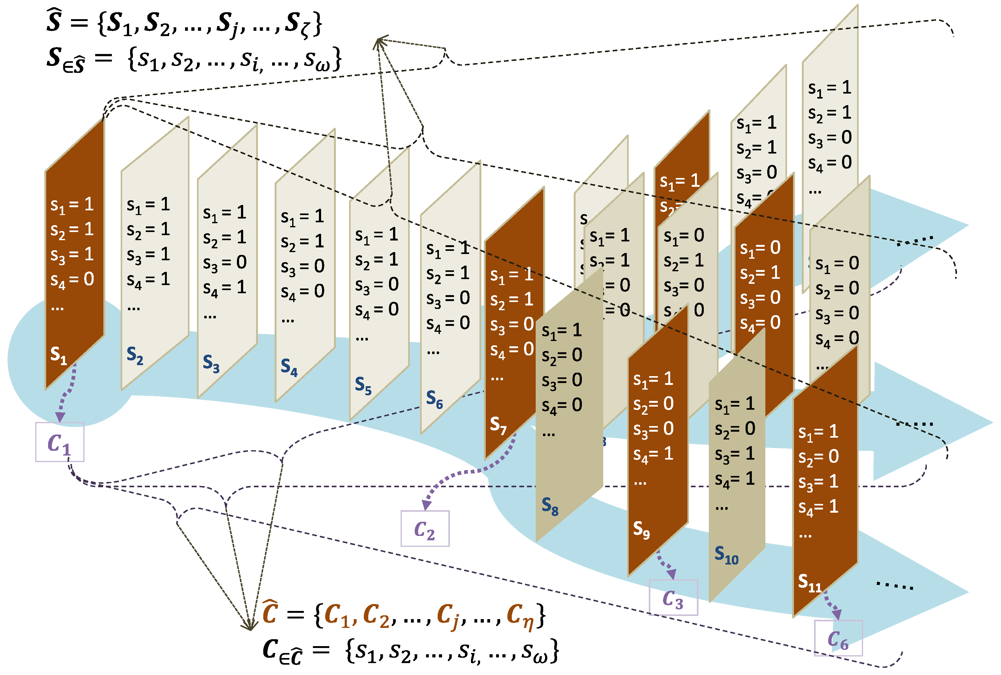
This paper proposes methods for modeling and reasoning contexts that can achieve full automation. In our definition, contexts are modeled by the sensors, which are attached to the entities, including objects, humans, and other built-environment artifacts. Based on the context models, the recognition process proceeds to reason a context by analyzing the given sensor data. Since both modeling and reasoning processes need to manage sensory data, it is critical to build a context in an efficiently organizable and easily manipulable structure. In our approach, we developed a method in which a well-organized context model is built by analyzing sensory data that describe the status of contextual entities. To model this context structure, we considered two key ideas. The first idea comes from the observation that most sensors triggered in the same context are somehow interrelated. The second idea comes from the observation that there are sensors that are significant and conducive to specific contexts. This observation raises the possibility of logically dividing a whole sensor dataset into groups, each of which contains data from inter-related sensors. Since each of the divided groups is likely an own-context, by virtue of the two aforementioned observations, it is important to logically divide a given dataset accurately, which, in turn, requires that we properly find interrelated sensors and their data. We address dividing and searching methods for building context models in more detail in the rest of this paper.
The proposed approach proceeds in two phases: First, context models are built, and then a present context is determined from the context models. In the first phase, the context models are inferred from a collection of obtained sensor datasets under supervised learning. For the inference process, we utilize three machine learning methods along with statistical analysis: K-means clustering, a conditional probability table (CPT), and principal components analysis (PCA). The second phase begins after the context models are successfully established. In this phase, we compare the current state space to all the context models and choose the context that is most similar to the current state space. The similarity is calculated by two distance methods: Euclidean distances and cosine similarity. To systematically and algorithmically facilitate the two phases of our approach, we introduce and utilize a high-level contextual structure, called a context graph, to be utilized in developing and using (reasoning) the context models.
The modeling and reasoning process may lead to privacy and security issues for smart-space systems and their users. In smart spaces, the most used and very efficient sensing devices are cameras, which can capture the data of any user and/or objects seen in the camera range. The data may contain more information than that which must be obtained; there may be someone who does not wish to be sensed or private objects that must not be digitalized. At-home settings, which are more private and secured, require further caution when cameras are used [
16]. For these reasons, and out of an abundance of caution, only data obtained by means other than cameras are used in this paper.
We organize this paper as follows. In
Section 2, we describe existing work related to context-awareness computing, context modeling, and reasoning methods.
Section 3 introduces the design of the proposed context model and context graph, which provide a fundamental formalism to our approach. The principles of the proposed approach for modeling and reasoning contexts from a real-world situation are presented in
Section 4. Experimental validation and case studies follow in
Section 5. Discussions and conclusions for this research are presented in
Section 6.
4. Principles of Context Reasoning
In context awareness computing, reasoning a context is functionally the same as finding the next context in the present context. Thus, our approach aims to discover the next context with respect to the present context, and the current state space, . The main procedure for reasoning is that, in a given , happens, and then it becomes a next context, , which is found from the next possible context, , if is sufficiently similar to . Our approach follows this procedure, and all the methods in our approach are designed to find the next context.
4.1. Overall Approach
The reasoning process is fundamentally event-driven since it proceeds whenever a sensor event occurs. The sensor event is caused by resident activities or the movement of objects in the space, and then changes a state space. Assuming that the current context is
, if the reasoning procedure qualifies the changed state space as the next context
, the transition into
is indeed performed, as shown in Algorithm 1. Otherwise, if the algorithm fails to find such
the current context remains, and the algorithm waits for the next change in the state space. Algorithm 1 runs in two phases: (1)
MODELING and (2)
REASONING.| Algorithm 1. Context Reasoning Main |
|
- 1.
- 2.
- 3.
- 4.
- 5.
- 6.
- 7.
- 8.
//transition to - 9.
- 10.
- 11.
|
4.1.1. MODELING
The initial step for reasoning contexts is to establish a context graph
with a given set of state spaces
which is formed from training datasets.
is built by applying the statistical analysis method of sensor datasets [
4]. The statistical analysis method runs in three main phases. First, the dataset is analyzed by a conditional probabilistic table (CPT) based on Bayesian networks and estimates the number of contexts, that is,
. Then, the dataset is clustered into
contexts by applying
-means clustering. Thirdly, conditions for entering a context are discovered by utilizing principal components analysis (PCA). PCA is a way of finding important components and reducing the dimensions of a given dataset by projecting it into the lower dimension [
39,
40]. The use of PCA helps to find the most important sensors for a given context and optimizes both the context modeling and reasoning, which will be explained in detail in the reasoning step.
Once
is established, the current state space
and the present context
are initialized.
is simply configured by the current status of sensors. Initialization of
is performed by the Algorithm 2. The purpose of the algorithm is to find an initial present context
which has the highest similarity with
.
| Algorithm2. Initializing Context |
|
- 1.
- 2.
- 3.
- 4.
- 5.
- 6.
|
4.1.2. REASONING
When the current state space
changes due to a sensor event, an attempt is made to reason a context that is most similar to
as shown in Algorithm 3. If a proper context model is found, it becomes the new present context
. As in Algorithm 2, the similarity between
and each target context
is calculated. The proposed algorithm can reduce the number of target contexts when calculating the score due to
. By the definition of
, since
is followed by
of
, only contexts in
are considered in the reasoning process. If the reasoning process is unable to find any context model, that is,
is empty (line 7 in Algorithm 1), it does not transition to the next context, and the current context
continues.
| Algorithm 3. Reasoning Context |
|
- 1.
- 2.
- 3.
for - 4.
- 5.
- 6.
- 7.
- 8.
.
|
Differing from Algorithm 2, which selects any context and declares it as , more consideration is needed to discover the possible next contexts . If a context is too different from , it must not have a chance to become . In some cases, contexts in have too low a similarity and should not be any context. To address the cases, a context requires filtering by a threshold , which stands for a particular similarity grade. We will introduce the reasoning methods and define in the next section.
4.2. Context Graph Building Steps
The approach proceeds in three steps, each of which utilizes a statistical method. First, the number of contexts is decided by a conditional probability table (CPT), and then meaningful and representative state spaces are defined as contexts by K-means clustering. Lastly, important sensors, which are related to each context, are discovered by using principal component analysis.
4.2.1. Deciding the Number of Contexts
To find the number of contexts, we first capture the probability of the consecutive occurrence of each pair of different sensors in the datasets. The idea is that sensors in one context are related and, thus, the occurrence probability is fairly high [
41]. In other words, if the occurrence probability of a pair of sensors is low, the sensors are not in a context. This probability can be accurately calculated from the frequency of occurrence of consecutive sensor events. These conditional probabilities are arranged as a
table (
being the number of sensors), which is called the conditional probability table (CPT).
Figure 3 shows how to decide on a pair of consecutive sensor events and how to build a CPT.
CPT is used as the probabilistic fingerprint of the entire dataset. A pair of sensor events with high conditional probability usually contains sensor events that are related and associated with each other. They could belong to the same context and, therefore, are highly likely to occur together in this order. On the other hand, if the pair has low conditional probability, its sensor events are considered to be unrelated and would rarely occur together. A pair of sensor events with low probability indicates the end of one context and the start of another. Therefore, we divide the dataset between sensor events and if the conditional probability of and satisfies the condition , where is a parameter that represents the extent to which relates to . We set to 0.5 in the experiments. Using this method, we divide the dataset into groups, which are considered the number of contexts.
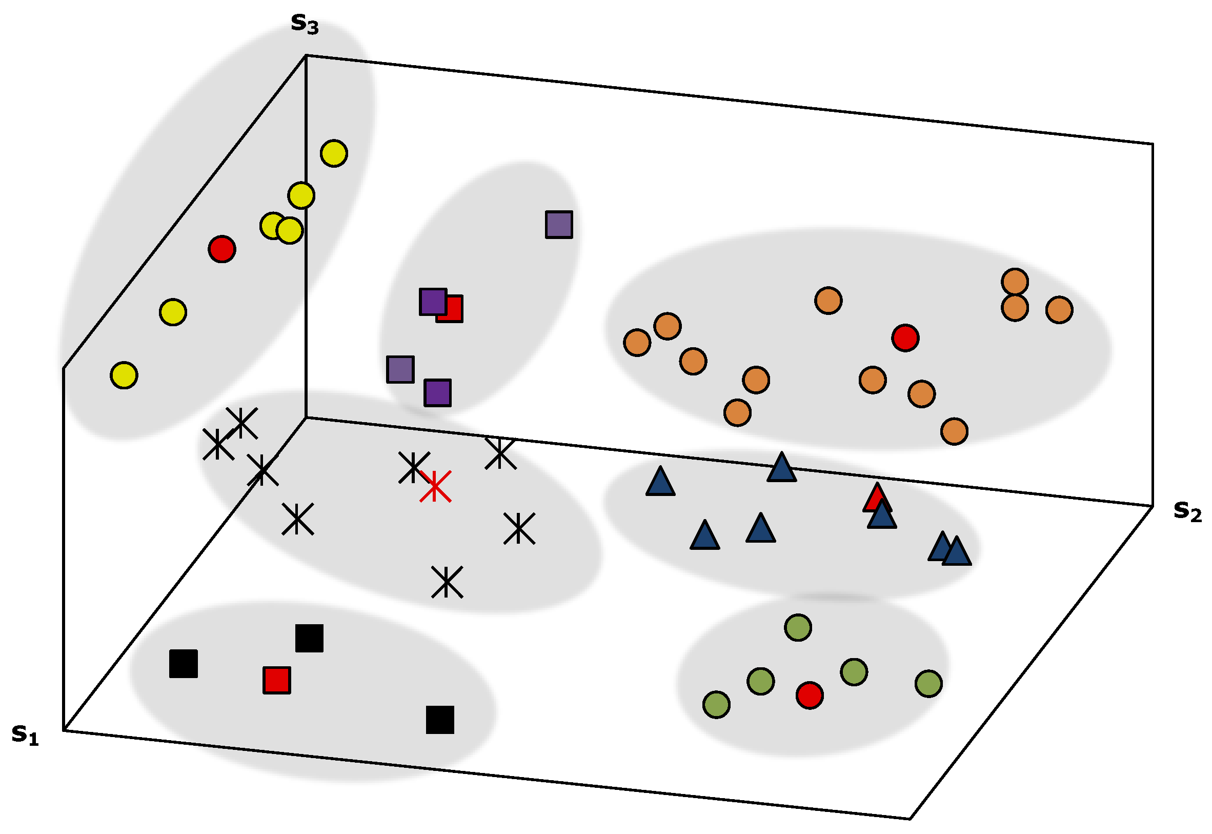
4.2.2. Defining Contexts
We observe that a meaningful state space is sufficiently distant from other meaningful state spaces but could be close to other relevant, yet non-meaningful, state spaces. To find out which state spaces are meaningful, all spaces are partitioned into
clusters, in which each state space belongs to the cluster with the nearest mean. Therefore, the universal set of state spaces
is divided into
, where
is a state space and
is a cluster of state spaces. Each cluster
minimizes the sum of distances between the within-state space and the mean, according to the following formula:
where
means a state space in cluster
. After
is classified into
clusters, cluster centroids are considered meaningful state spaces and are candidates for contexts. Note the number of contexts obtained from the previous step.
Figure 4 illustrates an example of how contexts are clustered and chosen from a set of state spaces.
4.2.3. Discovering Context Conditions
The centroid in context is representative and meaningful but has insufficient information to define the context. We observed that multiple sensors usually contribute to beginning a context. Principal components analysis (PCA) can discover these important sensors. Once we find the relevant sensors via the stochastic analysis of the sensors’ high-dimensional data, the original dataset can be projected onto lower-dimensional data. The process is repeated for each cluster, and the remaining data are used to build context conditions.
Principal components are sensors that show definite variance patterns that explicitly express a change of states. To discover these sensors, we should understand the pattern in which the dataset is scattered. For this, a matrix of covariances (
cov) is calculated first. In a
-dimensional dataset, covariance
cov is calculated by Equation (7):
where
and
stand for the set of sensor values in
th state space and
th state space, respectively.
belong to the same context. Since the maximum number of state spaces in a context is
, the total covariances establish a
covaraince matrix
, shown in the Equation (8):
From the covariance matrix
, we calculate the eigenvectors, which characterize the square matrix as linear equations, each of which can transform the matrix onto a new axis. Eigenvalues then measure how well the sensor data are scattered. Eigenvectors and eigenvalues are calculated by the following condition:
where
is the eigenvectors and
is the eigenvalues. As
is a
matrix,
is also a
matrix, that is
eigenvectors exist. Each eigenvector has its own eigenvalue; therefore, there are
eigenvalues in
:
where
is an eignevetor with
components.
Next, we choose the eigenvectors with high eigenvalues as principal components. The challenge is in determining the threshold for which eigenvalues are high enough to be acceptable. We propose the threshold
for the average of eigenvalues of selected eigenvectors. In our approach, the eigenvectors are sorted by eigenvalues in descending order; then, eigenvectors with values that exceed
are chosen. Eigenvectors satisfying this condition establish a feature matrix
:
where
,
,
is an eigenvalue of
. With a feature matrix
, a given dataset is transformed into lower-dimensional data with
sensors. The conditions for a context are a collection of sensor values in the lower-dimensional data.
4.3. Context Reasoning Methods
To reason a context, the similarity between and each possible next context is considered by calculating . Since the state space and context conditions are vectorized by the status of sensors, can be computed by two methods, as shown below.
4.3.1. Similarity Based on Euclidean Distance
When the distance is within a fuzzy threshold,
which specfies a range for the condition of
, signifies no difference between
and
; hence,
becomes the next context. Note that
is context-specific; thus, each context has its own value. This is obtained by averaging the distances from each state space to context during the initialization step [
4]. Some conditions may be defined with a range of values, instead of one value. In this case, to apply Euclidean distance, the range is represented by a median of the range. For instance, if the range of sensor’s values is from 0 to 5 in an integer, its median, which is 3, is used to compute the Euclidean distance. The Euclidean distance is calculated by the following Equation (11):
In Equation (12), stands for the status of sensor in the current state space , and stands for the status of sensor in the possible next context, .
If the distance is below
, the
is considered to possibly be the next context. On the other hand, when the distance is greater than
, there is no chance for
to become
. The similarity is calculated and compared for all
which satisfy the distance condition, that is,
:
If none of verifies the condition, the current state space cannot not be any of the contexts, therefore no change in context occurs.
4.3.2. Similarity Based on Cosine Similarity
Dissimilar to the Euclidean distance, which values the distance between the end points of two vectors, cosine similarity verifies the appropriateness of the angle between two vectors. The
is calculated as follows:
As the cosine of two vectors increases to 1, the vectors are considered more similar. All of in must be within the threshold for the condition of to be considered the possible next context. Failure to find such delays the transition to any possible next context.
fits when finding the similarity of state spaces with Boolean-stated sensors, such as sensors generating two statuses of 0/1 or On/Off. In other words, when the change in sensor status is monotonous and, thus, the magnitude of vectors and is stable, the Euclidean distance can be applied. However, this is not applicable when the status in the sensors is non-Boolean and generates values within certain ranges since the magnitude of vectors can significantly change. For the state spaces containing those sensors, is used.
In the reasoning methods above, each vectorized element is individually calculated. As the given space is extended and the state space is scaled with more sensors, the computational complexity greatly increases and affects the performance in reasoning contexts. Since the number of sensors matters, it is critical to reduce the size of the sensors. To achieve this goal, we utilize PCA and reduce the dimension of the dataset for faster computation when calculating similarity. Note that the PCA is applied regardless of the similarity method.
5. Experimental Validation
Automation reduces time and effort for modeling the structures of a process and avoids potential errors when manually configuring a process. However, an automated process might downgrade performance due to the lack of an ability to catch and handle unexpected exceptions. The validation point for an automation-enabled approach is to consistently show results that are as good as those produced by non-automated approaches in various cases. Therefore, we performed experimental validation with case studies to show whether these contexts are reasoned by our approach without violation. In the experiment, we conducted a reasoning process for a day-long scenario and evaluated whether a set of appropriate contexts was sequentially recognized. The contexts located within the set are considered as a contextual schedule, notated by (). Thus, the validation aimed to analyze the and decide whether this is reasonable and feasible. For our validation, we defined two measurements: Fidelity and Feasibility. Fidelity is used to measure the degree of reasonability of a , and Feasibility is used to terminologically describe whether the is at all possible by Fidelity. In short, Fidelity generates numeric measurements, and Feasibility divides the range of Fidelity to particular categories. The categories of Fidelity will be introduced after explaining how to calculate Fidelity. If a has a high Fidelity, it could be said to happen with high probability and be categorized as “good” Fidelity. We verbally describe it as being feasible or possibly feasible.
Our approach was validated by showing how many are feasible. For this goal, we conducted the following steps:
- 1.
Preparing datasets: we built context models and context graph by analyzing sensor datasets. In this step, we obtained datasets from real-world scenarios, which are used as training sensor datasets for forming . Note that each sensor dataset is formed in a collection of state spaces, . Then, we prepared more datasets as testing sensor datasets, which were used in the Evaluation step. Each testing sensor dataset also follows a form of .
- 2.
Testing an approach: we reasoned the testing sensor datasets and obtained context schedule . Note that we had to test each dataset; thus, there were multiple , which were used to calculate fidelity.
- 3.
Evaluating context schedules: we evaluated whether each context schedule obtained in the testing step was feasible. In the evaluation, we analyzed that a could be found along with context graph built in the preparing step. If the could be located, we could validate that the reasoning process was flawless. If we failed to find it, we considered two reasons. First, the was not feasible, and this meant the reasoning process had flaws. Second, the was not accurately established, which inferred that the modeling process was errored. Next, we will explain the conditions for evaluation algorithms.
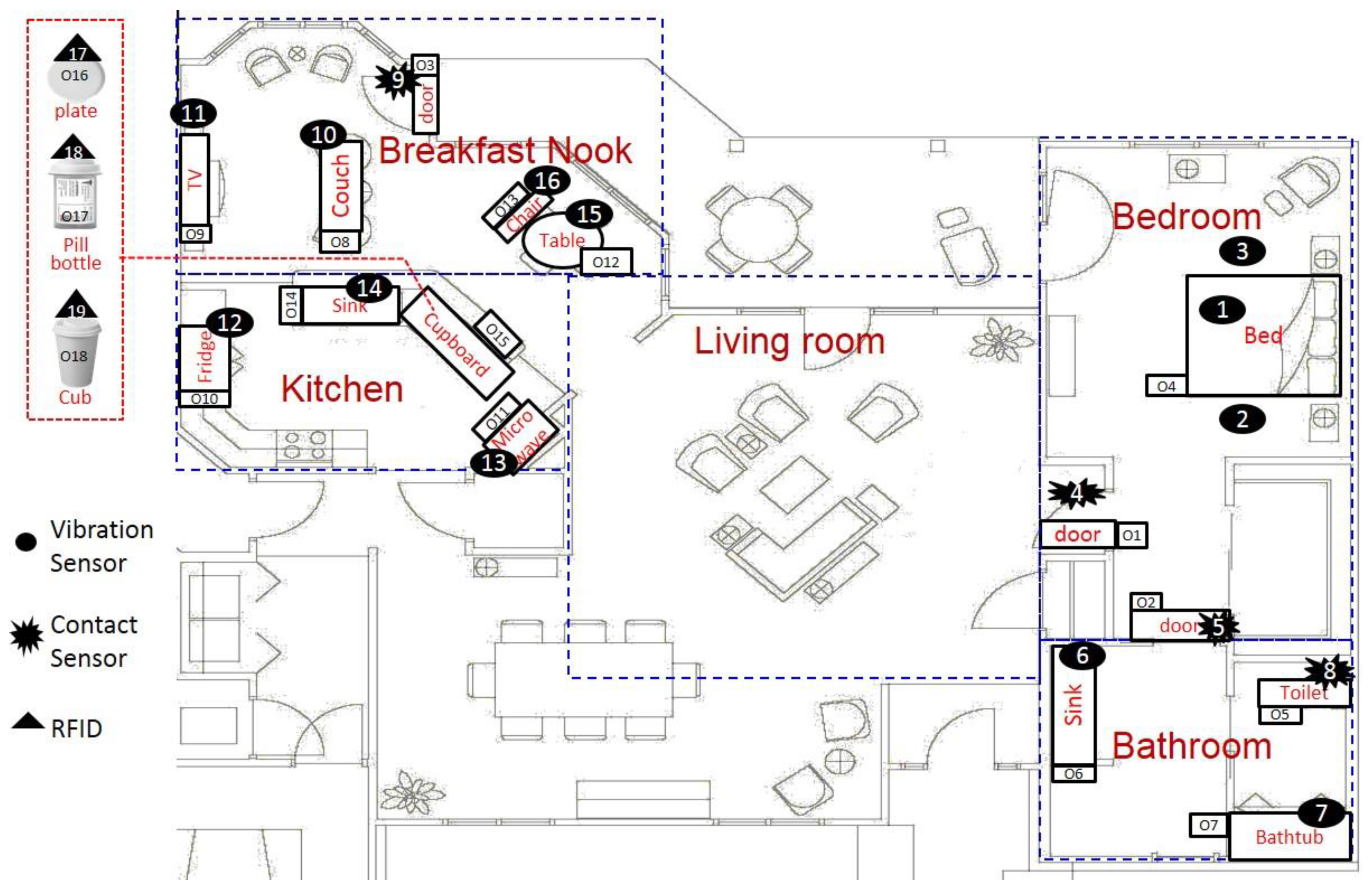
First, the training sensor datasets were collected for 11 days in the Gator Tech Smart House (GTSH) [
42]. The datasets captured the status of 19 sensors, which were deployed on 18 objects, while 8 activities were performed by 2 volunteer testers. The floor plan describes where the objects and sensors were placed, as shown in
Figure 5. A daily living scenario in which 8 activities were performed was proposed in [
43].
Next, we used the Persim 3D simulator [
43], which generates the testing sensor datasets. Persim 3D simulates pre-defined context models and a context graph
based on a context-driven approach, and then synthesizes different datasets. We obtained 11 testing sensor datasets and generated 11 context schedules
using our reasoning process. We then evaluated the 11
and proved that they could be discovered in
. For a more accurate evaluation, we proposed the following conditions and proved that they all were met in order:
Condition 1. Condition 1 allows us to filter out cases of single contexts in which there is no transition of contexts; thus, the reasoning approach fails to find another context. In this case, a daily living scenario starts and ends in the same context without any transitions. This is considering the fact that the reasoning approach does not work properly. In our experiment, there was no testing sensor dataset that could not pass this condition. However, this does not guarantee that is feasible, even though it consists of more than two contexts, and thus passes this condition. This condition is not enough to catch exceptionally occurring contexts, which may be accidentally sensed by sensor errors. For this reason, needs to satisfy the next condition:
Condition 2. Condition 2 restricts to accept only the most likely occurring context schedules . This proceeds with context graph which was made in the preparation step. Recall that is built in a directed graph, which describes all transitions between contexts. This means that can reveal various context paths, each of which is considered a . Each is evaluated by its probability of occurrence, denoted by . Note that the low probability of occurrence of an event means that it rarely or never occurs. Thus, we can infer that a with a low probability rarely occurs and, hence, it should rarely be reasoned.
The
Fidelity and the
Feasibility of
is measured based on the probability. For this goal, statistic models were defined as follows: First, we calculated the join probability distribution of
based on use of the Bayesian network (BN) and conditional probability table for contexts. BN-based probability
of
is computed by Equation (9):
In Equation (9),
calculates the conditional probability of two distinct contexts,
followed by
presents the probability for occurrence of a given
however, it is not enough to measure the
Fidelity and the
Feasibility. Even if a
has a high occurrence probability but it rarely occurs, it could be considered as an exception or an error, and thus should have a low
Fidelity. To resolve this,
Odds for
is calculated by Equation (10).
stands for the probability of a
, and denotes how often the
occurs. In this experiment, it can be computed by the frequency of occurrence of a
over 11, the number of total training (or testing) cases.
The
and the
are used for computing occurrence probability,
.
is used for determining
.
is obtained by calculating an arithmetic average of
for all given
. In our experiment,
was 0.301 for the training datasets.
In the evaluation step, we repeated the entire process with testing datasets, which are generated by Persim 3D, and we obtained , , and . Then, we conducted the validation process by computing Fidelity and deciding Feasibility. Fidelity is measured by the ratio of the of the testing sensor datasets over OPT. If the is below , it means that the is unreasonable and irrational to occur. The maximum Fidelity is 100%, which implies that the of the testing dataset occurred in the same probability.
However, even though the
Fidelity of a
is not 100%, it is hard to decide whether it is not yet reasonable. Since
and
were calculated by statistical analysis based on probability distribution, this may be adjusted as more training datasets are collected and used. Therefore, we categorized the
Fidelity into three states, which increased the flexibility of evaluation. We defined the
Feasibility states as falling into the three
Fidelity categories, as shown in
Table 1. A
with 100%
Fidelity is classified into the category
Feasible. If the
Fidelity of a
is below 100%, yet considerably low, we assume that the
may be feasible in certain conditions, and thus accept it even though it is not guaranteed to occur. In our experiment, we analyzed the training datasets to determine the proper range for the category
Possible by using Equation (17) and obtained 64%:
In Equation (17), stands for the context schedule obtained from an ith dataset, and is a ratio representing how many context schedules are beyond the average. This is calculated by the number of whose occurrent probability is above , over the total number of .
The
OPT of the 11 testing sensor datasets is shown in
Table 2. The
Fidelity score of six datasets shows 100%, which means that they are
Feasible, and those of the other three datasets are categorized in the
Possible state
which means they might be acceptable. Hence, we consider that nine datasets are feasible. On the other hand, the
Fidelity score of two datasets (no. 4 and 9) are not in the feasible or possible range, showing that they are below the minimum possible score, which is 64%. This means that the contextual schedules
of the datasets have very low conditional probability and thus very rarely occur. In summary, the proposed approach’s overall success in reasoning contexts is 81%.
6. Discussion
In this paper, we proposed an approach for the automation of modeling and reasoning of contexts in smart spaces by stochastically analyzing the sensor data. Traditionally, and still in many applications, contexts are semantically and manually defined and configured using ontology-based modeling methods. Those methods enable well-organized structures for contexts and can be applied in human-centered machine and human-oriented smart spaces since they are readable and associable for human users. However, manual configuration requires human efforts and cannot be an optimal solution in this pandemic, which demands fewer physical contacts or assistance. The main contribution of our approach is to reduce humans’ efforts in defining contexts and recognizing a current context and enables automation of the process. To achieve this goal, we employed a mathematical and statistical analysis of the data collected from sensors attached in smart spaces. First, we utilized a conditional probability-based analysis, K-means clustering, and PCA to build context models. In the processing used to determine a present context, we applied Euclidean distance, cosine similarity, and PCA. In all processes, when defining and recognizing a context, PCA was used to filter out sensors that had no contribution or minimal contributions and, eventually, to reduce the computational complexity.
As shown by experiments with positive performance results, our approach was shown to be validated and applicable. In the future, we plan to enhance the approach, which can dynamically adjust context models, which were already built while running a reasoning process. The current approach is generally based on the supervised learning method, and thus establishes a static model, which will be used to reason a present context. It is possible to fail to determine any context if the current state is very new or unexpectedly occurs due to forces external to the smart space, such as a natural disaster or the occurrence of unknown diseases. To address this issue, our future research will examine unsupervised and more dynamic learning methods and assesses their success in recognizing present contexts without training, and then modify the context models. The enhancement will include research to discover unknown contexts in the reasoning process, define them, and update the context graph. A related approach, which is equally important, is avoiding “impermissible contexts”, which are known a priori but are not permitted to occur [
44]. We will also develop methods to optimally map the present context to the most relevant services for the human residents in the space. This would improve real-world applications so that they work without training steps.


