Abstract
This paper studies the behavior of a Euro 6 diesel engine tested under dynamic conditions corresponding to different real driving emissions (RDE) scenarios. RDE cycles have been performed in an engine test bench by simulating its operation in a long van application. A computer tool has been designed to define the cycle accounting for different dynamic characteristics and driver behaviors to study their influence on CO2 and pollutant emissions, particularly CO, THC, and NOX. Different dynamic parameters have been established in terms of power, torque, engine speed, or vehicle speed. Additionally, a tool to estimate the emission of an RDE cycle from steady-state maps has been developed, helping to identify emission trends in a clearer way. Finally, the conclusions suggest that driving patterns characterized by lower engine speeds lead to fewer emissions. In addition, the analysis of RDE cycles from stationary maps helps to estimate the final tailpipe emissions of CO2 and NOX, offering the possibility to rely on tests carried out on engine test bench, dynamometer, or on the road.
1. Introduction
Pollutant vehicle emission and carbon dioxide limits are becoming increasingly restrictive. In Europe, the certification limits of carbon monoxide (CO), nitrogen oxides, particulate matter (PM), and the sum of NOX and total hydrocarbons (THC) for diesel engines have been reduced in large proportions since Euro 1 [1] to the current Euro 6d [2], as Table 1 shows.

Table 1.
Pollutant vehicle emissions from Euro 1 to the last Euro 6. * In the case of NOx, since the first limit was established (Euro 3).
Nowadays, the world is facing the impact of climate change, the last six years being the warmest on record [3]. To achieve the challenges proposed in the climate change conference held in Paris 2015 [4], the concept of carbon footprint is of great importance, especially for greenhouse gases (GHG) emissions management [5]. Major developments in renewable energies [6] have been occurred to reduce GHG emissions although additional efforts are required from key sectors such as transportation. In this regard, the European Union (EU) has established stringent standards which have been reflected in the 443/2009 [7] regulation. This directive establishes that the EU fleet-wide average emission target for new cars must be 95 g CO2/km from 2021. Later on, the EU decided to reduce this limit by an additional 15% from 2025 and 37.5% from 2030 through regulation 2019/631 [8].
Along with increasingly restrictive CO2 emission limits, a change in the type-approval cycle has also been set and the New European Driving Cycle (NEDC) became obsolete [9]. Instead of NEDC, two new cycles were established to represent real driving conditions accurately. First, the World Light-Duty Test Cycle (WLTC) was designed from “real world” driving data [10], and second, the Real Driving Emissions (RDE) cycle appeared for the first time in 2016 [11]. Both WLTC and RDE cycles reflect greater accelerations than NEDC, which produce an increment in the engine operating range [12,13], entering the high torque and speed region of the engine map. Concerning the methodology to perform the tests, a chassis dyno is used to perform WLTC [14], while RDE must be carried out on road [15].
The newest RDE regulation [16] dictates a series of guidelines to carry out the test. In case any of the requirements were not fulfilled, the cycle would be considered invalid. Although the regulation is very extensive and detailed, the number of possible cycles is infinite so different tests can have an important dispersion in terms of pollutant and CO2 emissions. Therefore, factors such as traffic, weather conditions, altitude, route typology, road grade, and driver behavior [17,18] have a great influence on the cycle results [19,20]. Even repeating the same trip, large differences between different cycles can be found [21]. Moreover, some studies combine experimental on-road data with numerical analysis to assess the impact of the stop/start system, vehicle mass, drag coefficient, and different aftertreatment system layouts [22].
One methodology to analyze engine operation in RDE-like conditions consists of performing cycles in a dynamic engine test bench instead of directly in the vehicle. In this way, since the tests have been performed under highly controlled operating conditions, the intrinsic engine response can be analyzed with greater reliability, since the uncertainties caused by traffic, temperature, or driver behavior are eliminated [23]. It is possible to find similar studies in literature aimed to improve the reproduction of the flow conditions on road and to be able to perform cycles on a chassis dyno [24,25,26] which also helps to simulate a vehicle in an engine test bench. Furthermore, it is added that, although portable emissions measurement systems known as PEMS are being improved [27], they have smaller accuracy than a stationary system [28,29]. In no case has any complete comparative RDE study been found as has been carried out in this research.
In this paper, six different cycles have been analyzed, all consistent with RDE regulation but having different dynamics, and were performed during the experimental campaign. The aforementioned methodology has been always applied, which allows rigorously analyzing the data registered from the tests. The first one replicates an on-road cycle and will be used for baseline comparison. A second one was designed combining several WLTC dynamic phases. The last four were defined using a computational tool considering different dynamic conditions. Concretely, with the last two cycles, a study analyzing two different driver behaviors has been also performed, which could not be carried out on road in a consistent and repeatable manner. The data from the aforementioned cycles were analyzed in detail to relate cycle dynamics and engine operation.
2. Materials and Methods
2.1. Methodology
In order to be able to compare real cycles accurately, an engine test bench was employed to reproduce the conditions of every proposed test. In this way, the inherent uncertainties of on-road tests are eliminated and a common framework for comparison is established. The test bench hosted the engine, together with the following facilities.
2.2. Test Bench and Engine
The test bench hosts the engine, together with the following facilities:
- SCHENK DYNAS3 asynchronous dynamometer, which imposed the brake of the engine by simulating the corresponding resistance force along with the real driving cycles. The resistance force applied by the brake is considered aerodynamic, friction, and inertia forces that would be exerted on the vehicle.
- Type K class B thermocouples.
- Kistler 4045A5 piezoresistive pressure sensors.
- Horiba MEXA-7100 gas analyzer, which measured volumetric concentrations of O2, THC, NOX, CO2, and CO at the exhaust tailpipe. CO2 concentration was also registered at the intake manifold, downstream of the EGR junction to estimate the EGR rate.
- AVL 439 opacimeter, to obtain the particulate mass, the opacity has been measured, and later it was traduced to soot density [30] through Equation (1).
In addition, k is calculated with Equation (2):
where:
- L = measuring length.
- N = opacity (%)
After calculating the soot density, it is possible to obtain the PM mass flow, through the exhaust mass flow.
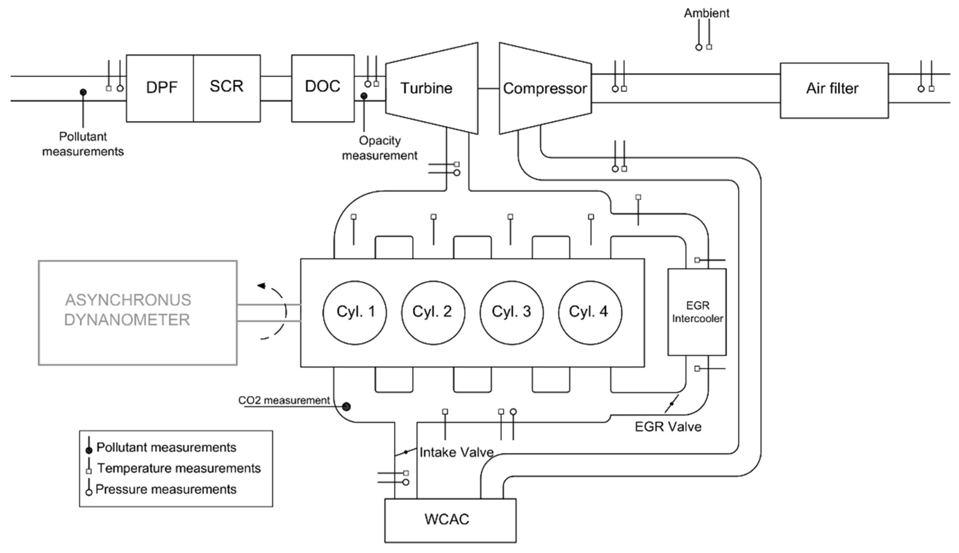
A 2.18 L displacement, 126 kW Euro 6 turbocharged four-stroke diesel engine of four cylinders has been used to perform all the tests. The engine was equipped with a high-pressure exhaust gas recirculation system which also has an intercooler before the engine intake. To control the intake temperature, a water charge air cooler (WCAC) is submerged in a coolant tank and a PID controller regulates the coolant flow to keep the required air intake temperature.
The aftertreatment system was composed of a diesel oxidation catalyst (DOC) responsible for oxidizing THC and CO, and a diesel particulate filter (DPF) to minimize the PM emissions. Considering that the DPF requires periodic regenerations, a specific cleaning procedure was performed between two consecutive cycles. This strategy complemented the passive oxidation promoted by cerium dioxide added to the fuel.
Finally, a selective catalytic reduction (SCR) to reduce NOX emissions was integrated into the exhaust line. Nevertheless, the AdBlue injection was deactivated in all tests. Therefore, although the gas analyzer was placed downstream of the aftertreatment system, raw NOX emissions were monitored.
The engine layout and pressure, temperature, and polluting sensors installed in it are shown in Figure 1 The Acquisition frequency was always 1 Hz (as RDE regulation imposes) for all the pollutant emissions, dynamic variables, temperatures, pressures, and mass flows.
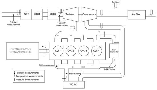
Figure 1.
Engine layout.
2.3. Simulated Vehicle
The vehicle simulated in the engine test bench was a van as it commercially corresponds to the tested engine. Gearbox and vehicle characteristics were defined in the software to perform the driving cycle simulation in the test bench. Table 1 shows the mechanical characteristics of the vehicle.
In order to calculate the instantaneous forces acting on the vehicle along time, Equations (3) and (4) were applied [31], where FAero is the aerodynamic resistance force, Cx is the transversal coefficient, A is the section of the vehicle, is the air density, is the vehicle speed. In addition, FRolling is the rolling resistance force, where is the rolling coefficient, M the vehicle mass, the gravity acceleration, the road grade. The values of the different coefficients can be found in Table 2.
Table 2.
Vehicle characteristics.
The required power ) to be supplied by the engine was calculated according to Equation (5), where corresponds to the instantaneous vehicle acceleration:
3. RDE Cycles Description
Six different cycles were defined to carry out an evaluation of the emissions and the consumption of the engine in different driving conditions. All cycles met the conditions required by the current Euro 6d regulation to be considered valid. Given the vast number of cycles that can fulfill the requirements, these were chosen in such a way that, maintaining similar typologies, the effect produced by the specific modifications implemented in each of them were comparable.
In this study, the maximum engine speed was set along with the gear shifting, representing different driver behaviors under the standard field of diesel engines. Table 3 shows the maximum engine speed at which the shifting sequence occurs for each RDE cycle.
Table 3.
Maximum engine speed limits for each gear.
3.1. RDE 1
This cycle was obtained from on-road driving in Valencia (Spain) [14]. Using the data obtained from this test, it was possible to transfer its characteristics to the engine test bench. In particular, a vehicle model was used to calculate the instantaneous effective torque and engine speed considering the vehicle speed profile, the vehicle, and gearbox characteristics, and the driver behavior. These two parameters were used as inputs in the engine test cell.
3.2. RDE 2
The second cycle performed was obtained combining different WLTC segments to meet RDE requirements. WLTC represents real driving conditions, although Euro 6 regulation imposes that it must be performed in a chassis dynamometer. It is expected that WLTC will also be used in the next Euro 7 regulation.
In this case, WLTC phases in which the vehicle speed is less than 60 km/h were used to generate the urban zone, phases with vehicle speed between 60 and 90 km/h were applied to build the rural zone, and phases characterized by vehicle speeds over 90 km/h were considered to define the motorway zone. As WLTC is much shorter than the RDE cycles, several WLTC parts were mixed and repeated. After obtaining the speed profile, it was combined with the remaining data related to vehicle, gearbox, and driver to obtain the required torque and engine speed that allowed to meet the instantaneous vehicle speed setpoint.
3.3. RDE 3, 4, 5, and 6
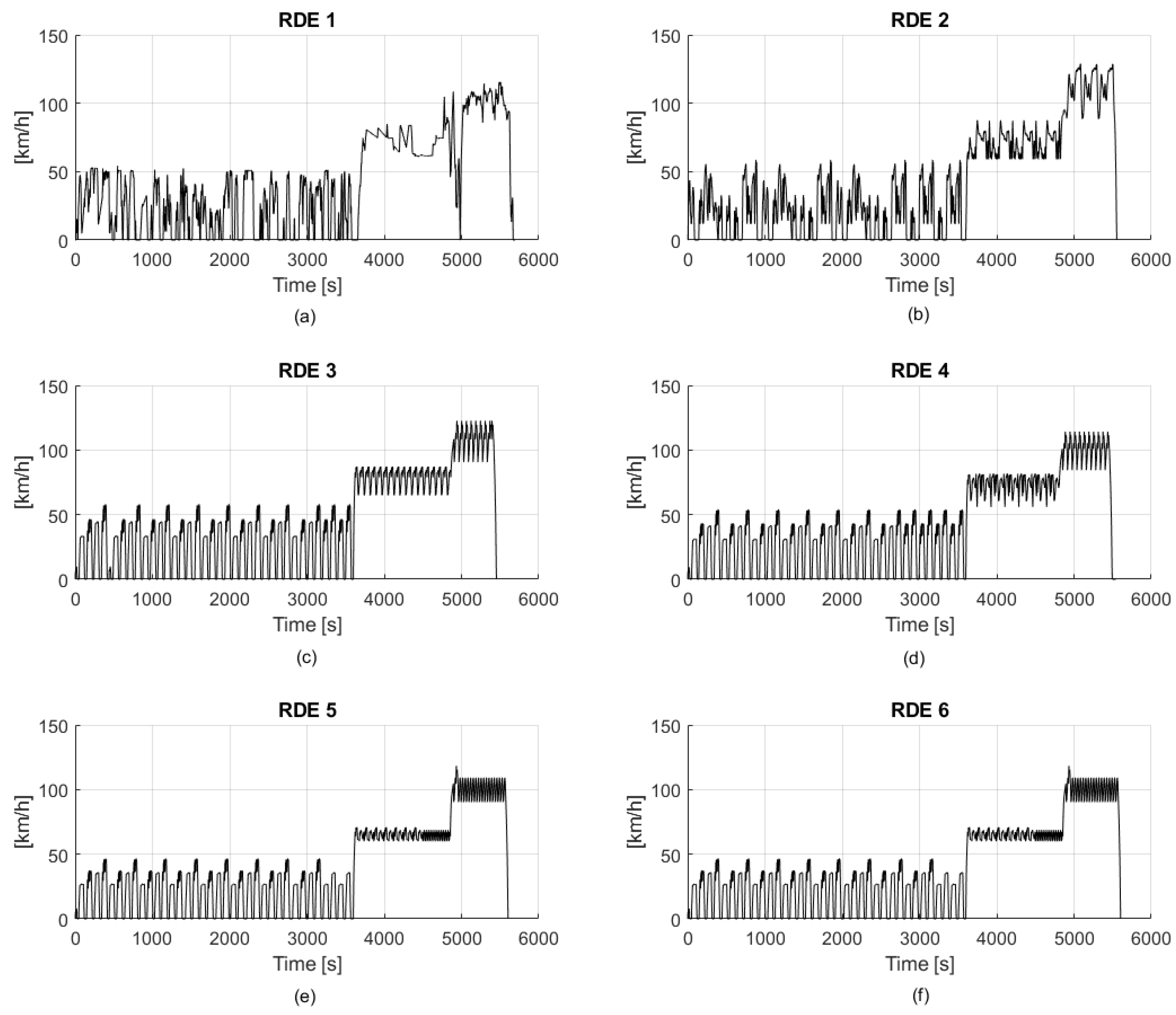
The last four cycles were obtained using the same methodology using a computational tool designed to generate RDE cycles. The function selects different speed profiles, with different vehicle speeds and accelerations, to fulfill the regulation requirements combining standard real driving segments. As a result, cycles with different dynamic demands, durations, and other characteristics are obtained. The user can choose in the software the number of times that every phase, which is characterized by different engine load conditions, is repeated. Consequently, depending on the number of dynamic phases, the cycle generated is more or less loaded. With this procedure, torque and engine speed were finally determined in the same way as the previous cycles. All the RDE vehicle speed profiles are shown in Figure 2. All the cycles presented a certain repetition pattern in the route. In the urban zone, it could be like repeating the same circuit in a certain city, provided that the conditions of traffic, driving behavior, and traffic lights do not affect it. This approach was also applied in the rural and motorway areas, where the same conditions could be reproduced in a highway without traffic and that the driver replicated the speed conditions imposed. Using this tool, different types of routes, driver behaviors, etc., can be examined, reducing economical costs and uncertainties from on-road testing.
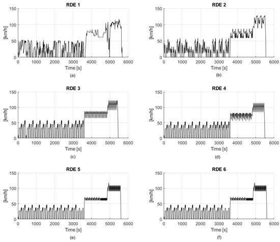
Figure 2.
RDE 1 (a), RDE 2 (b), RDE 3 (c), RDE 4 (d), RDE 5 (e), and RDE 6 (f) vehicle speed profiles.
- RDE 3: This cycle presented the lowest duration but the highest average vehicle speed in every zone. This cycle was also characterized by a similar proportion of high and low loads.
- RDE 4: In this case, the previous RDE 3 was taken as a reference. The objective of RDE 4 was to generate a more dynamic cycle in the rural zone. This cycle was also less loaded being the average vehicle speeds in urban and motorways zones are lower than in RDE 3.
- RDE 5: The objective of this cycle was to generate a less loaded and dynamic cycle than the previous ones. In order to achieve that, phases with low dynamic demands were chosen. As observed in Figure 2, the differences in vehicle speed were reduced for the rural and motorway zones compared to other cycles.
- RDE 6: This last cycle was obtained with the same vehicle profile as RDE 5 with the driver behavior as the only difference. In this case, the gear shifting sequence was modified, advancing it to obtain a lower engine speed profile.
Figure 2 shows noticeable differences between RDEs 1 and 2 compared to RDEs 3 to 6, despite the patterns of the urban, rural, and motorway zones being similar. The main difference is that cycles 3 to 6 are composed of a limited set of vehicle speed transitions repeated along each cycle area, making them significantly more repeatable in an engine test bench environment.
Table 4 lists the characteristics of every cycle described above. It also shows the minimum and maximum thresholds of the different parameters established by the regulation finding all of them accomplished by the designed RDEs.
Table 4.
RDE cycles characteristics.
To fulfill the RDE regulation, it is also necessary to carry out the calculation of two parameters. Firstly, relative positive acceleration (RPA), which is an average acceleration calculated for urban, rural, and motorway zones, must be above the regulated minimum value as a function of the vehicle speed. Secondly, the so-called parameter VA [95] corresponds to the 95th percentile of multiplying the positive acceleration times the vehicle speed provided that the positive acceleration is higher than 0.1 m/s2 and must be below the regulated limit. The VA [95] must also be calculated for the three RDE phases. Figure 3 shows the fulfillment of the VA [95] and RPA criteria for all the proposed RDE cycles despite a great dispersion between them. In particular, higher RPA and VA [95] point out a more loaded cycle.
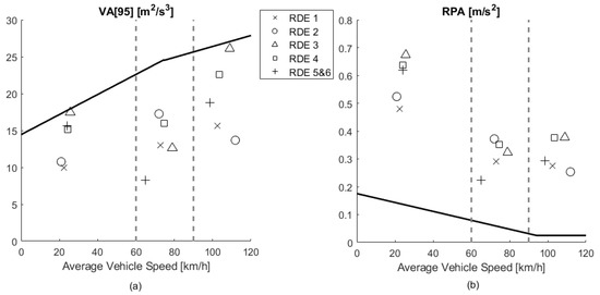
Figure 3.
(a) VA [95] and (b) RPA values in each driving zone for the proposed RDE cycle.
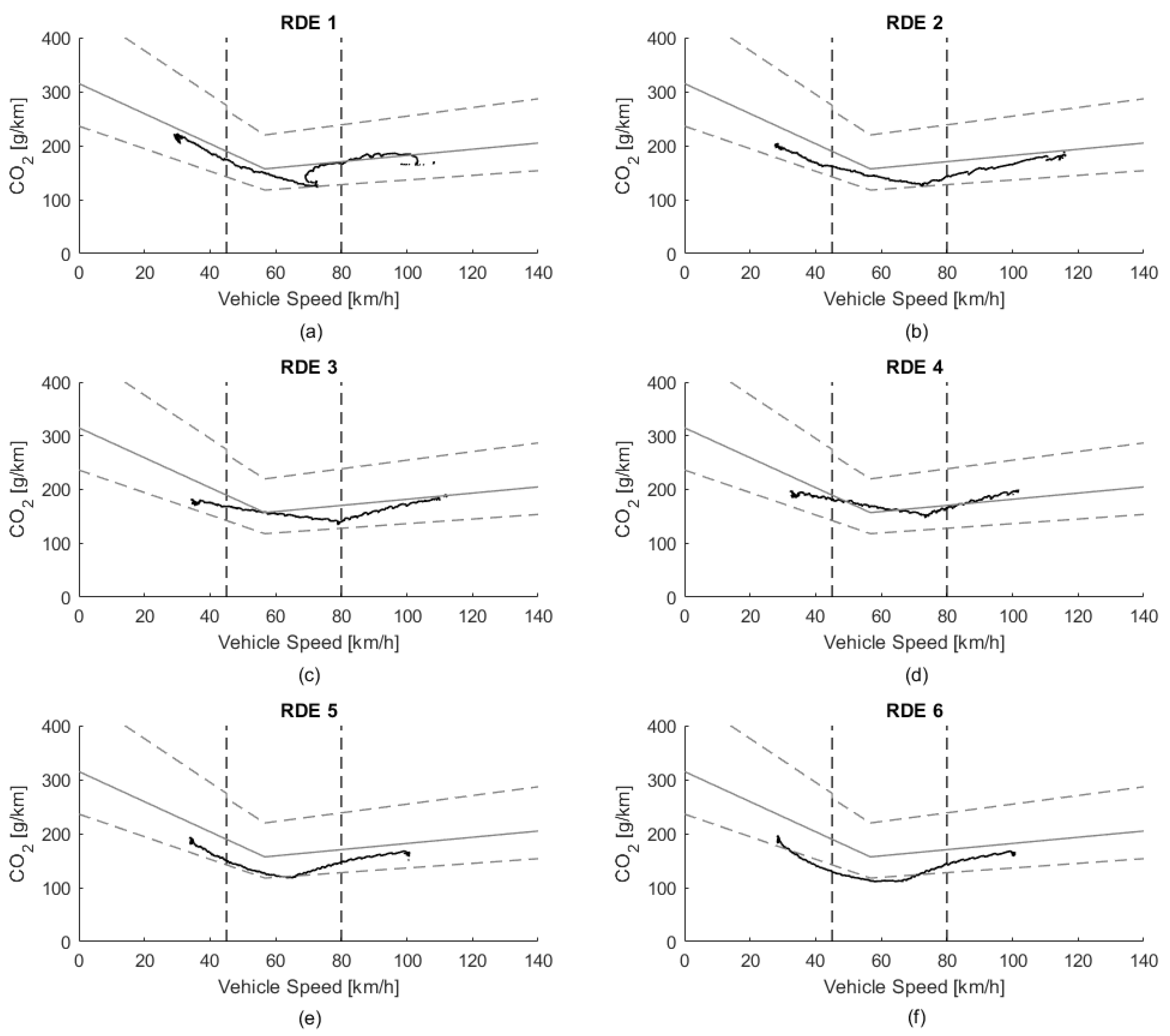
The last calculation corresponds to the Moving Averaging Window (MAW). Such calculation starts from a previously performed WLTC, which serves to obtain the so-called CO2 reference mass, defined as half of the CO2 mass emitted by the vehicle during this WLTC reference test. The CO2 reference mass is used to calculate the MAW as follows: CO2 emissions are cumulated from the beginning of the RDE test (having a sampling frequency of 1 Hz) until reaching the CO2 mass reference. The average speed and the average specific emissions of CO2 in g/km in this period permit the definition of the first window. After resetting the CO2 count to zero, the next window will start a second later and continue with the same calculation method until the end of the cycle. The RDE cycle is only considered valid when at least 50% of urban, rural, and motorway windows are within the tolerances defined by regulation calculated through the CO2 characteristic curve. Figure 4 shows the MAWs of the cycles under study. As observed, all cycles have at least the 50% of MAWs within the tolerances of the CO2 curve for every driving zone. The sixth RDE may seem invalid at first glance because many windows are below the lower limit. Nevertheless, it has 57% within tolerances of the urban zone and 58% of the rural zone, thus complying as well with the requirements of RDE.
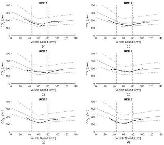
Figure 4.
CO2 curve, tolerances, and MAWs obtained for cycles RDE 1 (a), RDE 2 (b), RDE 3 (c), RDE 4 (d), RDE 5 (e), RDE 6 (f).
4. Results
4.1. RDE Tests
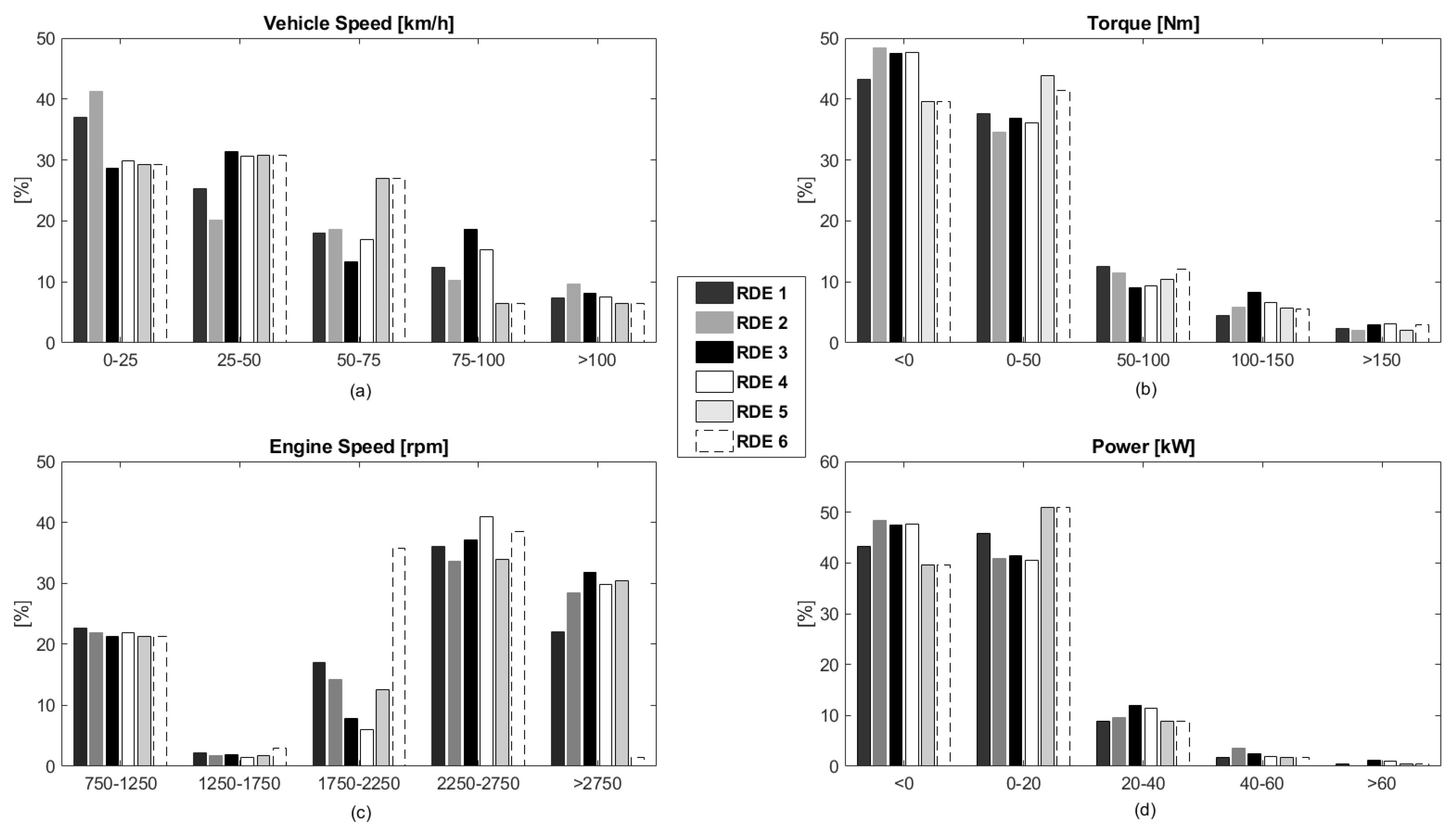
The analysis of cycles was performed by looking at the dynamic variables’ distribution [32]. In this analysis, the vehicle speed, torque, engine speed, and power were divided into five segments. Figure 5 shows the distribution frequency of these parameters for each RDE cycle.

Figure 5.
Distribution of (a) vehicle velocity, (b) torque, (c) engine speed, and (d) power.
In the case of the vehicle speed, the groups were divided into intervals of 25 km/h till up to 100 km/h, and one more for speeds higher than 100 km/h. The engine torque was also divided into groups of 50 Nm. The engine speed was divided into groups of 500 rpm and, finally, the power in groups of 20 kW. The events in which the power and torque were less than zero corresponded to events when the engine was dragging or the driver was braking.
At first sight, the cycles show a great dispersion between each other and consider that all of them are valid, evidencing that a wide variety of cycles fit the regulation. In the case of RDEs 5 and 6, considering that the vehicle speed and power distribution were identical (as defined), the different driver behavior led to different engine operating conditions in terms of torque, engine speed, pedal position, etc. Figure 5c shows that RDE 6 had much fewer points in the strip of greater than 2750 rpm since driver behavior was programmed with the aim that it did before the gearshift, avoiding high engine speed. It could be representative of the down speeding technique [33], which is a current trend where the goal is that the engine works at high performance reducing consumption and, as far as possible, pollutant emissions.
The cycles were divided into 13 different bins depending on vehicle speed and power for a deeper analysis. Table 5 shows the conditions of those bins.
Table 5.
Division of the test into different bins depending on vehicle speed and power.
Figure 6 shows the results of the 13 bins applied to the 6 RDE cycles. It can be seen that the dispersion between these cycles increases in the higher power region (bin 8 onwards). As an example, the RDE 2 cycle does not present any values in bins 8, 11, and 12, which denotes that the power was below 40 kW in the urban area. It can also be observed in RDE 2 bin 13, corresponding to the maximum motorway power fraction, the time proportion was the lowest, corresponding to few accelerations and having steadier driving. Another interesting aspect is that RDE 1 was the only one that went into all bins, which implies that this test would make the engine work in more diverse operating conditions than the other ones.
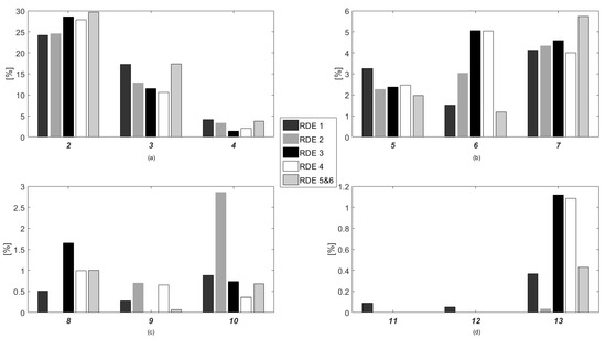
Figure 6.
Bin proportions from 2 to 4 (a), 5 to 7 (b), 8 to 10 (c) and 11 to 13 (d) of each cycle.
Looking at RDEs 3 and 4, and the bins that represent the urban area (3, 6, 9, and 12), the values of bins 3 and 6 are very similar. However, bin 9 of RDE 3 is equal to zero but 0.64% in RDE 4, which involves bigger power that was reached in this cycle in the urban zone due to a higher dynamic solicitation. RPA and VA [95] values also point it out, with RDE 4 above RDE 3, as observed in Figure 3.
Finally, RDEs 5 and 6 are those that have been generated to avoid aggressive driving. It is especially noticeable in the motorway zone, where the highest values are in bin 7 (low power zone), whilst bins 10 and 13 are less representative.
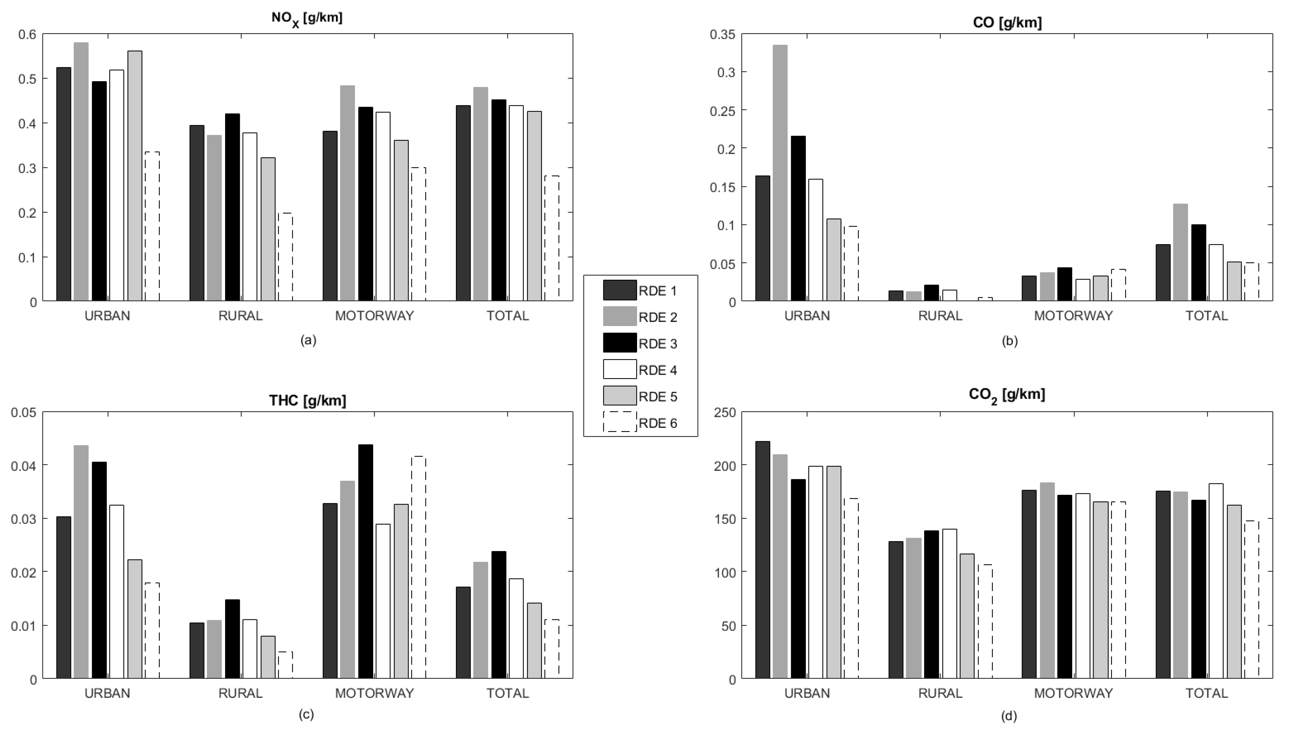
Figure 7 and Table 6 show the specific emissions in grams per kilometer of NOX, CO, THC, and CO2. In case of PM emissions, the particles could not be registered along the entire tests, due to the required purge of the opacimeter. Therefore, global emissions have not been plotted in Figure 7. These specific emissions for three periods of RDE 1 are in Section 4.2 for the sake of completeness. Tests were performed without urea injection so that NOX emissions were above the regulatory limit. On the other hand, THC and CO fulfill the type-approval limits after being oxidized in the DOC.

Figure 7.
NOX (a), CO (b), THC (c) and CO2 (d) pollutant emissions.
Table 6.
RDE pollutants emissions per kilometer.
Figure 7 shows a significant dispersion between pollutant emissions. In the case of NOX emissions, leaving RDE 6 aside (the driver behavior was modified), the differences reached up to 17.39% in an urban zone, 30.88% in the rural zone, and 27.10% in the motorway. The total specific emissions showed the maximum difference of 12.74% between RDEs 2 and 5.
THC and CO strongly depended on the engine and aftertreatment temperatures. RDEs 5 and 6, which were the cycles less loaded, showed the lowest HC emission. These emissions were produced due to incomplete combustion when the engine was yet cold and during phases with high load or high EGR rates where lambda was even below 1. RDE 2 produced the highest CO emissions, which was mainly due to the large contribution in the urban area. This cycle had the lowest urban and total distances, which increased specific emissions per kilometer due to the higher impact of the engine warm-up phase. The other cycles did not show significant differences.
In the case of CO2 emissions, there were also big differences, with RDEs 1 and 2 producing the highest emissions. The biggest difference between RDEs 3 and 4 was the average vehicle speed reduction, which implied an increase in fuel consumption. RDE 5 resulted in the lowest CO2 emission among the cycles with the same driver behavior (RDE 1 to RDE 5).
RDE 1 was the most representative of real driving since it was directly extracted from a cycle performed on road. Comparing RDEs 1 and 2, where the results are similar, contributes to stating that a WLTC presents similar dynamic conditions as an RDE cycle since CO2 and NOX emissions showed analogous values.
The comparison between RDEs 5 and 6 led to characterize the effect of the different driver behavior in the same trip and vehicle speed profile. RDE 6 NOX emissions were reduced by 34% compared to RDE 5. In the case of THC and CO, similar drawdowns were obtained whilst CO2 emissions were decreased by 9.2%.
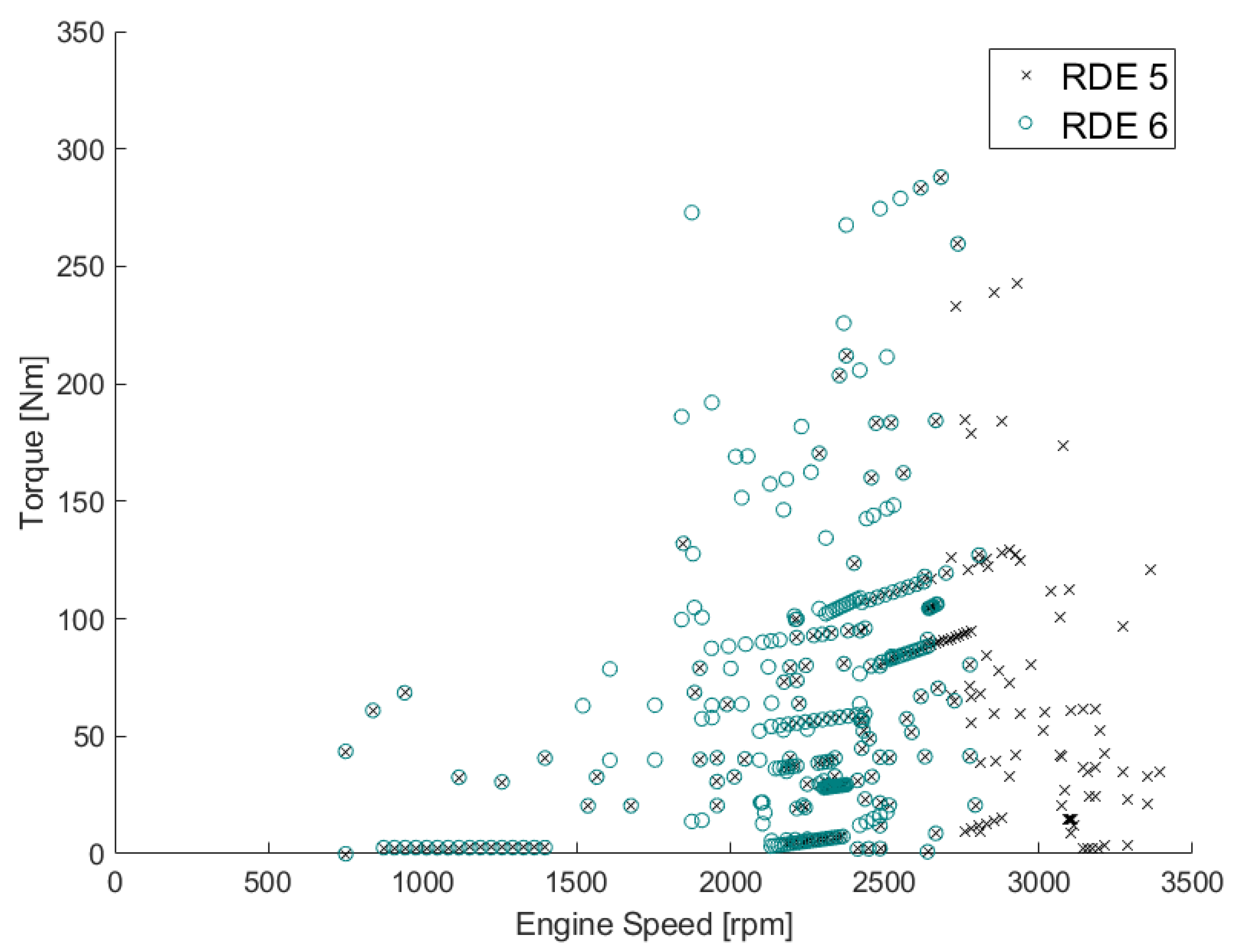
The required engine power to reach a certain vehicle speed in a cycle is obtained from the engine speed and torque. Since the engine speed was reduced in the case of the RDE 6 by varying the shifting procedure, the torque was increased. Figure 8 shows the effective engine torque as a function of engine speed for RDEs 5 and 6. RDE 6 dots are located closer to the top left corner (high torque and low engine speed).
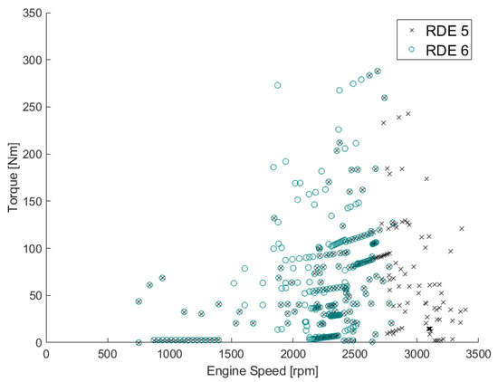
Figure 8.
RDE 5 and RDE 6 engine map comparison.
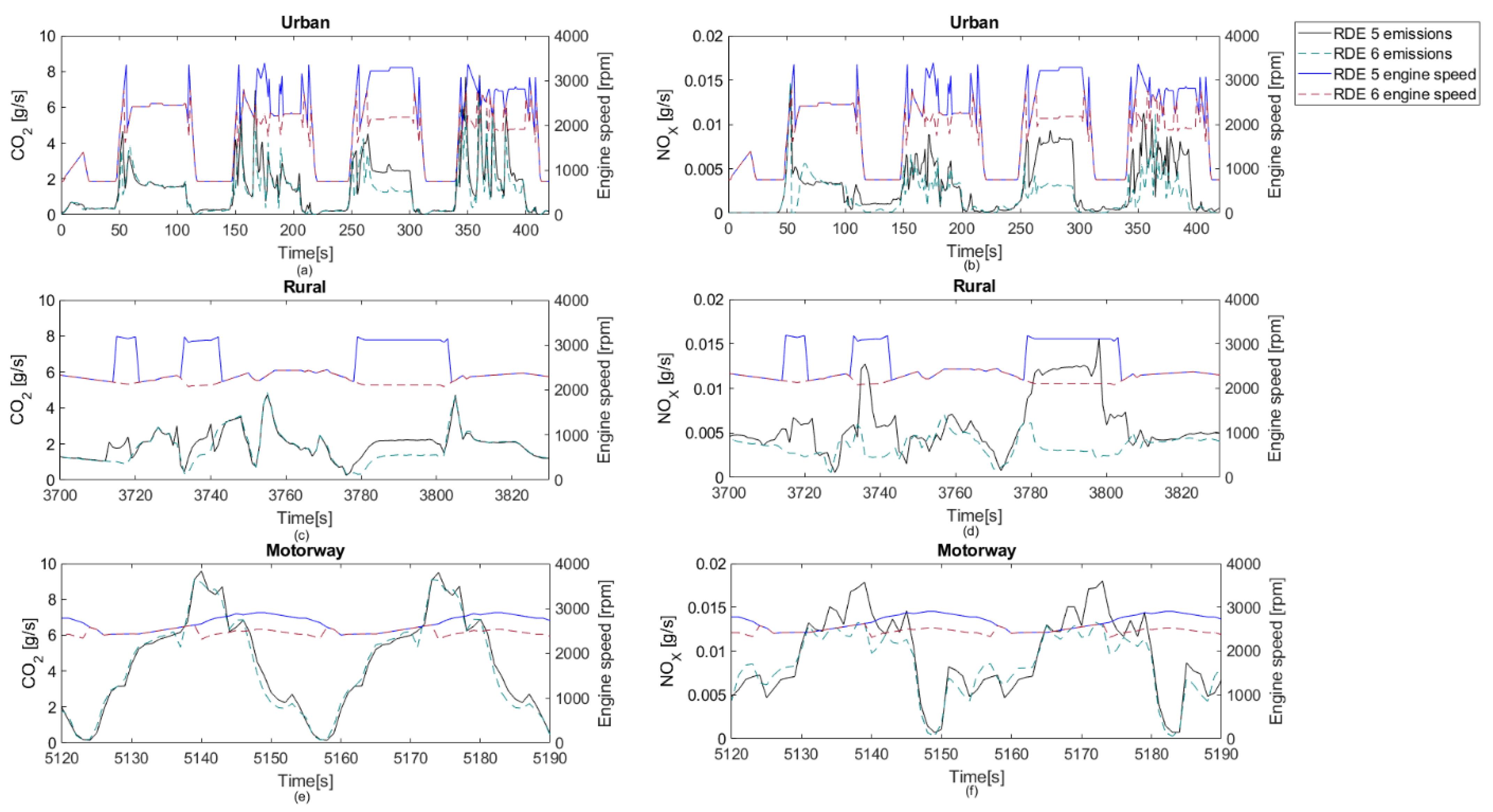
According to the driver behavior, in the case of RDE 5, the engine speed reached higher values while more loaded conditions were characteristic in RDE 6. Figure 9 shows three different fractions of RDE 5 and 6 cycles during urban, rural, and motorway driving, where the differences in CO2 and NOX emissions can be observed.
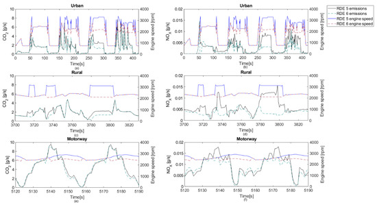
Figure 9.
Comparison of Urban (a), Rural (c) and Motorway (e) CO2 emissions and Urban (b) Rural (d), and Motorway (f) NOX emissions, and engine speed between RDEs 5 and 6.
Figure 9 illustrates emission differences in some specific portions of RDEs 5 and 6 where the engine speed changed. These differences are especially noticed in urban and rural zones, where the engine speed disparity was bigger. In the case of CO2 emissions, benefits were obtained in RDE 6, implying a more efficient driving mode at higher loads. Regarding pollutant emissions, this driving behavior also involved relevant reductions as shown in Figure 7.
4.2. Test Results Versus Map Results
Additionally, an engine mapping study under steady-state conditions was performed to analyze the engine behavior in all possible operating situations. In order to achieve that, the mapping ranged from 1000 rpm to 3500 rpm every 100 rpm, combined with 10% of throttle increments.
The CO2 and NOX emissions are represented in Figure 10. The operating area of RDE 1 is also represented by dots on the contour plots, which are devoted to CO2 and NOX emissions. As observed in Figure 10a, the maximum CO2 emission was located in the top right corner, whilst the minimum was at the bottom left one. However, Figure 10b shows how NOX emissions were mainly influenced by the EGR rate, which is different depending on the operative engine conditions although lower as the load and speed increased.
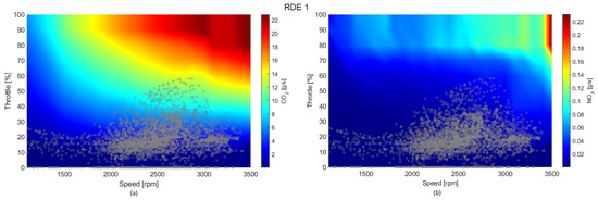
Figure 10.
CO2 [g/s] (a) and NOX [g/s] (b) emission from engine maps (color scale) and those obtained from the tested cycle (dots).
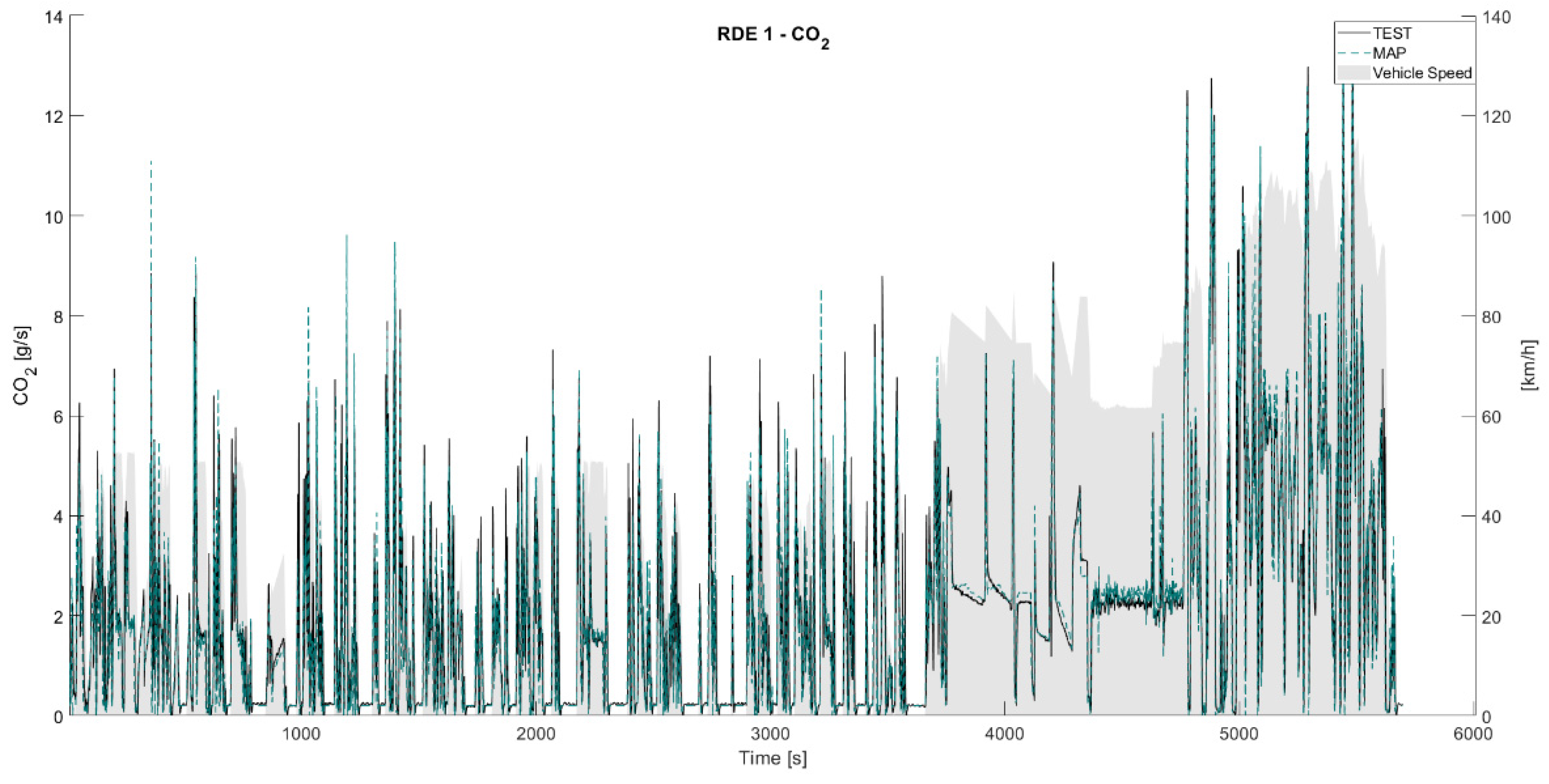
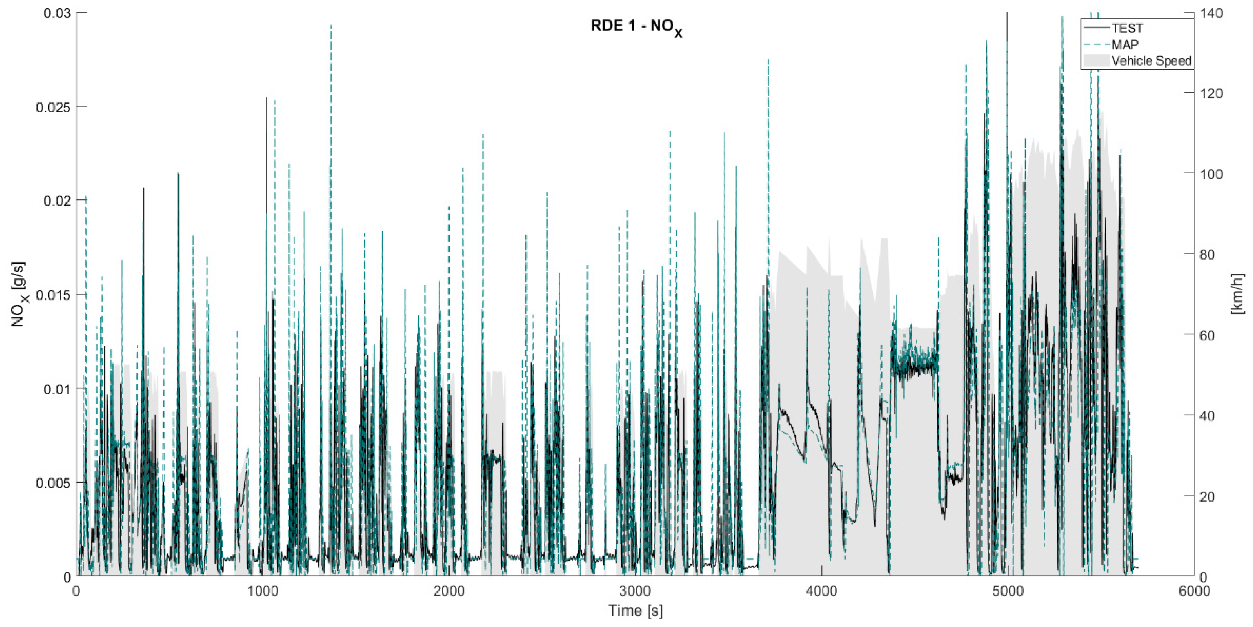
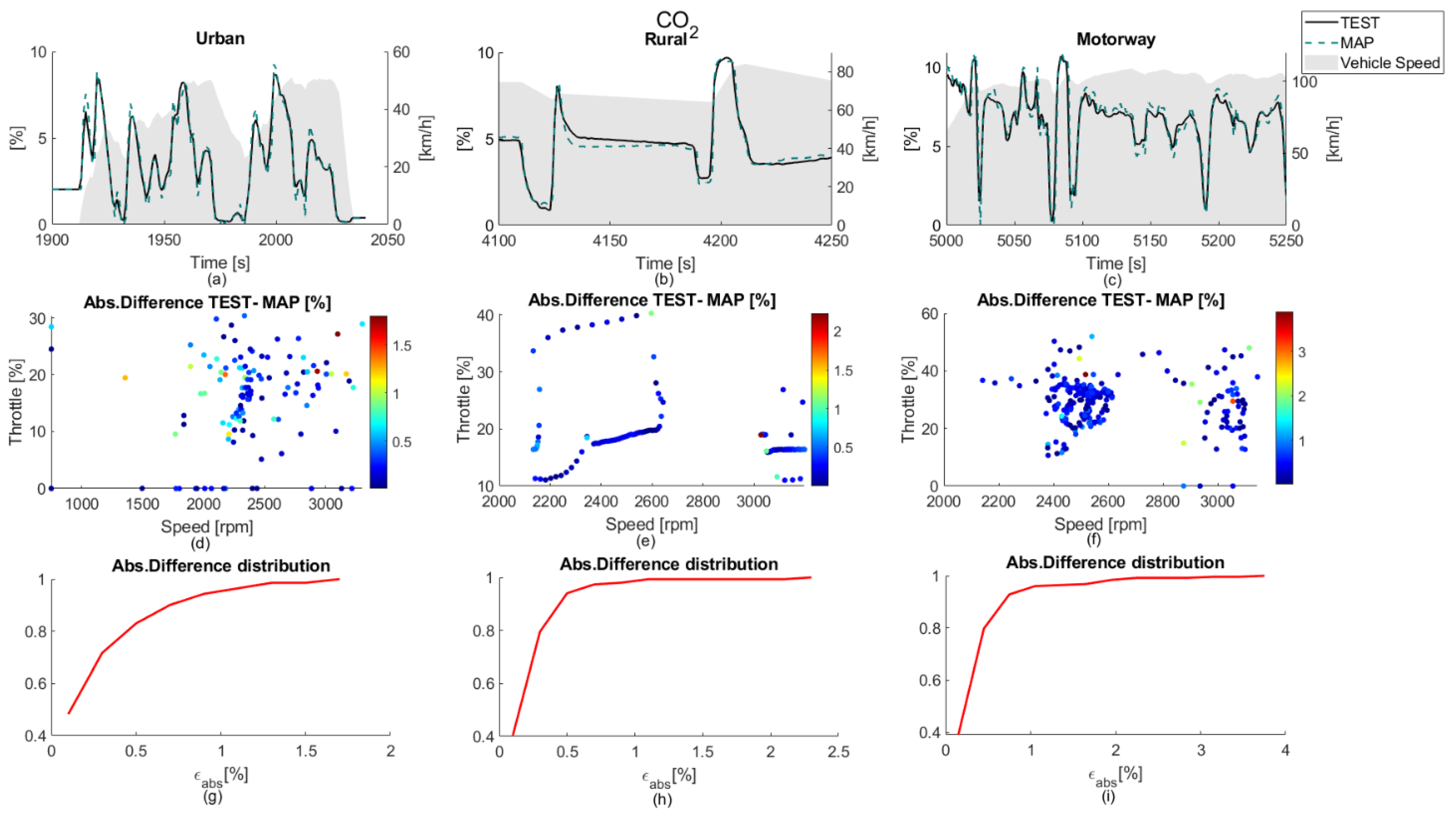
A comparative study of CO2 and NOX emissions obtained from the RDE tests and the steady-state results from the engine map was performed considering the engine speed and throttle during the cycles. Figure 11 and Figure 12 show the instantaneous CO2 and NOX emissions of RDE 1 versus the emissions obtained by interpolation in the engine maps.
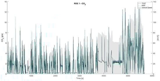
Figure 11.
RDE 1 CO2 [g/s] emissions test versus engine map.

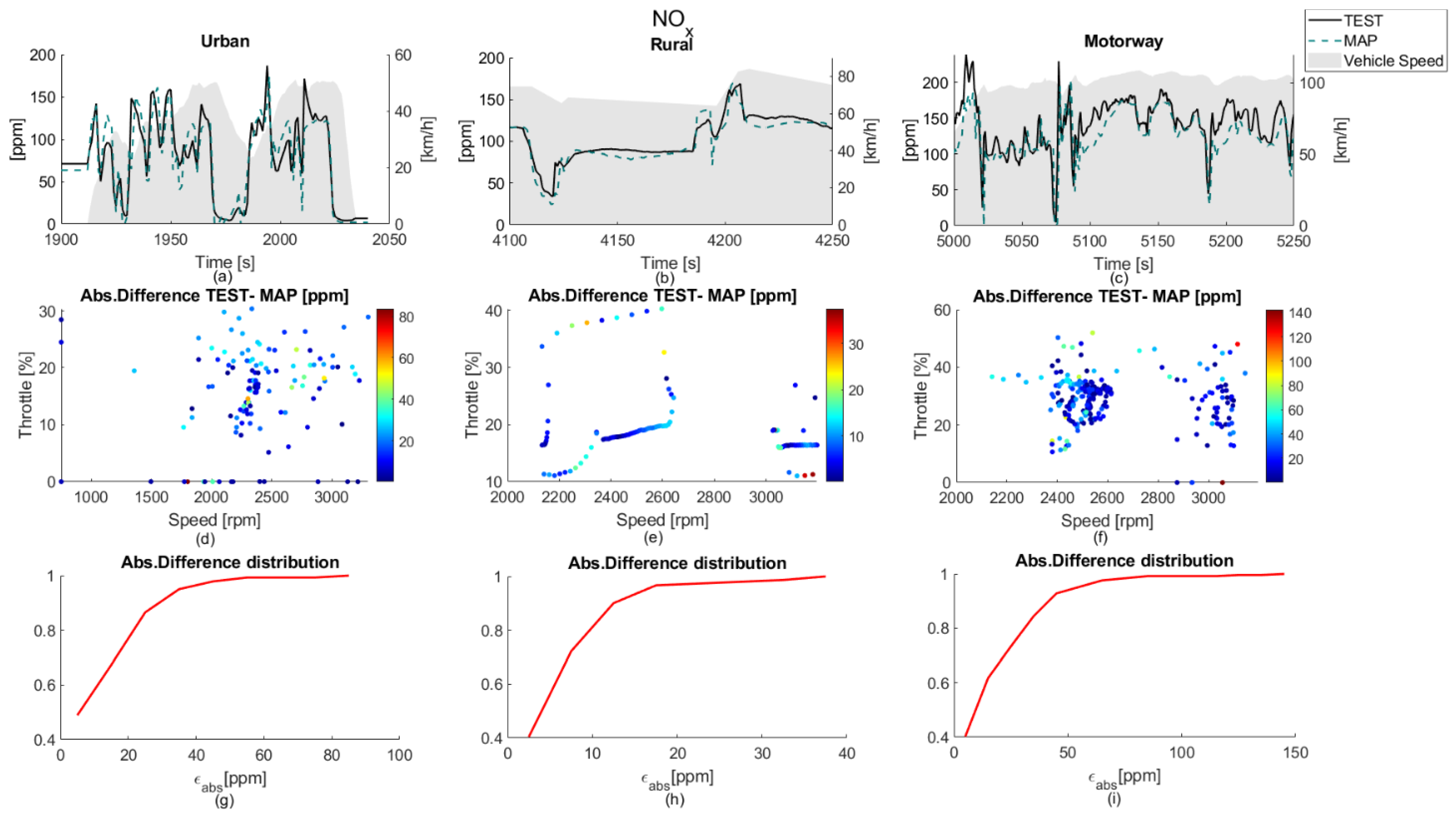
Figure 12.
RDE 1 NOX [g/s] emissions test versus engine map.
As observed in Figure 12, a very good correlation exists between the instantaneous measured values during the tests and the emissions extracted from the maps. The divergencies produced are due to interpolations errors, especially in the case of NOX, since these do not have a total linear behavior.
Making a deeper analysis, Figure 13a–c and Figure 14a–c show three fractions of 150 s of CO2 and NOX emissions in RDE 1 corresponding to urban, rural, and motorway driving phases, respectively. Absolutes differences between emission concentrations in dynamic and steady operation are presented in Figure 13d–f and Figure 14d–f. Finally, Figure 13g–i and Figure 14g–i represent the distribution of the emissions absolute error for these species.
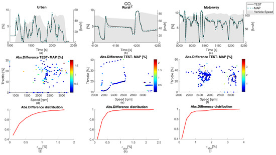
Figure 13.
CO2 emissions comparison between RDE 1 and engine map in urban (a,d,g), rural (b,e,h), and motorway (c,f,i) driving phases.

Figure 14.
NOX emissions comparison between RDE 1 and engine map i urban (a,d,g), rural (b,e,h), and motorway (c,f,i) driving phases.
As can be observed, urban zones show the worst correlation due to their more dynamic feature. However, rural and motorway zones were characterized by quasi-steady operation, where the vehicle speed was almost constant, so that the engine solicitations did not change significantly. In any case, a good correspondence was obtained between RDE and steady-state maps, especially for fuel consumption.
Table 7 shows the comparison of the CO2 and NOX emissions data for all tested RDEs. The corresponding errors are also presented. This summary of the results points out very small differences between pollutants measured during the tests and pollutants extracted from a steady-state engine map. In the case of CO2 emissions, the correlation is better, having errors around 1%, which fell into the measurement error margin of the measuring device. In the case of NOX emissions, the deviation from the engine map estimate increased, but it was still low enough to provide understanding about the driving cycles effects as a function of their definition, especially keeping in mind the use of state-of-the-art NOX aftertreatment systems of high conversion efficiency.
Table 7.
CO2 and NOX pollutants from RDE cycles versus map emissions.
Looking at CO2 errors in Table 7, the largest errors were found in the RDEs 1, 2, 3, and 4 cycles, i.e., the specific emissions were also maximum. On the contrary, RDEs 5 and 6 presented the lowest errors. These results agree with the dynamic solicitations of the cycles since RDEs 5 and 6 were generated to be less aggressive than RDEs 1 to 4. In the case of NOX errors, a clear tendency was not found. In any case, errors were kept below 5% in all cases.
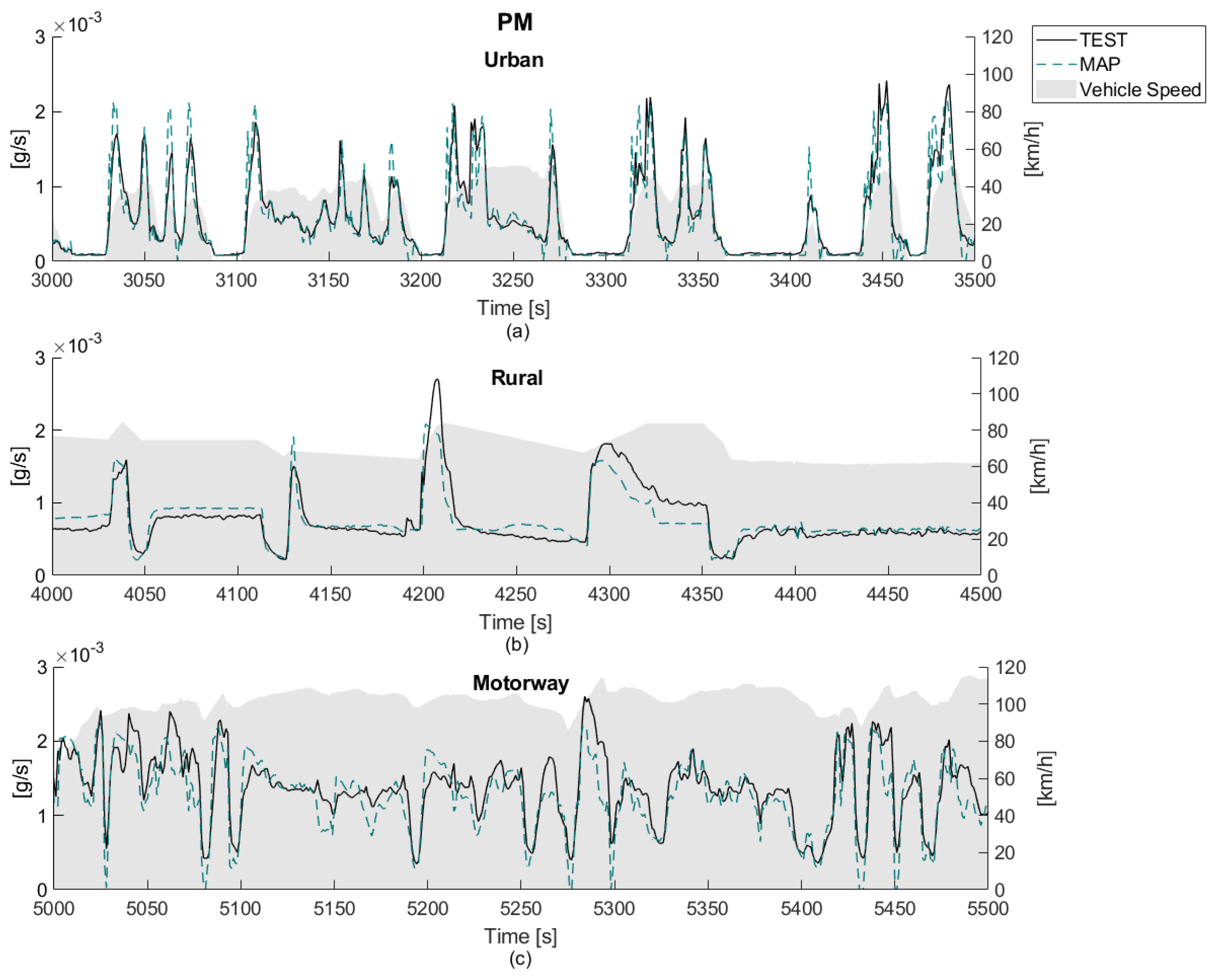
As previously commented, during the tests, it was not possible to measure the PM along the entire driving cycle. However, three different periods of 500 s corresponding to three zones (urban, rural, and motorway) in RDE 1 have been considered. Figure 15 shows RDE PM mass emissions compared to those obtained from the steady-state map.
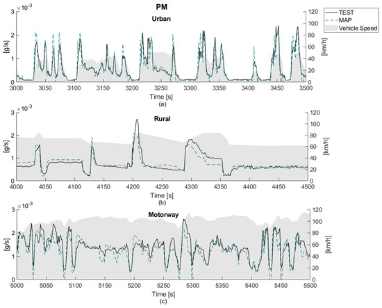
Figure 15.
RDE 1 periods PM urban (a), rural (b) and motorway (c) mass emissions [g/s] test versus engine map.
Figure 15 emissions show a great correlation between emissions measured and emissions from the steady-state map. Table 8 shows the accumulated values of each one of these three phases and the total values represent their summation.
Table 8.
PM mass emissions from RDE 1 versus map emissions.
Looking at PM mass errors, the higher discrepancies appear during the urban and motorway periods, which are characterized by more dynamic conditions due to steeper accelerations. In any case, the interpolation can also be a very helpful tool to estimate the PM in an RDE cycle since the obtained errors are relatively low considering the complexity of this species.
5. Conclusions
In this paper, several RDE cycles with different dynamic characteristics have been performed in an engine test bench. First, an on-road cycle was performed in a vehicle as a baseline; then, a second cycle was defined using transient maneuvers extracted from a WLTP cycle; finally, four additional cycles were defined using a computational tool to generate RDE-compliant conditions from a sub-set of acceleration and deceleration ramps while replicating different driver behavior. This methodology aimed at reducing cost, time, and uncertainties involved in performing a cycle on road, such as climatological conditions, PEMS accuracy, traffic status, and driver behavior. This is particularly relevant for future powertrain systems development since different technologies or calibration strategies can be assessed more reliably and robustly while ensuring RDE representative conditions.
The results showed how RDE cycles with the same driver behavior produced significant emissions dispersion. For instance, variations of 12.74% in the case of NOX and 7.42% in CO2 were found between different cycles. Moreover, a great improvement was seen from an emissions perspective when the gear shift was adjusted to achieve lower engine speed. Particularly, drawdowns in NOX and CO2 emissions of 34% and 9.2%, respectively, have been noted. Instead, CO and THC emissions were mostly linked to the engine and aftertreatment temperature, so the best results are achieved when the engine load is increased.
Finally, an attempt to estimate the cycle emissions from steady-state tests was made. The comparison between such estimation and the actual RDE tests emissions showed a good correlation, within 1.6% accuracy for CO2 and better behavior in less dynamic cycles, 4.6% in the case of NOX, and relatively low errors in the case of PM mass. The deviations observed were due to two phenomena, On the one hand, all emissions during the engine warm-up period differ from the estimations since the engine map was performed with the engine previously warmed up. On the other hand, of NOX and PM mass emissions, and their known trade-off, both showed a non-linear behavior as a function of speed and load, inducing an uncertainty linked to the interpolation inside the steady-state map. This uncertainty could be reduced by performing a more complete engine map, which lowers variations of speed and load between adjacent points but at the cost of higher test bench time. In any case, the analysis performed in this study confirms that steady-state maps can be used to provide a meaningful approximation of these emissions during a realistic certification cycle.
Author Contributions
J.M.L.: methodology, conceptualization, writing—original draft, supervision; P.P.: validation, writing—review and editing; J.d.l.M.: formal analysis, writing—review and editing; F.R.: investigation, data curation, visualization, writing—original draft. All authors have read and agreed to the published version of the manuscript.
Funding
This research has been supported by Grant PID2020-114289RB-I00 funded by MCIN/AEI/10.13039/501100011033.
Conflicts of Interest
The authors declare no conflict of interest.
References
- Council Directive 91/441/EEC of 26 June 1991 Amending Directive 70/220/EEC on the Approximation of the Laws of the Member States Relating to Measures to Be Taken against Air Pollution by Emissions from Motor Vehicles. Available online: http://data.europa.eu/eli/dir/1991/441/oj (accessed on 1 December 2021).
- Commission Regulation (EC) No 692/2008 of 18 July 2008 Implementing and Amending Regulation (EC) No 715/2007 of the European Parliament and of the Council on Type-Approval of Motor Vehicles with Respect to Emissions from Light Passenger and Commercial Vehicles (Euro 5 and Euro 6) and on Access to Vehicle Repair and Maintenance Information. Available online: http://data.europa.eu/eli/reg/2008/692/oj (accessed on 1 December 2021).
- State of the Global Climate in 2020, Provisional Report; World Meteorological Organization (WMO): Geneva, Switzerland, 2020.
- Center for Climate and Energy Solutions. Outcomes of the UN climate change conference in Paris. In Proceedings of the 21st Session of the Conference of the Parties to the United Nations Framework Convention on Climate Change (COP 21), Paris, France, 30 November–12 December 2015. [Google Scholar]
- Pandey, D.; Agrawal, M.; Pandey, J.S. Carbon footprint: Current methods of estimation. Environ. Monit. Assess 2011, 178, 135–160. [Google Scholar] [CrossRef] [PubMed]
- IEA. Energy Technology Perspectives; Technical Report; International Energy Agency: Paris, France, 2014; Available online: https://www.iea.org/reports/energy-technology-perspectives2014 (accessed on 10 December 2021).
- Regulation (EC). No 443/2009 of the European Parliament and of the Council of 23 April 2009 Setting Emission Performance Standards for New Passenger Cars as Part of the Community’s Integrated Approach to Reduce CO2 Emissions from Light-Duty Vehicles. J. Eur. Union 2009, 140, 5–6. [Google Scholar]
- Regulation (EU). 2019/631 of the European Parliament and of the Council of 17 April 2019 Setting CO2 Emission Performance Standards for New Passenger Cars and for New Light Commercial Vehicles, and Repealing Regulations (EC) No 443/2009 and (EU) No 510/2011; European Union: Brussels, Belgium, 2019. [Google Scholar]
- Zhang, L.; Lin, J.; Qiu, R. Characterizing the toxic gaseous emissions of gasoline and diesel vehicles based on a real-world on-road investigation. J. Clean. Prod. 2021, 286, 124957. [Google Scholar] [CrossRef]
- Tutuianu, M.; Bonnel, P.; Ciuffo, B.; Haniu, T.; Ichikawa, N.; Marotta, A.; Pavlovic, J.; Steven, H. Development of the World-wide harmonized Light duty Test Cycle (WLTC) and a possible pathway for its introduction in the European legislation. Transp. Res. Part D Transp. Environ. 2015, 40, 61–75. [Google Scholar] [CrossRef]
- Commission Regulation (EU) 2016/427 of 10 March 2016 amending Regulation (EC) No 692/2008 as Regards Emissions from Light Passenger and Commercial Vehicles (Euro 6). Available online: https://eur-lex.europa.eu/legal-content/EN/TXT/PDF/?uri=CELEX:32016R0427&from=ES (accessed on 1 December 2021).
- Lee, H.; Lee, K. Comparative Evaluation of the Effect of Vehicle Parameters on Fuel Consumption under NEDC and WLTP. Energies 2020, 13, 4245. [Google Scholar] [CrossRef]
- Dimaratos, A.; Toumasatos, Z.; Doulgeris, S.; Triantafyllopoulos, G.; Kontses, A.; Samaras, Z. Assessment of CO2 and NOx Emissions of One Diesel and One Bi-Fuel Gasoline/CNG Euro 6 Vehicles during Real-World Driving and Laboratory Testing. Front. Mech. Eng. 2019, 5. [Google Scholar] [CrossRef] [Green Version]
- Luján, J.M.; Bermúdez, V.; Dolz, V.; Monsalve-Serrano, J. An assessment of the real-world driving gaseous emissions from a Euro 6 light-duty diesel vehicle using a portable emissions measurement system (PEMS). Atmos. Environ. 2018, 174, 112–121. [Google Scholar] [CrossRef]
- García-Contreras, R.; Soriano, J.A.; Fernández-Yáñez, P.; Sánchez-Rodríguez, L.; Mata, C.; Gómez, A.; Armas, O.; Cárdenas, M.D. Dolores Cárdenas, Impact of regulated pollutant emissions of Euro 6d-Temp light-duty diesel vehicles under real driving conditions. J. Clean. Prod. 2021, 286, 124927. [Google Scholar] [CrossRef]
- Commission Regulation (EU) 2018/1832 of 5 November 2018 Amending Directive 2007/46/EC of the European Parliament and of the Council, Commission Regulation (EC) No 692/2008 and Commission Regulation (EU) 2017/1151 for the Purpose of Improving the Emission Type Approval Tests and Procedures for Light Passenger and Commercial Vehicles, Including Those for In-Service Conformity and Real-Driving Emissions and Introducing Devices for Monitoring the Consumption of Fuel and Electric Energy. Available online: https://eur-lex.europa.eu/legal-content/EN/TXT/HTML/?uri=CELEX:32018R1832&from=EN (accessed on 14 December 2021).
- Zhang, L.; Hu, X.; Qiu, R.; Lin, J. Comparison of real-world emissions of LDGVs of different vehicle emission standards on both mountainous and level roads in China. Transp. Res. Part D Transp. Environ. 2019, 69, 24–39. [Google Scholar] [CrossRef]
- Faria, M.V.; Duarte, G.O.; Varella, R.A.; Farias, T.L.; Baptista, P.C. How do road grade, road type and driving aggressiveness impact vehicle fuel consumption? Assessing potential fuel savings in Lisbon, Portugal. Transp. Res. Part D Transp. Environ. 2019, 72, 148–161. [Google Scholar] [CrossRef]
- Bodisco, T.; Zare, A. Practicalities and Driving Dynamics of a Real Driving Emissions (RDE) Euro 6 Regulation Homologation Test. Energies 2019, 12, 2306. [Google Scholar] [CrossRef] [Green Version]
- Triantafyllopoulos, G.; Katsaounis, D.; Karamitros, D.; Ntziachristos, L.; Samaras, Z. Experimental assessment of the potential to decrease diesel NOx emissions beyond minimum requirements for Euro 6 Real Drive Emissions (RDE) compliance. Sci. Total Environment. 2017, 618, 2306. [Google Scholar] [CrossRef] [PubMed]
- Yang, Z.; Liu, Y.; Wu, L.; Martinet, S.; Zhang, Y.; Andre, M.; Mao, H. Real-world gaseous emission characteristics of Euro 6b light-duty gasoline- and diesel-fueled vehicles. Transp. Res. Part D Transp. Environ. 2020, 78, 102215. [Google Scholar] [CrossRef]
- Taborda, A.M.; Varella, R.A.; Farias, T.L.; Duarte, G.O. Evaluation of technological solutions for compliance of environmental legislation in light-duty passenger: A numerical and experimental approach. Transp. Res. Part D Transp. Environ. 2019, 70, 135–146. [Google Scholar] [CrossRef]
- Luján, J.M.; Bermudez, V.; Pla, B.; Redondo, F. Engine test bench feasibility for the study and research of real driving cycles: Pollutant emissions uncertainty characterization. Int. J. Engine Res. 2021. [Google Scholar] [CrossRef]
- Broatch, A.; Margot, X.; Gil, A.; Galindo, E.; Soler, R. Definition of wind blowers for vehicles testing at chassis-dyno facilities using a CFD approach. Transp. Res. Part D Transp. Environ. 2017, 55, 99–112. [Google Scholar] [CrossRef]
- Rodríguez-Fernández, J.; Hernández, J.J.; Ramos, Á.; Calle-Asensio, A. Fuel economy, NOx emissions and lean NOx trap efficiency: Lessons from current driving cycles. Int. J. Engine Res. 2021. [Google Scholar] [CrossRef]
- Claßen, J.; Krysmon, S.; Dorscheidt, F.; Sterlepper, S.; Pischinger, S. Real Driving Emission Calibration—Review of Current Validation Methods against the Background of Future Emission Legislation. Appl. Sci. 2021, 11, 5429. [Google Scholar] [CrossRef]
- Giechaskiel, B.; Casadei, S.; Mazzini, M.; Sammarco, M.; Montabone, G.; Tonelli, R.; Deana, M.; Costi, G.; Di Tanno, F.; Prati, M.V.; et al. Inter-Laboratory Correlation Exercise with Portable Emissions Measurement Systems (PEMS) on Chassis Dynamometers. Appl. Sci. 2018, 8, 2275. [Google Scholar] [CrossRef] [Green Version]
- Varella, R.A.; Giechaskiel, B.; Sousa, L.; Duarte, G. Comparison of Portable Emissions Measurement Systems (PEMS) with Laboratory Grade Equipment. Appl. Sci. 2018, 8, 1633. [Google Scholar] [CrossRef] [Green Version]
- Czerwinski, J.; Comte, P.; Zimmerli, Y.; Reutimann, F. Testing emissions of passenger cars in laboratory and on-road (PEMS, RDE). Combust. Engines 2016, 166, 17–23. [Google Scholar] [CrossRef]
- Daniel, C.N. Estudio de las Emisiones de Escape en Motores de Combustión Interna Alternativos Utilizando Diferentes Sistemas de Control de Contaminantes; Departamento de Máquinas y Motores Térmicos, Universidad Politecnica de Valencia: Valencia, Spain, 2016. [Google Scholar]
- Robert Bosch GmbH. Bosch Automotive Handbook, 10th ed.; John Wiley & Sons: West Sussex, UK, 2018. [Google Scholar]
- Chong, H.S.; Park, Y.; Kwon, S.; Hong, Y. Analysis of real driving gaseous emissions from light-duty diesel vehicles. Transp. Res. Part D Transp. Environ. 2018, 65, 485–499. [Google Scholar] [CrossRef]
- Kogo, T.; Hamamura, Y.; Nakatani, K.; Toda, T.; Kawaguchi, A.; Shoji, A. High efficiency diesel engine with low heat loss combustion concept—Toyota’s inline 4-cylinder 2.8-liter ESTEC 1GD-FTV engine; SAE Paper; SAE: Warrendale, PA, USA, 2016. [Google Scholar] [CrossRef]


Publisher’s Note: MDPI stays neutral with regard to jurisdictional claims in published maps and institutional affiliations. |
© 2022 by the authors. Licensee MDPI, Basel, Switzerland. This article is an open access article distributed under the terms and conditions of the Creative Commons Attribution (CC BY) license (https://creativecommons.org/licenses/by/4.0/).