Modeling Open Channel Flows of a Viscous Fluid: Critical Transition and Apparent Bottom

Abstract

The Shallow Water model (SWM) provides a simplification of the Navier–Stokes model (NSM) for stratified flows over a topography when the depth of the fluid layer is small compared to the horizontal scale of the flow. Nevertheless, the application of SWM is limited to the case of slowly variable bottoms and fails in describing the fluid flow over steep obstacles. In this work, we propose to extend the applicability of SWM when the topography is no longer slowly variable with space, by replacing the topography with an “apparent bottom”. This methodology is tested for the laminar flow of a two-layer fluid over a semi-circular cylinder. Sixteen different steady configurations are investigated in order to assess the influence of the Froude number and the blocking factor corresponding to the ratio between the obstacle height and the fluid layer normal height. Here, the apparent bottom required for SWM is obtained by enforcing the liquid height profile to be the one obtained from full resolution (NSM).

1. Introduction

The Shallow Water model (SWM) is largely used to describe the dynamics of stratified flows such as air and water in open channel flows, lakes and oceans, or atmospheric flows, where the air is decomposed into several layers [1,2]. The SWM is derived from the Navier–Stokes model (NSM) in the limit of small fluid layer depth compared to the horizontal scale of the flow. Thus, the approximation is valid only when the boundary layer is slowly variable. The SWM fails to describe the flow over abrupt obstacles, which we will call “macro-rugosities” in contrast to wall rugosities that can be modeled by “wall-laws”.

Examples of turbulent flow over macro-rugosities include atmospheric boundary layer over an urban canopy or mountain, which often leads to Lee waves generation [3,4,5,6]. The flows of lava [7], ice-sheets [8] or debris avalanches [9], instead, are examples of environmental flows in the laminar regime. The simplest model describing these kind of flows is the one derived in [10].

The problem of a two-layer flow over an abrupt topography has been studied in [11,12,13,14,15,16], where the “topography” is normally represented by a semi-circular cylinder. The free surface inviscid flow over this geometry has been subjected to a large number of theoretical studies, such as [17,18].

The fluid and semi-cylindrical obstacle interaction takes a variety of forms, depending on the normal (upstream) Froude number

$$F_n=\frac{U_n}{\sqrt{g{h}_{n}cos\theta }}$$

(1)

and the blocking factor

$$\alpha =\frac{H}{h_n}$$

(2)

where H is the maximum obstacle height, $h_n$ is the initial undisturbed layer depth, $U_n$ is the velocity of the initial undisturbed fluid layer and $\theta$ is the bottom slope.

Assuming non-viscous flow and horizontal bottom, a theoretical curve for the trans-critical transition has been derived in [4,19] and is given by

$$\alpha =1-\frac{3}{2}{F}_n^{2/3}+\frac{1}{2}{F}_n^2.$$

(3)

This solution is shown in Figure 1 (solid lines). Under the lower branch, the flow is sub-critical in the entire domain while it remains super-critical above the upper branch. In the interval delimited by the two branches, different configurations of trans-critical flow can be observed.

The phase diagram shown in Figure 1 had been first derived numerically in [4] and successively verified through experiments in other works, e.g., [20], for high Reynolds Number flows. Many different regimes have been found experimentally for two-layer flows [20,21,22,23,24,25], three-layer flows [19], or flows with a continuous density gradient [26].

The two-layer turbulent flow over a semi-cylindrical obstacle has been also studied numerically using the Volume of Fluid Method (VOF) and the standard $k-ϵ$ turbulent model in [27,28,29], the CLEAR-VOF method and a large eddy simulation (LES) in [30], and an interface-tracking algorithm for computation of the free-surface with a moving grid in [31].

Most of the works on stratified flows consist of investigating the evolution of a free-surface when the bottom is known a priori. However, in many problems that are currently of interest, the position and the fluid velocity on the free-surface are given, but the shape and location of the solid bottom are unknown a priori. These free-surface problems are called indirect problems. The indirect problem can be solved using minimization techniques which are able to predict all the different shapes and positions of the bottom and solve iteratively the system with the boundary integral method. This is the basis of the minimal high method [32,33], the extremal pressure method [34,35], the extremal energy method [36], and the minimal kinetic energy method [37].

Inverse problems have been extensively investigated, since it is not always possible to retrieve the correct parameters for the predictions. Methods used in the literature include an approach to estimate the open boundary conditions subject to tidal waves [38], stochastic approach based on the measure theory [39], estimation of the bottom topography using a simplified one-dimensional barotropic model [40], Dual Integral Porosity model [41], Variational Data Assimilation [42], lubrication type model for generalized Newtonian fluids equation combined with the Variational Data Assimilation formulation [43], 1D hydraulic models [44], Proper Orthogonal Decomposition [45] and depth specific electrical conductivity [46].

In this work, we present a novel methodology to resolve the inverse problem via a “multi-scale” approach. In particular, we use the results of NSM to infer the parameters of the SWM. We introduce a fictitious surface: the “apparent-bottom” (AB), which is the bottom that corresponds to a given position of the free-surface in the SWM. This methodology shows how a steep topography should be transformed, in order to obtain reliable predictions of a stratified flow with the SWM.

The free-surface data have been generated from the simulation of two-layer flows, obeying the NSM, for different blocking factors and Froude numbers. It is also suggested that the “apparent bottom”, i.e., the transformed steep topography, is a function of the local velocity variance $\beta$ and the local friction factor $\lambda$. For a slowly variable topography, these parameters are approximately constant, and the results of the SWM and NSM are comparable, whereas in the case of a steep topography, neglecting the change of these parameters limits the predicting power of SWM.

In Section 2, both NSM and SWM are presented and both the profile shape factor $\beta$ and dissipation parameter $\lambda$ are defined. The configuration, the boundary conditions and the numerical scheme for the simulations are presented in Section 3. The systematic comparison of the steady states of both NSM and SWM is performed in Section 4 for the sixteen values of the couple $(F_n,\alpha )$. An analysis of both $\beta \left(x\right)$ and $\lambda \left(x\right)$ is performed in Section 5, followed by the computation of the apparent bottom for the sixteen cases.

2. The Navier–Stokes and the Shallow Water Models

2.1. Navier–Stokes Model (NSM)

A stratified flow of a heavy and light fluid with densities ${\rho }_1$ and ${\rho }_2$, respectively, is modeled with the NSM. The VOF Method, introduced in [47], is used to describe the stratified flow in this study. The volume fraction $\gamma \in [0,1]$ is thus used to track the free surface of the heavier fluid such that $\gamma =1$ is the heavier fluid and $\gamma =0$ is the lighter fluid, the average density being defined by

$$\rho ={\rho }_1\gamma +{\rho }_2\left(1-\gamma \right).$$

(4)

We consider a two-dimensional domain and the equations are solved in the $\left(x,z\right)$ coordinate system, whose axis z is perpendicular to the bottom wall outside the obstacle and is rotated clock-wise by an angle $\theta$ with respect to the gravitational axis. The bottom is defined by the equation $z=Z\left(x\right)$ where $Z\left(x\right)=0$ everywhere except at the semi-cylindrical obstacle of radius H.

The volume averaged velocity field, whose components are u and w, obey the mass conservation equation

$$\frac{\partial u}{\partial x}+\frac{\partial w}{\partial z}=0$$

(5)

and the momentum equations read

$$\rho \left(\frac{\partial u}{\partial t}+u\frac{\partial u}{\partial x}+w\frac{\partial u}{\partial z}\right)=-\frac{\partial p}{\partial x}+\rho gsin\theta +2\sigma \kappa {\widehat{n}}_x+\frac{\partial }{\partial x}\left[2\mu \frac{\partial u}{\partial x}\right]+\frac{\partial }{\partial z}\left[\mu \left(\frac{\partial u}{\partial z}+\frac{\partial w}{\partial x}\right)\right]$$

(6)

$$\rho \left(\frac{\partial w}{\partial t}+u\frac{\partial w}{\partial x}+w\frac{\partial w}{\partial z}\right)=-\frac{\partial p}{\partial z}-\rho gcos\theta +2\sigma \kappa {\widehat{n}}_z+\frac{\partial }{\partial x}\left[\mu \left(\frac{\partial u}{\partial z}+\frac{\partial w}{\partial x}\right)\right]+\frac{\partial }{\partial z}\left[2\mu \frac{\partial w}{\partial z}\right]$$

(7)

where p is the pressure, g is the gravitational acceleration, $\sigma$ is the surface tension and $\mu$ is the dynamic viscosity of the mixture defined by

$$\mu ={\mu }_1\gamma +{\mu }_2\left(1-\gamma \right).$$

(8)

The evolution of the volume fraction $\gamma$, according to [47], is given by the following transport equation

$$\frac{\partial \gamma }{\partial t}+u\frac{\partial \gamma }{\partial x}+w\frac{\partial \gamma }{\partial z}=0.$$

(9)

The free surface S of the heavier fluid can be defined as:

$$S=\left\{(x,z)\in \Omega :\gamma (t,x,z)-0.5=0\right\}$$

(10)

whose normal is defined as

$$\widehat{n}=\nabla \gamma$$

(11)

and the curvature

$$\kappa =-\frac{1}{2}\left(\frac{\partial n_x}{\partial x}+\frac{\partial n_z}{\partial z}\right).$$

(12)

Surface tension $\sigma$ is included in the numerical simulations to regularize the interface but the sensitivity of the results presented here is negligible with respect to this force. We assume that S is sufficiently smooth to be described by the equation $z=Z_s(t,x)$.

2.2. Shallow Water Model (SWM)

When ${\rho }_1$ is large compared to ${\rho }_2$, which we assume here, the vertical integration of the Navier–Stokes equations over the heavy layer leads to the Shallow Water equations. We define the heavier fluid depth h and the mean longitudinal velocity U as:

$$h(t,x)=Z_s(t,x)-Z\left(x\right)$$

(13)

and

$$U(t,x)=\frac{1}{h(t,x)}{\int }_{Z\left(x\right)}^{Z_s(t,x)}u(t,x,z)dz.$$

(14)

The pressure is assumed to be hydrostatic,

$$p(t,x,z)=p_2+{\rho }_{1}gcos\theta \left(Z_s(t,x)-z\right)$$

(15)

and $p_2$, the pressure of the lighter fluid, is constant. Integrating Equations (5)–(7) on the vertical axis z and taking into account the surface boundary conditions, we obtain the SWM

$$\frac{\partial h}{\partial t}+\frac{\partial }{\partial x}\left(Uh\right)=0,$$

(16)

$$\frac{\partial }{\partial t}\left(Uh\right)+\frac{\partial }{\partial x}\left(\beta U^{2}h+gcos\theta \frac{h^2}{2}\right)=-ghcos\theta \frac{\partial Z}{\partial x}+ghsin\theta -3\nu \lambda \frac{U}{h},$$

(17)

where $\nu ={\mu }_1/{\rho }_1$ is the kinematic viscosity, $\beta$, which measures the variance of the velocity profile, is defined by:

$$\beta (t,x)=\frac{1}{U^2(t,x)h(t,x)}{\int }_{Z\left(x\right)}^{Z_s(t,x)}{u}^2(t,x,z)dz,$$

(18)

and $\lambda$, which measures this momentum dissipation, is defined by:

$$\lambda (t,x)=-\frac{1}{3}\frac{h}{U}{\int }_{Z\left(x\right)}^{Z_s(t,x)}\left[\frac{{\partial }^{2}u}{\partial x^2}(t,x,z)+\frac{{\partial }^{2}u}{\partial z^2}(t,x,z)\right]dz.$$

(19)

In the case of a laminar flow on a flat bottom, one obtains $\beta =1.2$ and $\lambda =1$. The departure from these values can be due to the adjustment of the flow to a non vanishing topography $Z\left(x\right)$.

For a given mass flux q, we, respectively, denote $h_n$ and $U_n$, the height and the mean velocity of the normal flow defined by the relations

$$\left\{\begin{array}{c}{\displaystyle q=h_n{U}_n}\hfill \\ {\displaystyle 0=g{h}_{n}sin\theta -3\nu \frac{U_n}{h_n}.}\hfill \end{array}\right.$$

(20)

This solution corresponds to the steady flow on an infinite inclined plane, characterized by a balance between gravitational acceleration and viscous dissipation.

The local Froude number $F(t,x)$ is defined by

$$F=\frac{U}{\sqrt{ghcos\theta }}.$$

(21)

When $\beta (t,x)$ and $\lambda (t,x)$ are prescribed, the Shallow Water Equations (16) and (17) are hyperbolic and the two wave velocities read

$$V_{\pm }=\beta U\left(\frac{1+\beta }{2}\pm \sqrt{\frac{1-\beta }{2}+\frac{1}{F^2}}\right).$$

(22)

Steady solutions are such that $h\left(x\right)$, $U\left(x\right)$$\beta \left(x\right)$ and $\lambda \left(x\right)$ satisfy the ordinary differential equation

$$\left(1-\beta F^2\right)\frac{dh}{dx}=tan\theta -\frac{dZ}{dx}-F^2\left(\frac{d\beta }{dx}+\frac{3\nu \lambda }{q}\right)\mathrm{with}q=hU\mathrm{constant}.$$

(23)

The critical condition is thus obtained for $F={\beta }^{-1/2}$ for both wave propagation and backwater curves. In the present SW simulations both the $\beta$ and $\lambda$ parameters are considered constant and equal to 1. Since the flow under investigation is laminar, it can be argued that this choice for the $\beta$ parameter is incorrect. Nevertheless, this is due to the fact that a $\beta \ne 1$ will allow the SW to be Galilean invariant.

3. Numerical Simulations of a Laminar Flow over an Obstacle

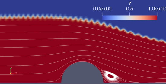
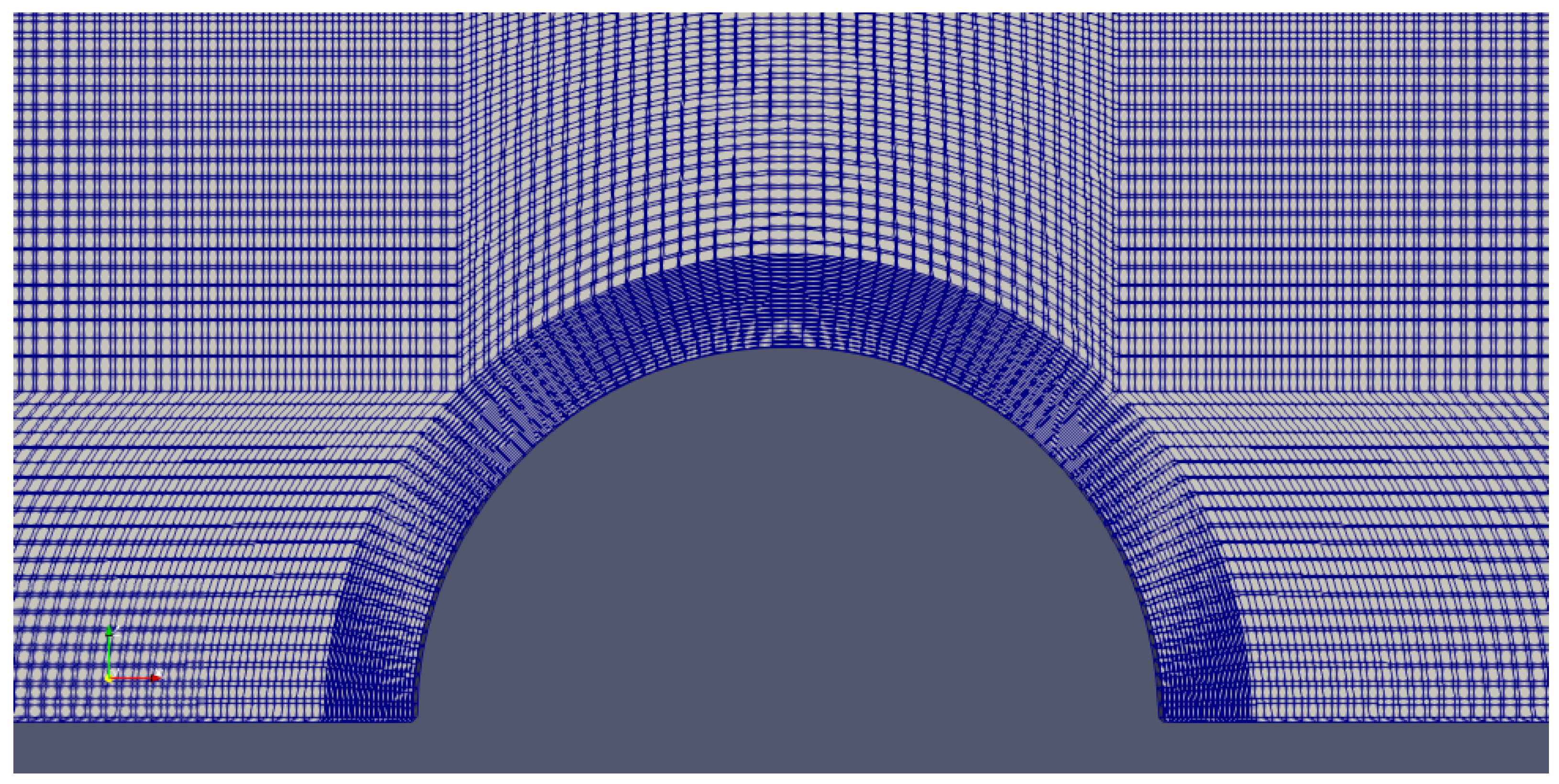
3.1. Configuration with a Half Cylinder

We consider a topography $Z\left(x\right)$ describing a bump in the form of a semicircular cross-section whose axis is orthogonal to the mean flow. The radius of the section is denoted by H.

We consider the following control parameters: the normal Froude number $F_n$, the blocking factor $\alpha$, the slope angle $\theta$ and the normal Reynolds number

$$R_n=\frac{q}{\nu }.$$

(24)

The equilibrium (20) implies $R_{n}tan\theta =3F_n^2$. We define a “geometrical Reynolds number” $R_g$ through the relation

$$R_g=\frac{\sqrt{gH}H}{\nu }=3F_n{\alpha }^{1.5}{(cos\theta )}^{-1/2}{(sin\theta )}^{-1}.$$

(25)

This parameter would be constant in a real experiment where both $\theta$ and q could be varied with g (gravity), H (obstacle) and $\nu$ (fluid) being fixed quantities. In this study, we fix $R_g=26$ and explore the sixteen cases obtained by choosing $\alpha \in \{0.8,0.6,0.4,0.2\}$ and $F_n\in \{0.25,0.75,1.25,1.75\}$. The relations (20) and (25) with $R_g=26$ provide the values of $R_n$ and $\theta$ as functions of $F_n$ and $\alpha$, as computed in

Table 1. Normal Reynolds numbers $R_n$ and bottom slope angles $\theta$ in degrees as function of the Froude number $F_n$ and blocking factor $\alpha$ for the chosen value $R_g=26$ of the geometrical Reynolds number.

$({\mathit{R}}_{\mathit{n}},\mathit{\theta })$	$\mathit{\alpha }=0.8$	$\mathit{\alpha }=0.6$	$\mathit{\alpha }=0.4$	$\mathit{\alpha }=0.2$
$F_n=0.25$	(9, 1.18${}^{\circ }$)	(14, 0.77${}^{\circ }$)	(26, 0.42${}^{\circ }$)	(73, 0.15${}^{\circ }$)
$F_n=0.75$	(27, 3.54${}^{\circ }$)	(42, 2.30${}^{\circ }$)	(77, 1.25${}^{\circ }$)	(218, 0.44${}^{\circ }$)
$F_n=1.25$	(45, 5.89${}^{\circ }$)	(70, 3.83${}^{\circ }$)	(128, 2.09${}^{\circ }$)	(363, 0.74${}^{\circ }$)
$F_n=1.75$	(63, 8.22${}^{\circ }$)	(98, 5.36${}^{\circ }$)	(180, 2.92${}^{\circ }$)	(509, 1.03${}^{\circ }$)

. For these cases, the maximum value of $R_n$, obtained for $F=1.75$ and $\alpha =0.2$, is of the order of 500. Thus, the flow can be considered as laminar for these numerical experiments.

For the following simulations, we have imposed ${\rho }_1=1000$ kg·m${}^{-3}$, ${\mu }_1=1$ Pa·s for the heavier fluid and ${\rho }_2=1$ kg·m${}^{-3}$${\mu }_2=14.8$ Pa·s for the lighter fluid in order to have the same density and viscosity ratios as those of water and air. The domain considered is 50 times larger than the obstacle height H and 12 times higher. The details of the computational grid are shown in Figure 2.

3.2. Boundary Conditions

Only two boundary conditions are required for the SWM, since it is made up of two first order partial differential equations. At the inlet, we impose the flow rate $q=U(t,x_{in})h(t,x_{in})$. We suppose that the inlet height $h_n=h(t,x_{in})$ is given by Equation (17) when the local Froude number is smaller than 1, but is fixed to its actual value when $F_n\ge 1$ (critical regime with no return to the fluvial regime). At the outlet, we impose a zero-gradient condition when the local Froude number is smaller than 1, but we let h obey Equation (16) when $F_{out}\ge 1$.

Imposing boundary conditions for the NSM is more complex. We again suppose that the inlet height $h_n=h(t,x_{in})$ is given by Equation (17) when the local Froude number is smaller than 1, but is fixed to its actual value when $F_n\ge 1$. For the velocity, we impose the inlet boundary conditions

$$u(t,x_{in},z)=\left\{\begin{array}{cc}{\displaystyle u_{in}\left(z\right)=\frac{3q}{2h_n}\frac{z}{h_n}\left(2-\frac{z}{h_n}\right)}\hfill & \mathrm{if}z\le h_n,\hfill \\ {\displaystyle u_{in}\left(z\right)=u_{in}\left(h_n\right)=\frac{3q}{2h_n}}\hfill & \mathrm{if}z>h_n,\hfill \end{array}\right.\mathrm{and}w(t,x_{in},z)=0.$$

(26)

At the outlet, we impose an advective boundary condition for the velocity field, which is equivalent to implicitly assuming an equilibrium between the friction and hydrostatic pressure. Zero-gradient conditions are assumed for the volume fraction at every boundary.

3.3. Numerical Scheme

In this paper, the VOF system is solved with the OpenFOAM CFD Toolbox, which is widely used in the CFD Community [48,49]. The interFoam solver, available for the two-phase VOF calculations, has been modified in order to incorporate the desired Froude-dependent boundary conditions. The developed code allows to solve Equations (5)–(9) via the PISO algorithm.

For the simulation of the SWM, we use a CENTRAL UPWIND discretization scheme for hyperbolic problems as given in [50,51]. The fourth order Runge-Kutta method (RK4) is used to advance the solution in time. The method has been implemented in a FORTRAN, used in the CFD community [52], code and the fields are initialized from the OpenFOAM results.

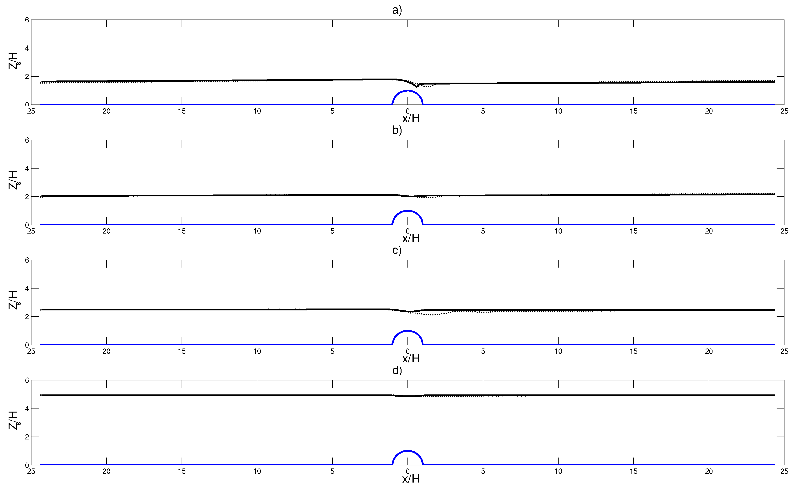
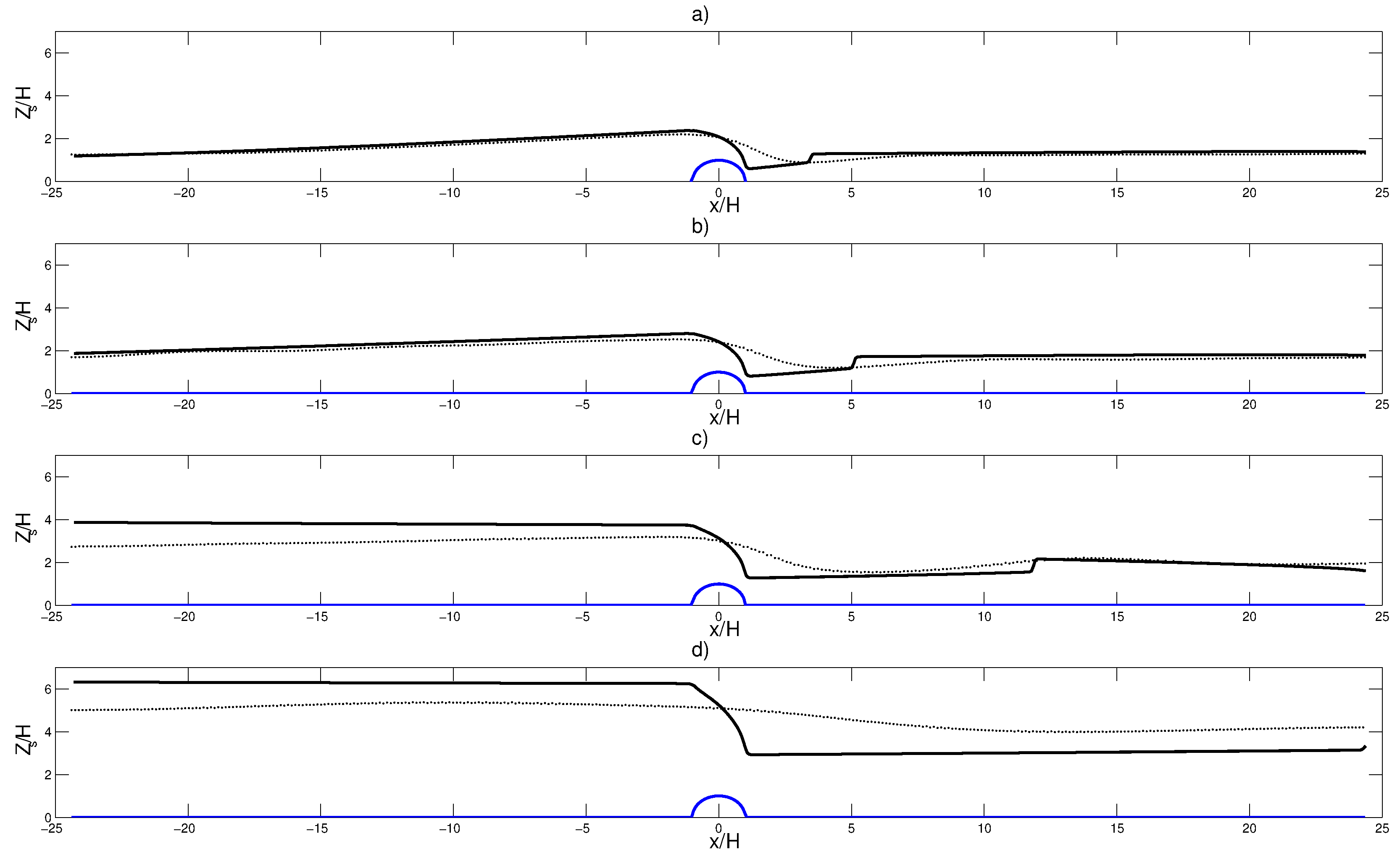
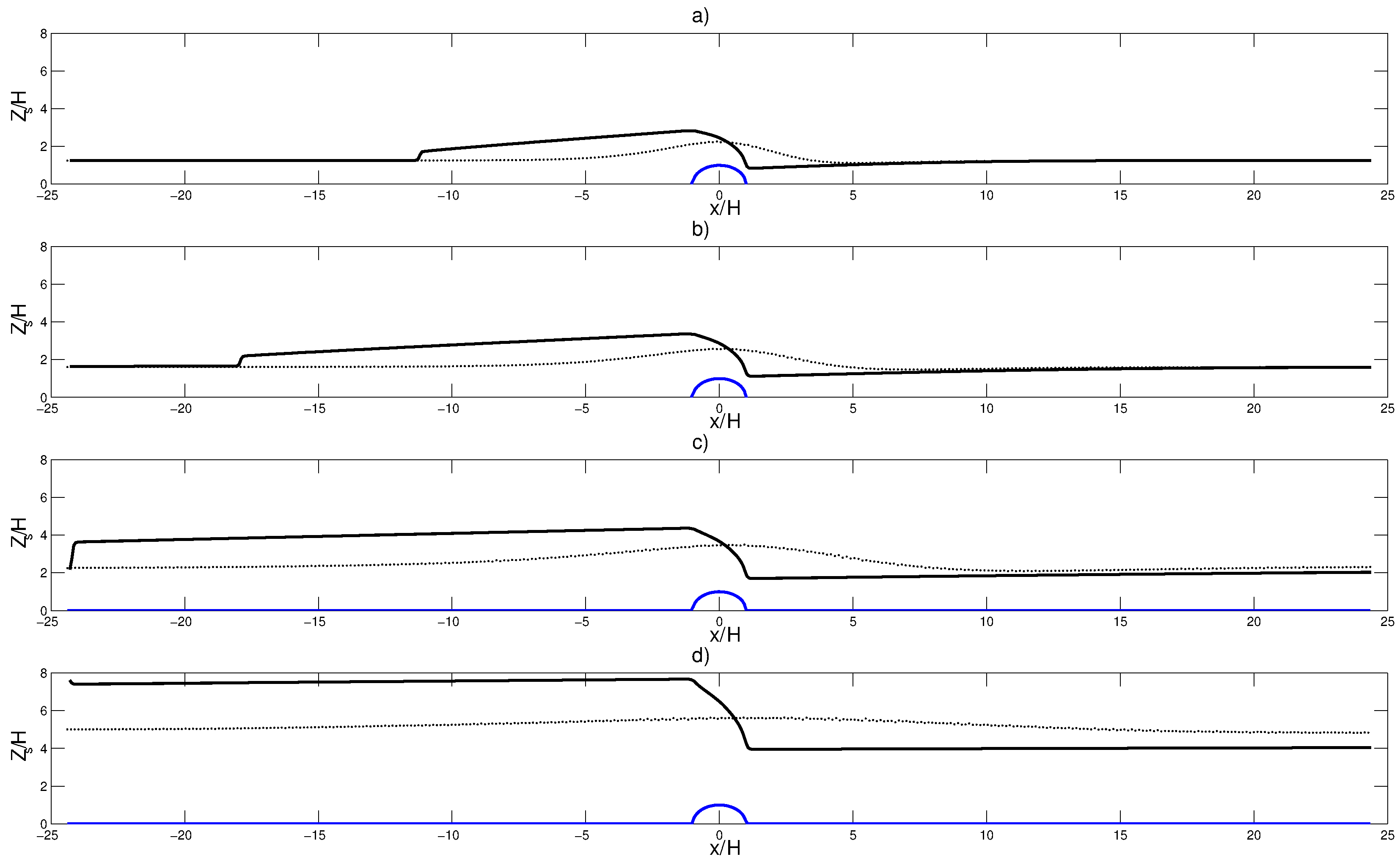
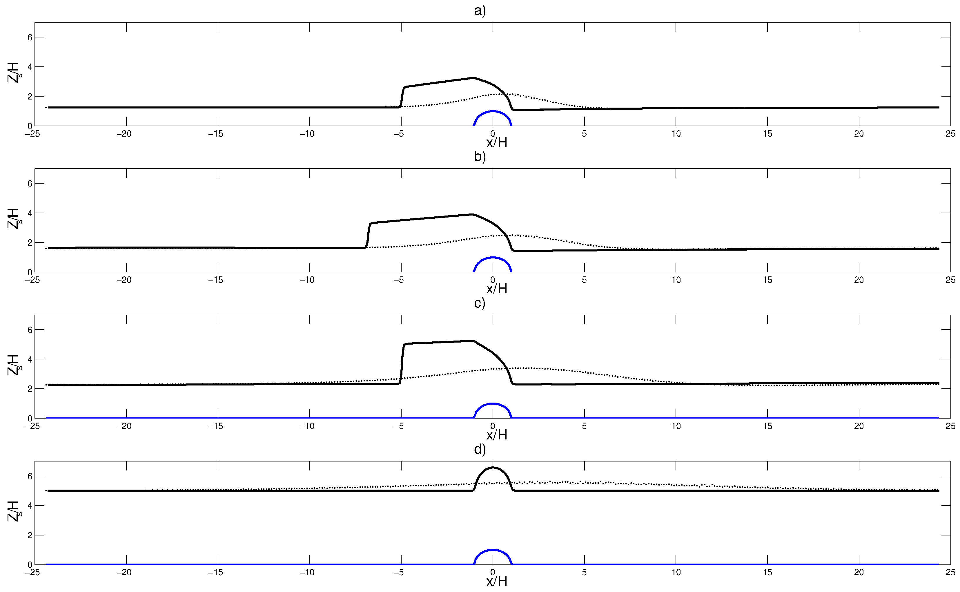
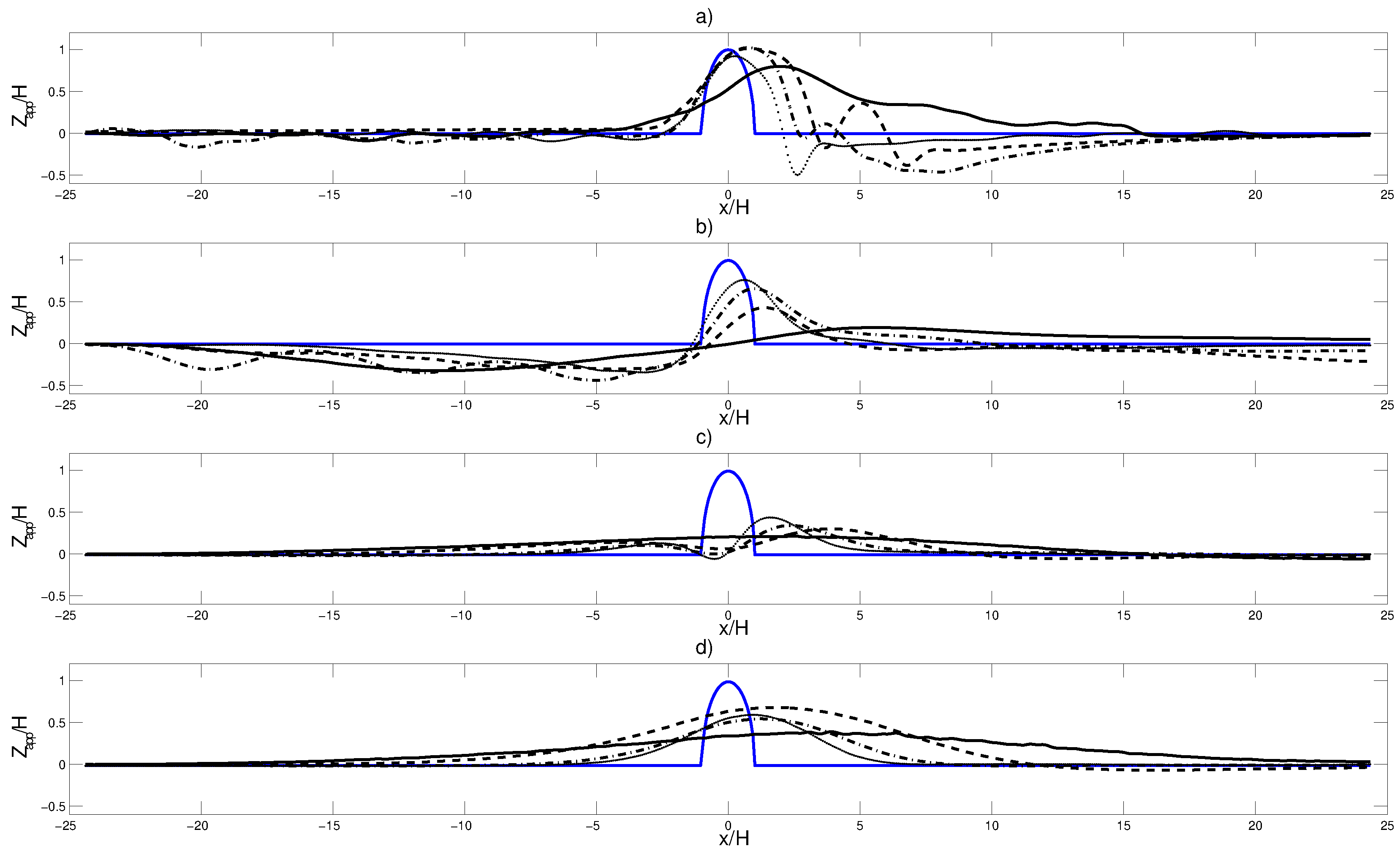
4. Comparison of Surface Heights between NSM and SWM

In this section, we compare the steady solutions of the NSM with those of the SWM. The comparison is made in terms of the free surface height $Z_s$. In each figure, we present the results at different equilibrium Froude number $F_n$, which plays the most important part in the determination of the flow regime. Every figure is divided into four sub-figures which shows the influence of the blocking factor $\alpha$ at a given $F_n$.

4.1. Case $F_n=0.25$

The heavier fluid level profiles of the steady solutions of both NSM and SWM for the case $F_n=0.25$ are displayed in Figure 2. These are the cases in which there is the best match between the two models. The presence of the obstacle causes a local diminution of pressure which is compensated by the acceleration of the fluid. The fluid acceleration causes a contraction of the free-surface as well. The slope is low and the depth h is almost constant, so the free surface is mostly parallel to the bottom except near the obstacle.

The results of both models are in good agreement for $\alpha =0.4$ and $\alpha =0.2$. The main differences between the two models consist of the position and amplitude of the minimum depth. The NSM predicts that the minimum is not located at the top of the obstacle, but is shifted downstream and lowered. From the SWM point of view this is as if the NSM would “see” the obstacle move from its original position. Besides this, on the heavier liquid surface, there are secondary oscillations which are completely damped out at a distance of almost 5 heights from the obstacle center. These are the Stokes-waves seen in [53,54,55,56], but in our case, since we deal with a highly viscous fluid, they are muffled at a short distance from their source.

4.2. Case $F_n=0.75$

In Figure 3, the results for the depth $h\left(x\right)$ calculated at $F_n=0.75$ are presented. In this case, a downstream hydraulic jump can be observed in the SW results. Its distance from the obstacle increases with decreasing $\alpha$. For $\alpha =0.2$ (Figure 4d), the hydraulic jump is not visible, because the domain is not long enough. It must be remembered that the comparison is made on equal $F_n$ and different $\alpha$ but not on equal Reynolds number $R_n$, which influences the dissipation and, therefore, the position of the hydraulic jump. In the NSM, the hydraulic jump is clearly smoothed over the stream-wise direction, probably due to a local viscous dissipation which is not accounted for in the SWM.

It must be noted that the depth in the SWM is higher than the one in NSM. This is because, during the transient period, a bore propagates downstream the obstacle. This phenomenon has been observed in [4,57]. The bore height depends on the flow rate, or, at a given Froude number, on the parameter $\alpha$. Comparing the results of the NSM with the SWM, we can see that the agreement is higher for low values of the blocking factor. In general, the profile predicted by the NSM is smoother as compared to the SWM.

4.3. Case $F_n=1.25$

In Figure 5, the case of $F_n=1.25$ is analyzed. In this case, we still have a hydraulic jump in the SWM. The difference from the previous case is that, here, the hydraulic jump is located upstream the obstacle. For this case the SWM gives a typical trans-critical curve, with a sub-critical flow upstream the obstacle and a super-critical flow downstream. In the transient period, a bore is departed from the obstacle upstream, but in this case, at a certain distance from the weir, which grows with decreasing $\alpha$, the bore stops as observed in [4,57]. In Figure 5d, this is not visible because the domain is probably not long enough and the bore can get out. The results of the NSM are very different. In fact, for all the blocking factors, the $Z_s$ profile has the typical shape of the super-critical case, and no jump is observed. The free-surface follows the bottom profile and, approaching the obstacle, it rises rather than falling, while moving away from the obstacle it falls instead of rising unlike in the sub-critical case.

4.4. Case $F_n=1.75$

The last case analyzed here is $F_n=1.75$. The results shown in Figure 5a–c are not much different from those obtained for $F_n=1.25$ but the distance between the bore and the obstacle, in the SWM, is smaller and the height of the bore, higher. This is due to the fact that, for a given flow rate, the higher the Froude number upstream a hydraulic jump, the lower it is downstream. At the obstacle, the motion becomes trans-critical and downstream the equilibrium depth is reached earlier. During the transient simulation, a bore departing from the obstacle travels upstream and stops at a certain distance from it.

The last case, depicted in Figure 5d is different, the motion is completely super-critical and no hydraulic jump is observed. The free-surface $Z_s$ is parallel to the bottom upstream and downstream and follows the obstacle shape showing the maximum height at the top of the obstacle. This is in agreement with the theoretical critical curve displayed in Figure 1, in which we can see that for $F_n=1.75$ and $\alpha =0.2$ there are no hydraulic jumps. The NS model results are similar to those obtained for $F_n=1.25$ in terms of $Z_s$ at least. The free-surface profile has the typical super-critical shape, but looking at Figure 6d, we realize that the results deviate significantly from the SWM.

The free-surface predicted in the NSM, is much lower and wider as compared to the SWM. It looks like the NSM “sees” the obstacle wider and lower than what it actually is. The maximum of $Z_s$ does not correspond to the maximum of the obstacle. This was true in the previous case as well, but here it is more evident.

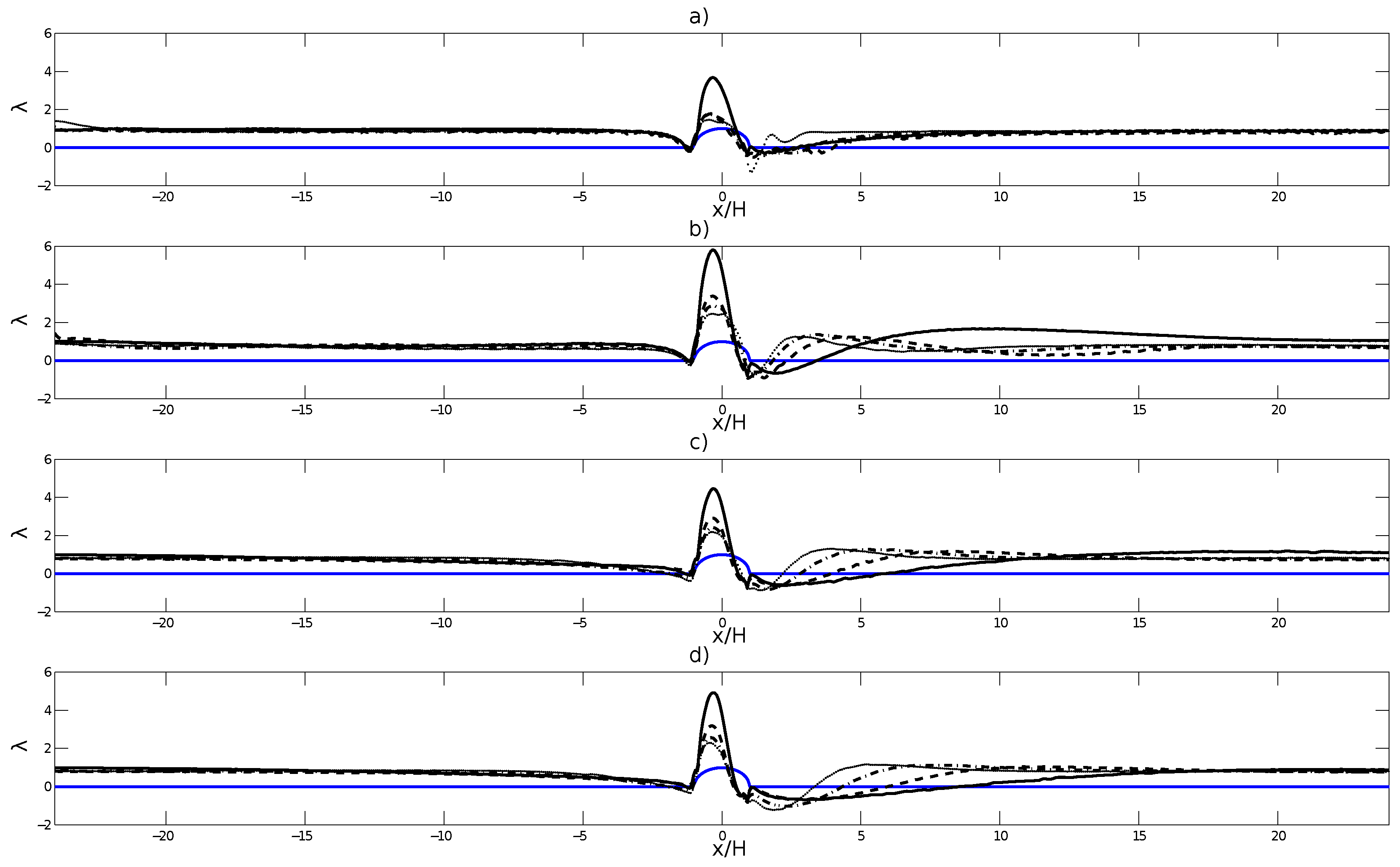
5. Enhanced Parametrization for the SW Model

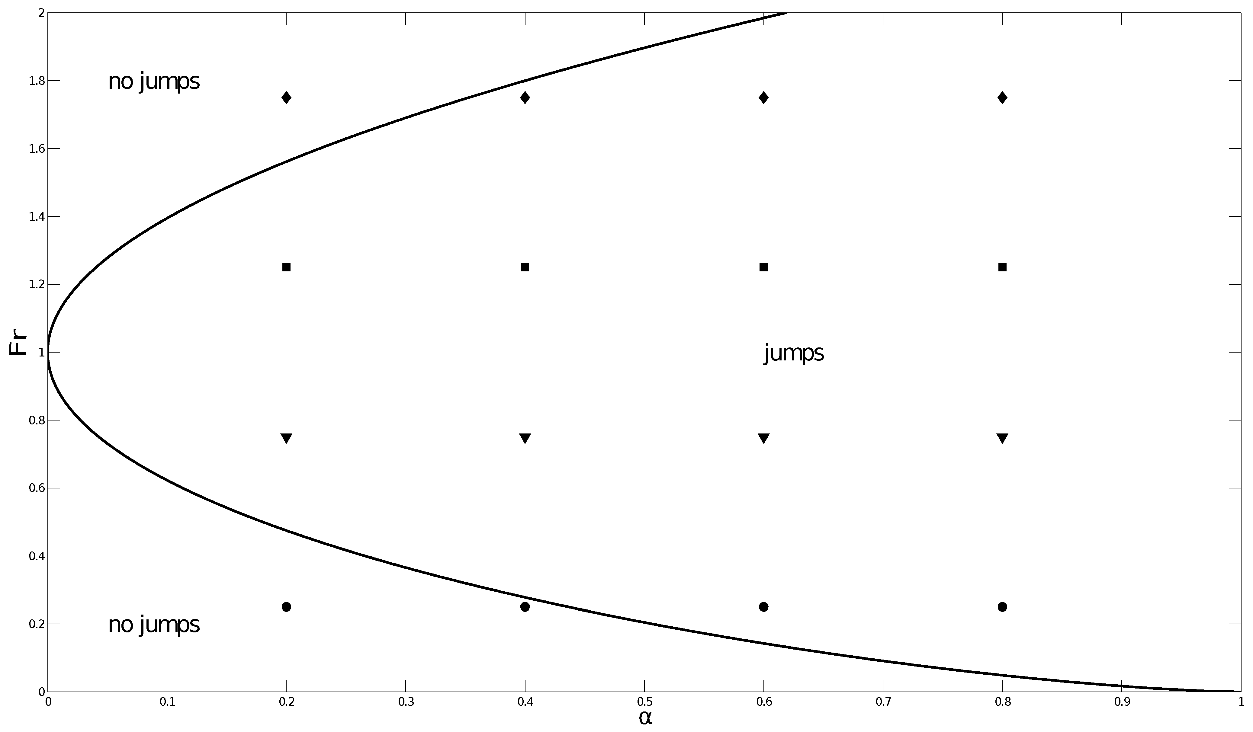
5.1. Analysis of the Parameters $\lambda$ and $\beta$

The results presented above show how the prediction of the simple SW model can differ from those of the complete NS one. The cause of this discrepancy must be sought in the approximation made to simplify the model. These approximations concern the terms $\beta (t,x)$ and $\lambda (t,x)$, considered equal to 1 in the SW model. Now, these parameters can actually be explicitly predicted from the full NSM simulations. In order to understand why the results of the two models differ, thus we report in Figure 7 and Figure 8, respectively, the $\beta$ and $\lambda$ parameters as functions of the streamwise coordinate, for the different values of $F_n$ and $\alpha$. Each figure has four subplots in which four curves obtained at different blocking factors and same equilibrium Froude numbers are compared.

The parameter $\beta$, is the variance of the velocity profile plus 1, as defined in Equation (18). It is therefore equal to 1 when the variance is null, i.e., for a flat profile. A fluid in turbulent motion presents a logarithmic mean velocity profile whose variance is of order $5\%$, so that approximating $\beta$ equal to one is acceptable. However, when a viscous fluid is studied, this approximation is not suitable anymore. The velocity profile of a Newtonian fluid with a free boundary is a half parabola, whose variance is $20\%$, leading to $\beta =1.2$. This value is valid for the unperturbed flow but, in the proximity of the weir, the profile and consequently $\beta$ can change.

In Figure 7, the pattern of the factor $\beta$ is shown. Far from the obstacle the fluid reaches the equilibrium state, and so $\beta$ reaches the value $1.2$ for the considered laminar flow. The distance at which the equilibrium is reached depends on both $\alpha$ and $F_n$. The smaller the $\alpha$, the less $\beta$ changes. This is obvious because having a smaller blocking factor is equivalent to having a smaller obstacle. On the other hand, the bigger the $\alpha$, the more the velocity profile, and so $\beta$, changes, with two pics prior and after the obstacle, the maximum being always located downstream the obstacle. This increase in $\beta$ can be associated with the two circulation cells downstream and upstream the obstacle. Moreover, a minimum value of $\beta$ is obtained at the top of the obstacle, with a value $\beta \simeq 1$. At this position, the velocity profile is therefore close to a bulk flow, i.e., a flat velocity profile.

The other parameter $\lambda$, defined in Equation (19), is the ratio between the wall friction of the flow and the wall friction of the equilibrium state, which is equal to one if the bottom is smooth. $\lambda$ is equal to 1 if the laminar flow reaches its equilibrium profile. Nevertheless, if the fluid flows over a rough bottom, the resulting motion can be complex, leading to vortices and secondary flows which reduce the similarity between the NS and SW model, that is only valid under the assumption of slowly variable bottom.

In Figure 8, the pattern of $\lambda$ is shown. As for $\beta$, far upstream and downstream the obstacle, the equilibrium value, $\lambda =1$ is reached. The non-dimensional dissipation parameter $\lambda$ has, for all the considered cases, the following shape: it approaches 1 for $x\to \pm \infty$, has two minima at the beginning and end points of the obstacle and a maximum slightly upstream the top of the obstacle.

5.2. Apparent Bottom for the SW Model

Since there does not seem to be a simple way to parameterize $\beta$ and $\lambda$ to enhance the SW model in the present configuration, we choose $\beta =1$ and $\lambda =1$, which is the common assumption in the SW model, and seek to adjust an “apparent bottom” denoted by $Z_a\left(x\right)$. We thus consider the SW system

$$\left\{\begin{array}{c}{\displaystyle q=U_a{h}_a}\hfill \\ {\displaystyle U_a\frac{d{U}_a}{dx}+gcos\theta \frac{d{h}_a}{dx}=-gcos\theta \frac{d{Z}_a}{dx}+gsin\theta -3\nu \frac{U_a}{h_a^2}.}\hfill \end{array}\right.$$

(27)

where $h_a\left(x\right)$ and $U_a\left(x\right)$ are the new variables in response to the apparent bottom $Z_a$. Knowing the steady surface height $Z_s\left(x\right)$ computed from the NS model, we want to adjust $Z_a\left(x\right)$ in order to satisfy the constraint $Z_s\left(x\right)=Z_a\left(x\right)+h_a\left(x\right)$. The apparent bottom is thus the solution of the equations

$$\left\{\begin{array}{c}{\displaystyle Z_a=Z_s-h_a}\hfill \\ {\displaystyle \frac{d{h}_a}{dx}=\frac{g}{q^2}\left(cos\theta \frac{d{Z}_s}{dx}-sin\theta \right)h_a^3+\frac{3\nu }{q}.}\hfill \end{array}\right.$$

(28)

The shape of the apparent bottoms $Z_a\left(x\right)$ are displayed in Figure 9 for the 16 considered configurations. All these shapes are smoother than the actual semi-circular profile and exhibit a maximum located downstream the actual one. The apparent bottom solution clearly captures the main features of the free-surface, derived from the NS model, which are disregarded in the SW model close to the obstacle. In particular, the obtained apparent bottom roughly incorporates both the actual obstacle and the complex flow cells induced by its presence. FromEquation (28), we can see that the slope of the apparent bottom is proportional to the slope of the free-surface. Since for this combination of Froude numbers and blocking factors the free surface profile is wavy, in agreement with [53,54,55,56], this explains the apparent bottom pattern in Figure 8a–c. The concept of apparent bottom seems, however, more intuitive for the case $F_n=1.75$ since regular bumpy shapes are observed in Figure 8d.

6. Conclusions

We have compared the steady solutions of a two phase flow on a titled bottom with a semi-circular obstacle for both the 2D Navier–Stokes (NS) equations and the Shallow Water (SW) equations. For constant values of the geometrical Reynolds number $R_g=26$ and the lower fluid viscosity $\nu$, different values of the angle $\theta$ and the flux discharge q have to be chosen in order to explore 16 values of the couple $(F_n,\alpha )$ while keeping the normal Reynolds number $R_n$ small enough to ensure that the flow remains laminar.

The numerical simulations have shown that the sharpness of the obstacle is responsible for the existence of hydraulic jumps and trans-critical regimes for the SW model that were not observed for the NS model. This rapid variation of the bottom is also responsible for departure of the velocity profile from the parabolic shape, that exists far upstream and downstream the obstacle, which has been quantified due to the departure of $\beta \left(x\right)$ and $\lambda \left(x\right)$, respectively, the velocity variance and dissipation parameters, from their asymptotic values.

The physical reason behind the differences between the SW and NS results is the static pressure modeling. In the SW model, the pressure is considered o be hydrostatic, as in Equation (15). This approximation is reasonable, however around a rough topography the static pressure departs from hydrostatic values. Because in first approximation, the total pressure, i.e., static plus dynamic, is constant, this significantly affects the fluid kinetic energy around the obstacle. This is reflected in both the changes in $\beta \left(x\right)$ and $\lambda \left(x\right)$. In particular, the dissipation increases sharply upstream the obstacle, while the kinetic energy increases downstream it. The increase dissipation around the obstacle and the increased velocity gradient, i.e., velocity variance, both prevent the occurrence of hydraulic jumps in the NS model.

We have shown that the SW model could give better prediction of stratified flows over macro-rugosities by replacing the topography with a smoother, apparent bottom. The determination of the apparent bottom is based on an exact match between the free surface height of both the NS and SW equations, which constitutes the main advantage of this approach, since NS is a more reliable model than SW, as well as its novelty. However, in an attempt to reproduce the Stokes waves, for a certain range of Froude numbers and blocking factors, this procedure adds further bumps on the bottom. This makes the shape of the apparent bottom more complex than the original topography, which is an undesirable feature.

The main conclusions of this work are quantified as follows:

• The SW and the NS model give different results in the presence of a sharp topography;
• The two models differs most for supercritical conditions, i.e., $F>1$;
• The local velocity profile variance $\beta \left(x\right)$ and the local dissipation coefficient $\lambda \left(x\right)$ have been deemed responsible for the diferences between the two models;
• The apparent bottom obtained from Equation (28) is able to reproduce free-surface profiel;
• However, this procedure is highly sensitive to any ripples at the interface and the apparent bottom shape is very complex, especially in subcritical (F < 1) flows.

Further studies are required to remove the additional rugosities by imposing artificial constraints on the regularity of the apparent bottom. This would lead to a systematic determination of an apparent bottom for different types of “macro-rugosities”. Furthermore, this study is limited to a two-dimensional, highly viscous flow. Future investigation should deal with more realistic, three-dimensional turbulent flows.

References

1. Abdullah, A.J. A proposed mechanism for the development of the eye of a hurricane. J. Meteorol. 1954, 11, 189–195. [Google Scholar] [CrossRef] [Green Version]
2. Tepper, M. The Application of the Hydraulic Analogy to Certain Atmospheric Flow Problems; Number 35; US Government Printing Office: Washington, DC, USA, 1952.
3. Benton, G.S. The occurrence of critical flow and hydraulic jumps in a multi-layered fluid system. J. Meteorol. 1954, 11, 139–150. [Google Scholar] [CrossRef] [Green Version]
4. Houghton, D.D.; Kasahara, A. Nonlinear shallow fluid flow over an isolated ridge. Commun. Pure Appl. Math. 1968, 21, 1–23. [Google Scholar] [CrossRef]
5. Jiang, Q.; Smith, R.B. Gravity wave breaking in two-layer hydrostatic flow. J. Atmos. Sci. 2003, 60, 1159–1172. [Google Scholar] [CrossRef]
6. Tokyay, T.; Constantinescu, G.; Gonzalez-Juez, E.; Meiburg, E. Gravity currents propagating over periodic arrays of blunt obstacles: Effect of the obstacle size. J. Fluids Struct. 2011, 27, 798–806. [Google Scholar] [CrossRef]
7. Sonder, I.; Zimanowski, B.; Büttner, R. Non-Newtonian viscosity of basaltic magma. Geophys. Res. Lett. 2006, 33. [Google Scholar] [CrossRef]
8. Greve, R.; Blatter, H. Dynamics of Ice Sheets and Glaciers; Springer Science & Business Media: Berlin/Heidelberg, Germany, 2009. [Google Scholar]
9. Coussot, P. Rheometry of Pastes, Suspensions, and Granular Materials: Applications in Industry and Environment; John Wiley & Sons: Hoboken, NJ, USA, 2005. [Google Scholar]
10. Benney, D. Long waves on liquid films. J. Math. Phys. 1966, 45, 150–155. [Google Scholar] [CrossRef]
11. Melville, W.; Helfrich, K.R. Transcritical two-layer flow over topography. J. Fluid Mech. 1987, 178, 31–52. [Google Scholar] [CrossRef] [Green Version]
12. Grimshaw, R.; Smyth, N. Resonant flow of a stratified fluid over topography. J. Fluid Mech. 1986, 169, 429–464. [Google Scholar] [CrossRef]
13. Dias, F.; Vanden-Broeck, J.M. Steady two-layer flows over an obstacle. Philos. Trans. R. Soc. Lond. A Math. Phys. Eng. Sci. 2002, 360, 2137–2154. [Google Scholar] [CrossRef]
14. Dias, F.; Vanden-Broeck, J.M. Two-layer hydraulic falls over an obstacle. Eur. J. Mech.-B/Fluids 2004, 23, 879–898. [Google Scholar] [CrossRef]
15. Cooker, M.; Peregrine, D.; Vidal, C.; Dold, J. The interaction between a solitary wave and a submerged semicircular cylinder. J. Fluid Mech. 1990, 215, 1–22. [Google Scholar] [CrossRef] [Green Version]
16. Zhang, Y.; Zhu, S. Subcritical, transcritical and supercritical flows over a step. J. Fluid Mech. 1997, 333, 257–271. [Google Scholar] [CrossRef] [Green Version]
17. Havelock, T. The method of images in some problems of surface waves. Proc. R. Soc. Lond. Ser. A Contain. Pap. Math. Phys. Character 1927, 115, 268–280. [Google Scholar]
18. Lamb, H. Hydrodynamics; Cambridge University Press: Cambridge, UK, 1932. [Google Scholar]
19. Long, R.R. Some aspects of the flow of stratified fluids. Tellus A 1955, 7, 341–357. [Google Scholar] [CrossRef]
20. Lawrence, G. Steady flow over an obstacle. J. Hydraul. Eng. 1987, 113, 981–991. [Google Scholar] [CrossRef]
21. Long, R.R. Some Aspects of the Flow of Stratified Fluids: II. Experiments with a Two-Fluid System. Tellus 1954, 6, 97–115. [Google Scholar] [CrossRef]
22. Baines, P.G. A unified description of two-layer flow over topography. J. Fluid Mech. 1984, 146, 127–167. [Google Scholar] [CrossRef]
23. Armi, L. The hydraulics of two flowing layers with different densities. J. Fluid Mech. 1986, 163, 27–58. [Google Scholar] [CrossRef] [Green Version]
24. Fadda, D.; Raad, P.E. Open channel flow over submerged obstructions: An experimental and numerical study. J. Fluids Eng. 1997, 119, 906–910. [Google Scholar] [CrossRef]
25. Armi, L.; Farmer, D. Maximal two-layer exchange through a contraction with barotropic net flow. J. Fluid Mech. 1986, 164, 27–51. [Google Scholar] [CrossRef]
26. Baines, P. Upstream influence and Long’s model in stratified flows. J. Fluid Mech. 1977, 82, 147–159. [Google Scholar] [CrossRef] [Green Version]
27. Chunrong, L.; Aode, H.; Wenju, M. Numerical and experimental investigation of flow over a semicircular weir. Acta Mech. Sin. 2002, 18, 594–602. [Google Scholar] [CrossRef] [Green Version]
28. Younis, B.A.; Przulj, V.P. Prediction of hydrodynamic loading on a mini TLP with free surface effects. Ocean Eng. 2006, 33, 181–204. [Google Scholar] [CrossRef]
29. Dewangan, N.; Das, A.; Das, P. Free surface flow over a bump with hydraulic jump. In Proceedings of the 4th BSME-ASME International Conference on Thermal Engineering, Dhaka, Bangladesh, 27–29 December 2008. [Google Scholar]
30. Lin, L.; Li, Y.C.; Bin, T.; Bing, C. Numerical simulation of turbulent free surface flow over obstruction. J. Hydrodyn. Ser. B 2008, 20, 414–423. [Google Scholar]
31. Muzaferija, S.; Peri’c, M. Computation of free-surface flows using the finite-volume method and moving grids. Numer. Heat Transf. 1997, 32, 369–384. [Google Scholar] [CrossRef]
32. Lonyangapuo, J.; Elliott, L.; Ingham, D.; Wen, X. Identification of the shape of the bottom surface of a channel from a given free surface profile. WIT Transactions on Modelling and Simulation; WIT Press: Southampton, UK, 1998; pp. 81–90. [Google Scholar]
33. Lonyangapuo, J.; Elliott, L.; Ingham, D.; Wen, X. Retrieval of the shape of the bottom surface of a channel when the free surface profile is given. Eng. Anal. Bound. Elem. 1999, 23, 457–470. [Google Scholar] [CrossRef]
34. Lonyangapou, J.; Elliott, L.; Ingham, D.; Wen, X. A boundary integral technique for solving for an unknown bottom surface given a free surface fluid flow. Int. Ser. Adv. Bound. Elem. 1999, 25, 365–374. [Google Scholar]
35. Lonyangapuo, J.; Elliott, L.; Ingham, D.; Wen, X. Flow in channels over rigid obstacles of unknown shape. In Proceedings of the Second UK Conference on Boundary Integral Methods; Wrobel, L.C., Chandler-Wilde, S., Eds.; Brunel University Press: Brunel, UK, 1999; pp. 165–176. [Google Scholar]
36. Lonyangapuo, J.; Elliott, L.; Ingham, D.; Wen, X. Use of an extremal functional in solving for an unknown bottom surface given a free surface profile. Eng. Anal. Bound. Elem. 2000, 24, 17–30. [Google Scholar] [CrossRef]
37. Lonyangapuo, J.; Elliott, L.; Ingham, D.; Wen, X. Solving free surface fluid flow problems by the minimal kinetic energy functional. Int. J. Numer. Methods Fluids 2001, 37, 577–600. [Google Scholar] [CrossRef]
38. Zhang, J.; Wang, Y.P. A method for inversion of periodic open boundary conditions in two-dimensional tidal models. Comput. Methods Appl. Mech. Eng. 2014, 275, 20–38. [Google Scholar] [CrossRef]
39. Butler, T.; Graham, L.; Estep, D.; Dawson, C.; Westerink, J. Definition and solution of a stochastic inverse problem for the Manning’sn parameter field in hydrodynamic models. Adv. Water Resour. 2015, 78, 60–79. [Google Scholar] [CrossRef] [PubMed] [Green Version]
40. Zaron, E.D. On the observability of bottom topography from measurements of tidal sea surface height. Ocean Model. 2016, 102, 55–63. [Google Scholar] [CrossRef] [Green Version]
41. Guinot, V.; Sanders, B.F.; Schubert, J.E. Dual integral porosity shallow water model for urban flood modelling. Adv. Water Resour. 2017, 103, 16–31. [Google Scholar] [CrossRef] [Green Version]
42. Brisset, P.; Monnier, J.; Garambois, P.A.; Roux, H. On the assimilation of altimetric data in 1D Saint–Venant river flow models. Adv. Water Resour. 2018, 119, 41–59. [Google Scholar] [CrossRef] [Green Version]
43. Monnier, J.; Zhu, J. Inference of the bottom topography in anisothermal mildly-sheared shallow ice flows. Comput. Methods Appl. Mech. Eng. 2019, 348, 954–977. [Google Scholar] [CrossRef] [Green Version]
44. Garambois, P.A.; Larnier, K.; Monnier, J.; Finaud-Guyot, P.; Verley, J.; Montazem, A.S.; Calmant, S. Variational estimation of effective channel and ungauged anabranching river discharge from multi-satellite water heights of different spatial sparsity. J. Hydrol. 2020, 581, 124409. [Google Scholar] [CrossRef]
45. Al-Ghosoun, A.; El Moçayd, N.; Seaid, M. A surrogate model for efficient quantification of uncertainties in multilayer shallow water flows. Environ. Model. Softw. 2021, 144, 105176. [Google Scholar] [CrossRef]
46. Boico, V.F.; Therrien, R.; Højberg, A.L.; Iversen, B.V.; Koganti, T.; Varvaris, I. Using depth specific electrical conductivity estimates to improve hydrological simulations in a heterogeneous tile-drained field. J. Hydrol. 2022, 604, 127232. [Google Scholar] [CrossRef]
47. Hirt, C.; Nichols, B. Volume of fluid (VOF) method for the dynamics of free boundaries. J. Comput. Phys. 1981, 39, 201–225. [Google Scholar] [CrossRef]
48. Angelino, M.; Boghi, A.; Gori, F. Numerical solution of three-dimensional rectangular submerged jets with the evidence of the undisturbed region of flow. Numer. Heat Transf. Part A Appl. 2016, 70, 815–830. [Google Scholar] [CrossRef] [Green Version]
49. Di Venuta, I.; Petracci, I.; Angelino, M.; Boghi, A.; Gori, F. Numerical simulation of mass transfer and fluid flow evolution of a rectangular free jet of air. Int. J. Heat Mass Transf. 2018, 117, 235–251. [Google Scholar] [CrossRef] [Green Version]
50. Kurganov, A.; Levy, D. Central-upwind schemes for the Saint-Venant system. ESAIM Math. Model. Numer. Anal. 2002, 36, 397–425. [Google Scholar] [CrossRef] [Green Version]
51. Kurganov, A.; Petrova, G. A second-order well-balanced positivity preserving central-upwind scheme for the Saint-Venant system. Commun. Math. Sci. 2007, 5, 133–160. [Google Scholar] [CrossRef] [Green Version]
52. Angelino, M.; Xia, H.; Moratilla-Vega, M.; Page, G. Far-field noise prediction of round and serrated jets with increasingly refined grids. In Proceedings of the 22nd AIAA/CEAS Aeroacoustics Conference, Lyon, France, 30 May–1 June 2016; p. 3047. [Google Scholar]
53. Forbes, L.K.; Schwartz, L.W. Free-surface flow over a semicircular obstruction. J. Fluid Mech. 1982, 114, 299–314. [Google Scholar] [CrossRef]
54. Forbes, L.K. Free-surface flow over a semicircular obstruction, including the influence of gravity and surface tension. J. Fluid Mech. 1983, 127, 283–297. [Google Scholar] [CrossRef]
55. Forbes, L. Critical free-surface flow over a semi-circular obstruction. J. Eng. Math. 1988, 22, 3–13. [Google Scholar] [CrossRef]
56. Zhang, Y.; Zhu, S. Open channel flow past a bottom obstruction. J. Eng. Math. 1996, 30, 487–499. [Google Scholar] [CrossRef]
57. Pratt, L. A note on nonlinear flow over obstacles. Geophys. Astrophys. Fluid Dyn. 1983, 24, 63–68. [Google Scholar] [CrossRef]
Figure 1. Diagram of the 16 numerical experiments for α { 0.2 , 0.4 , 0.6 , 0.8 } and F n { 0.25 , 0.75 , 1.25 , 1.75 } . Theoretical critical curve α = 1 ( 3 / 2 ) F n 2 / 3 + ( 1 / 2 ) F n 2 in plain lines. Circles (◯): sub-critical regimes. Diamonds (⋄): super-critical regimes. Squares (□): trans-critical regimes. Up-triangles (△). Down-triangles (▽).
Applsci 12 02476 g001
Figure 2. Computational grid around the obstacle.
Applsci 12 02476 g002
Figure 3. Free surface height Z s ( z ) computed by Navier–Stokes (dotted) and Shallow Water (plain black) model for F n = 0.25 and (a) α = 0.8 , (b) α = 0.6 , (c) α = 0.4 and (d) α = 0.2 .
Applsci 12 02476 g003
Figure 4. Free surface height Z s ( z ) computed by Navier–Stokes (dotted) and Shallow Water (plain black) model for F n = 0.75 and (a) α = 0.8 , (b) α = 0.6 , (c) α = 0.4 and (d) α = 0.2 .
Applsci 12 02476 g004
Figure 5. Free surface height Z s ( x ) computed by Navier–Stokes (dotted) and Shallow Water (plain) model for F n = 1.25 and (a) α = 0.8 , (b) α = 0.6 , (c) α = 0.4 and (d) α = 0.2 .
Applsci 12 02476 g005
Figure 6. Free surface height Z s ( x ) computed by Navier–Stokes (dotted) and Shallow Water (plain) model for F n = 1.75 and (a) α = 0.8 , (b) α = 0.6 , (c) α = 0.4 and (d) α = 0.2 .
Applsci 12 02476 g006
Figure 7. Shape factor β ( x ) at different blocking factors: α = 0.8 (dotted), α = 0.6 (dash dotted), α = 0.4 (dashed) and α = 0.2 (plain). (a) F n = 0.25 , (b) F n = 0.75 , (c) F n = 1.25 and (d) F n = 1.75 .
Applsci 12 02476 g007
Figure 8. Dissipation factor λ ( x ) at different blocking factors: α = 0.8 (dotted), α = 0.6 (dash dotted), α = 0.4 (dashed) and α = 0.2 (plain). (a) F n = 0.25 , (b) F n = 0.75 , (c) F n = 1.25 and (d) F n = 1.75 .
Applsci 12 02476 g008
Figure 9. Apparent bottom Z a ( x ) at different blocking factors: α = 0.8 (dotted), α = 0.6 (dash dotted), α = 0.4 (dashed) and α = 0.2 (plain). (a) F n = 0.25 , (b) F n = 0.75 , (c) F n = 1.25 , (d) F n = 1.75 .
Applsci 12 02476 g009