Simulation of Track-Soft Soil Interactions Using a Discrete Element Method

Abstract

With the development of unmanned tracked vehicles, soil model predictions of soft terrains are becoming more essential. In order to accurately simulate the interaction characteristics between soil particles and the track, soil modeling with a discrete element method (DEM) is proposed. Volume-based scaled-up modeling of DEM soil particles and the calibration of DEM input parameters were investigated as a feasible approach to realizing many particle calculations. Calibration of DEM input parameters can solve the distortions between actual and DEM particle sizes. Cohesion and friction parameters of the scaled-up soil particle model were recalibrated by the shape accumulated through the virtual design of the experiment. Soil DEM particles were scaled up to 1 mm spherical particles, and recalibrated DEM parameter values were used to match the actual accumulated soil shape. Three calibrated scaled-up soil models were used for the shear stress–displacement DEM simulation of a track segment, and the mean absolute percentage error (MAPE) was less than 11% compared with the actual shear stress–displacement test. The parameter value of soil traction performance empirical model of a tracked vehicle is modified according to the soil shear stress–displacement DEM simulation. Comparative analysis was performed for travel test results of a tracked vehicle; the relative error of the soil traction prediction results to actuals was less than 16.8%. This showed that the volume-based particle scaling technique is an effective DEM for the mechanical simulation of soil.

1. Introduction

With the development of special unmanned tracked vehicles, more unmanned tracked vehicles are being used in soft soil environments, i.e., river dredging tracked equipment. In order to estimate the trafficability of soft soil, the research focus of the terramechanics of tracked vehicles has gradually shifted to the detailed modeling of soft soil.

In soft ground conditions, the tractive performance of a tracked vehicle is determined by the interaction between the track and the soil. Previous researchers studied the effect of the geometry of the track segment on tractive performance [1,2], such as grouser height, pitch, thickness and pitch-to-height ratio. Most of the contemporary research has focused on land soil. For soft soil with a high moisture content, the traditional method is still used to test the mechanical properties of the soil. Due to the high sinkage of soft soil, traditional soil shear tests are unsuitable.

Most previous studies on the interaction between soil and track have been performed through a soil bin in the laboratory or on an actual field. With the development of computer technology, the application of DEM to interaction problems in terramechanics has become popular. DEM was first proposed and introduced into the study of vehicle terramechanics [3]. Nakashima used a two-dimensional DEM to simulate soil, and verified the effect of track traction in combination with a soil bin test [4]. Du assessed the mechanical properties of soft ground with low moisture, low viscosity and high friction [5]. Peters established a vehicle-terrain simulation model based on the DEM and proved the accuracy of traditional drawbar-pull tests [6]. Zhou proposed a systematic and accurate discrete element modeling method for sandy roads [7]. The verification results showed that the modeled interactions between track and sandy ground based on DEM simulations were consistent with the results of the actual soil bin test. For fine soil particles, a major disadvantage of DEM simulation in practical applications is the challenge of modeling very small particles; it is computationally impossible and impractical to calculate every particle of true size.

In order to reduce the amount of calculation, a feasible method is to apply scaled-up particle technology to DEM simulation. At present, the scaled-up particle method is more commonly used in DEM simulation [8,9,10]. If all particle sizes are scaled up by a constant factor, but the material properties remain the same, the dynamics of the granular system will be altered [11]. Thus, DEM parameter calibrations are the key challenge for the scaled-up particle method.

Many contemporary scholars have focused on the parameter calibration method of DEM simulation. DEM calibration consists of the careful choice of the material input parameters needed to reflect the real behavior of the particles in the numerical simulation. Careful calibration is the basis for achieving predictive results. The methods of parameter calibration include the angle of repose (AOR) test, penetration test, compression test and shear test [12,13,14,15,16]. Due to the large number of material attributes to be set, most of the calibration is focused on selected parameters. More calibration procedures for the DEM parameters have been developed to reduce computational effort [17,18,19].

In the studies reported above, the DEM was applied to the terramechanics of tracked vehicles; the main research objects are limited to land soil and sand. However, the applicability of DEM simulation to soft soil is uncertain. The objectives of this study were: (1) to calibrate scaled-up particle contact parameters consistent with the mechanical properties of soft soil; (2) to validate the shear properties of the scaled-up particle model and (3) to corroborate the soil traction performance of the tracked vehicle according to the modified soil shear DEM simulation.

2. Material and Methods

2.1. Parameters Calibration of Scaled-Up Particles

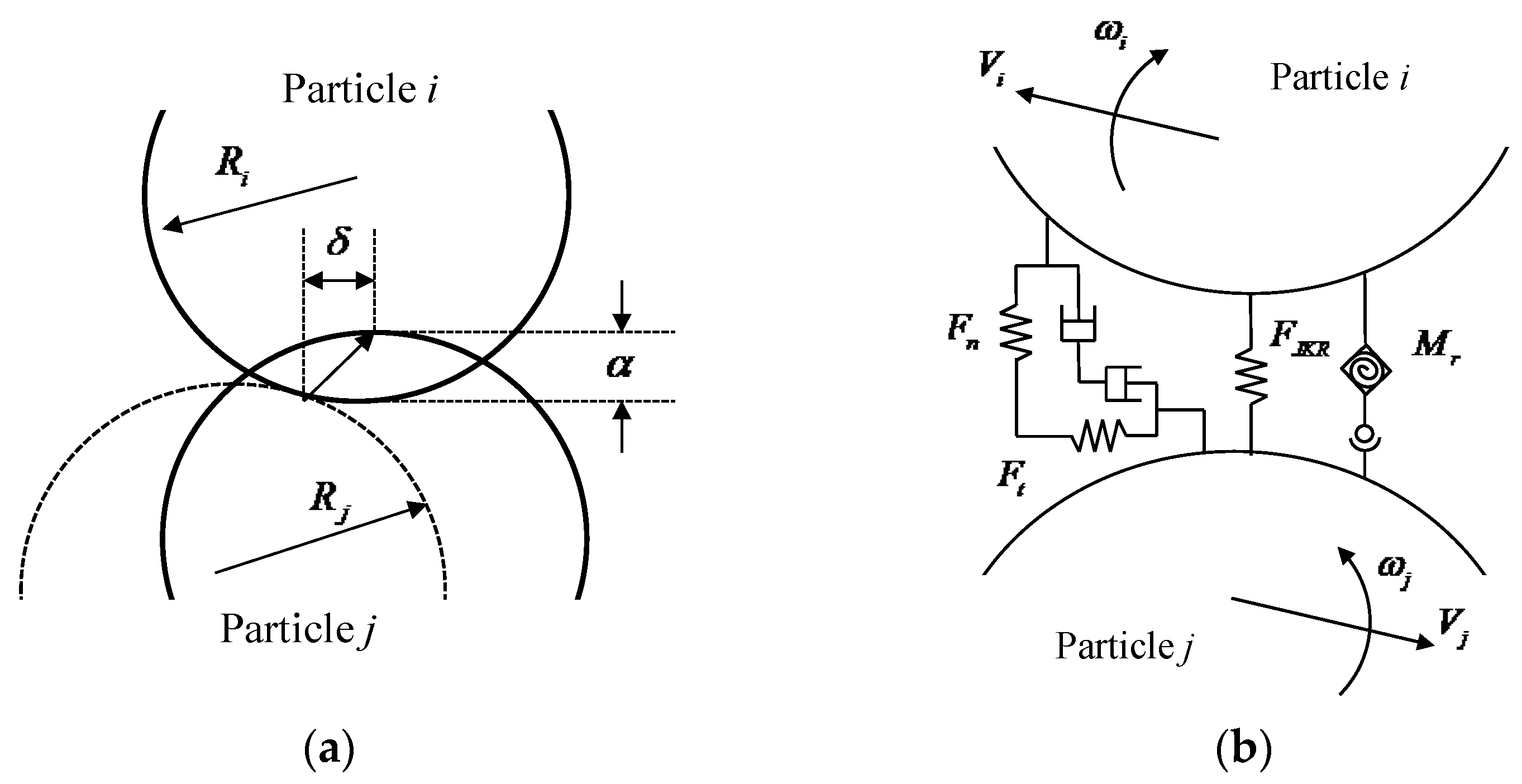
2.1.1. JKR Model in the DEM

The Johnson–Kendall–Roberts (JKR) contact model was developed from the Hertz–Mindlin contact model. The Hertz–Mindlin contact model is the basis of DEMs, and is accurate and efficient. Here, the Hertz contact model is applied for the calculation of normal forces [20], and the Mindlin contact model is applied for the calculation of tangential forces [21]. As a supplement, the damping component should be considered based on the damping coefficient and recovery coefficient [22]. Additionally, tangential friction and rolling friction should complied with the Mohr–Coulomb law and the contact-independent directional constant torque model [23].

Based on the theory of the Hertz–Mindlin model, the load analysis for interactions among particles is derived as five categories: normal elastic force, normal damping force, tangential elastic force, tangential damping force and rolling friction. For soft soil with a high moisture content, the liquid bridge force has a great influence on the interaction between particles, which is ignored by the Hertz–Mindlin model. In the JKR model, the normal elastic force is developed and modified, with a comprehensive analysis of cohesive forces caused by the action of water. The JKR model is a method of contact simulation for cohesive particles, which can be used to simulate the cohesive effects among wet particles, as shown in Figure 1.

In order to characterize the cohesion between particles, a new parameter of surface energy is introduced to calculate the cohesive forces. The equivalent JKR normal elastic force can be expressed as [24]:

$$F_{JKR}=-4\sqrt{\pi \gamma E^{*}}{\alpha }^{\raisebox{1ex}{$3$}\!\left/ \!\raisebox{-1ex}{$2$}\right.}+\frac{4E^{*}}{3R^{*}}{\alpha }^3,$$

(1)

$$\delta =\frac{{\alpha }^2}{R^{*}}-\sqrt{\raisebox{1ex}{$4\pi \gamma \alpha $}\!\left/ \!\raisebox{-1ex}{$E^{*}$}\right.},$$

(2)

where $E^{*}$ is the equivalent elastic modulus, $R^{*}$ is the equivalent radius, $\gamma$ is the surface energy, $\delta$ is the overlap and $\alpha$ is the interaction parameter.

The equivalent elastic modulus and equivalent radius could be calculated with Hertz [20] model.

$$E^{*}=\frac{(1-v_i^2)}{E_i}+\frac{(1-v_j^2)}{E_j},$$

(3)

$$\frac{1}{R^{*}}=\frac{1}{R_i}+\frac{1}{R_j},$$

(4)

where $E_i$ and $E_j$ are the elastic moduli of two contacted particles; ${\upsilon }_i$ and ${\upsilon }_j$ are the Poisson ratios of two contact particles and $R_i$ and $R_j$ are the radii of two contacted particles.

In the JKR contact model, even if the particles are not in contact, cohesion forces still occur between particles. The maximum clearance that produces non-zero cohesion force between particles can be expressed as [24]:

$${\delta }_c=\frac{{\alpha }_c^2}{R^{*}}-\sqrt{\raisebox{1ex}{$4\pi \gamma a_c$}\!\left/ \!\raisebox{-1ex}{$E^{*}$}\right.},$$

(5)

$${\alpha }_c={\left[\frac{9\pi \gamma R^{*2}}{2E^{*}}\left(\frac{3}{4}-\frac{1}{\sqrt{2}}\right)\right]}^{\frac{1}{3}}$$

(6)

2.1.2. Calibration of the JKR Model Parameters

Riverbed surface soil is a complex sediment with a high moisture content. With the increase in moisture content, the soil presents a plastic state, fluid plastic state and flow state. The different content of sand in the soil will also change the soil characteristics. In this paper, the clay and sand were collected from the Huai River, a representative river in northern China, used as the in situ data for tests and simulations. As a supplement, three kinds of clay and sand mixed soil, 1# (75:25 wt.%), 2# (50:50 wt.%) and 3# (25:75 wt.%), were applied to soil shear tests and DEM simulations. The wet densities of mixed soil 1#, 2# and 3# were 1.54 g cm⁻³, 1.65 g cm⁻³ and 1.74 g cm⁻³, respectively.

The discretization of DEM particle sizes and their distribution which comprises particle sizes of natural soils is very complex and computationally prohibitive. The main particle size composition of soil can be screened by standard assays. Based on the main particle size of the soil, soil particles are assumed to be uniformly distributed. Under the assumed condition, the scaled-up particle is set to 1 mm in the DEM simulation, which can simplify and accelerate the calculation [25].

In this paper, standard screening and drying experiments were applied to test the physical properties of soil. First, the standard screening of 300 mesh and 200 mesh was used to identify clay particles of sizes 0.05–0.075 mm. Meanwhile, the standard screening of 35 mesh and 18 mesh was used to identify soil particles of sizes 0.5–1 mm. Second, the collected soil was placed in a graphite crucible and warmed in the incubator at 100 °C. The weight of the crucible was measured every 24 h until the error of two measurements was less than 1%. The wet density, dry density and moisture content (water mass fraction) of the soil could be obtained through calculations, with the results shown in

Table 1. The characteristics of clay and sand.

Property	Clay	Sand
Particle size (mm)	0.05–0.075	0.5–1
Wet density (g cm−3)	1.45	1.97
Dry density (g cm−3)	0.67	1.63
Moisture content (%)	91	21

.

As shown in Table 1, particle sizes of clay and sand were less than 0.075 mm and 1 mm, respectively, and modeling soil based on actual particle sizes requires a significant amount of computing resources. The optimal method is to increase the size of soil particles proportionally and derive the same mechanical properties as the actual soil particles by setting appropriate parameters. In this study, for comprehensive consideration of the actual particle size and the calculation ability of computer, the clay and sand particles were set as spherical particles 1 mm in size in the DEM simulation [26]. The characteristic coefficients of particle interactions were determined by comparing the real experiment with the simulation [15,16].

Three types of parameters were indispensable in the JKR contact model [14]:

(1)

The intrinsic parameters of particles, including wet density, Poisson ratio, shear modulus and particle size, are basic parameters and can be measured by the test. The parameters are shown in Table 2;

(2)

The contact parameters of particles, including the static friction coefficient and rolling friction coefficient, are friction characteristic parameters and can be measured by tests or calibrated by simulations. The friction between particles is calculated according to the friction characteristic parameters, and the specific calculation method refers to the Hertz–Mindlin model [20,21];

(3)

The JKR models specific particle parameters, i.e., surface energy, which is a cohesive characteristic parameter and is difficult to measure. However, it can be calibrated by DEM simulation. The cohesive force between particles is calculated according to the cohesive characteristic parameters, as shown in Equation (1).

Table 2. DEM parameters used in the simulations.

Property	Value	Source
Shear modulus of clay (MPa)	2.85 × 104	Ucgul [27]
Poisson’s ratio of clay	0.3	Asaf [28]
Coefficient of restitution of clay–clay	0.4	Wang [29]
Coefficient of restitution of clay–PVC	0.4	Wang [29]
Shear modulus of sand (MPa)	4.3 × 104	Asaf [28]
Poisson’s ratio of sand	0.3	Asaf [28]
Coefficient of restitution of sand–sand	0.6	Das [30]
Restitution coefficient of sand–PVC	0.6	Das [30]
Density of PVC (g cm−3)	1.3	Suggested by EDEM [31]
Elastic modulus of PVC (MPa)	2.41 × 103	Suggested by EDEM [31]
Poisson’s ratio of PVC	0.383	Suggested by EDEM [31]

Table 2. DEM parameters used in the simulations.

Property	Value	Source
Shear modulus of clay (MPa)	2.85 × 104	Ucgul [27]
Poisson’s ratio of clay	0.3	Asaf [28]
Coefficient of restitution of clay–clay	0.4	Wang [29]
Coefficient of restitution of clay–PVC	0.4	Wang [29]
Shear modulus of sand (MPa)	4.3 × 104	Asaf [28]
Poisson’s ratio of sand	0.3	Asaf [28]
Coefficient of restitution of sand–sand	0.6	Das [30]
Restitution coefficient of sand–PVC	0.6	Das [30]
Density of PVC (g cm−3)	1.3	Suggested by EDEM [31]
Elastic modulus of PVC (MPa)	2.41 × 103	Suggested by EDEM [31]
Poisson’s ratio of PVC	0.383	Suggested by EDEM [31]

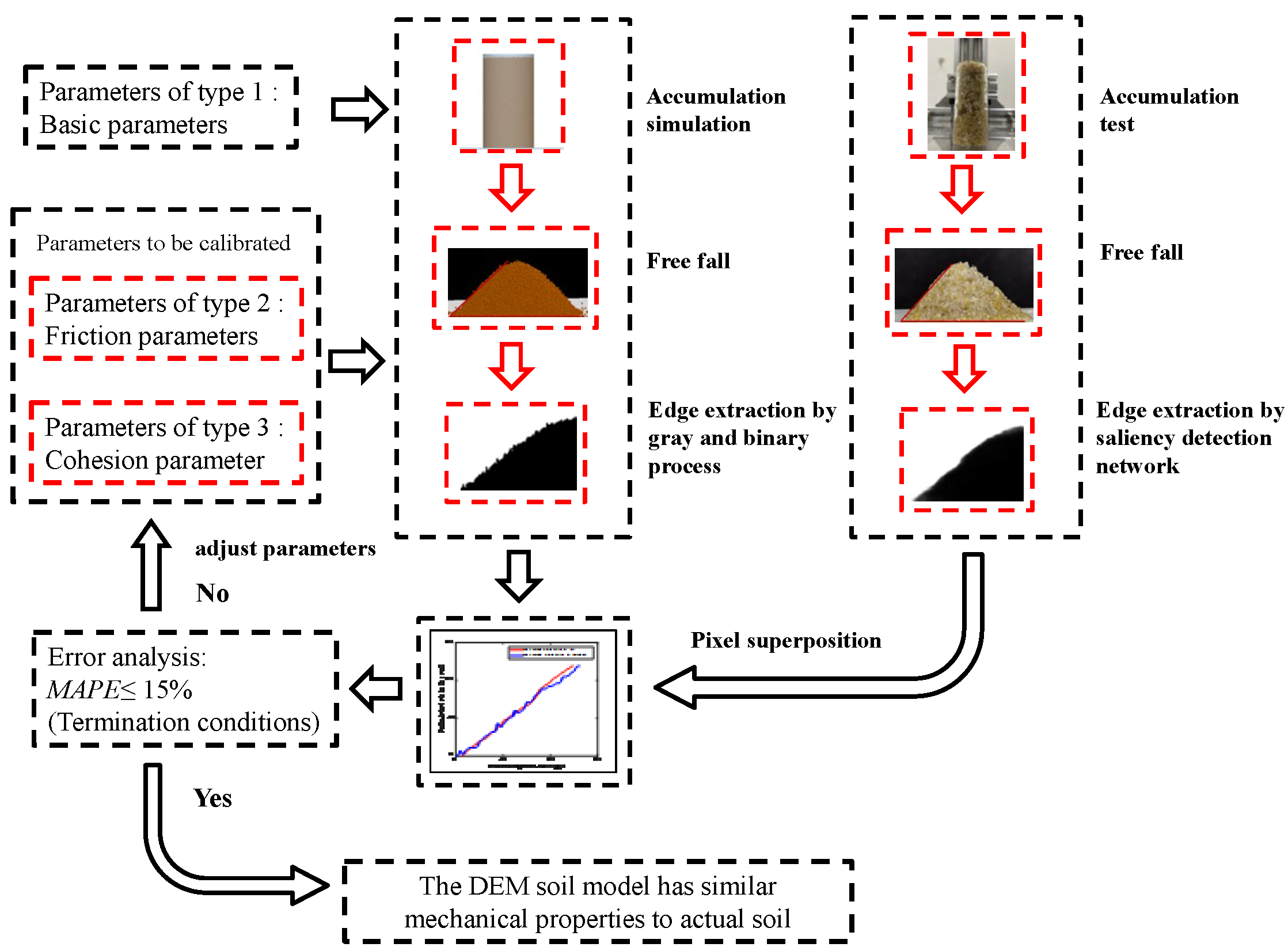
2.1.3. Parameter Calibration by the Accumulation Test

For soil with a high moisture content, the repose angle of soil particles is affected by the friction and cohesion of particles. Thus, it is necessary to recalibrate the characteristic parameters of scaled-up particles.

In this paper, the lifting cylinder test was used to calibrate the soil repose angle. First, the cylinder filling soil particles was placed on the surface of the test platform and raised vertically at a speed of 5 mm s⁻¹ by a screw device driven by a stepper motor (57BL55S06). The soil particles fell freely through and formed a conical pile on the base plate. Second, the same experimental parameters were set in the DEM simulation. The basic contact parameters of particles are shown in Table 2. Finally, the contact parameters that needed to be calibrated were finally confirmed by comparing the accumulation test and simulation. The dimensions of the cylinder and the cylinder model established in the EDEM software with the same size are shown in Figure 2.

Trial-and-error methods are feasible to change the parameters and comparison results constantly until the simulation results conform to the actual experimental results. Different accumulations were measured through the above experimental steps. Accumulation tests and DEM simulations were carried out, as shown in Figure 3.

As shown in Figure 3e, the repose angle of sand particles is mainly determined by friction and can be measured directly. Unlike the formation principle of the repose angle of sand particles, clay is a kind of soil with a small internal friction angle. The repose angle of clay particles is mainly determined by the cohesion, which causes the irregular shape accumulation and is difficult to measure accurately.

To accurately measure the characteristic parameters of mixed soil and analyze the accumulation of mixed soil with different proportions of sand, a method of image edge extraction and pixel superposition through a saliency detection network and grey-binary processing was proposed with MATLAB software. A schematic diagram of the soil contact parameter calibration method is shown in Figure 4.

2.2. Interaction between Soil and Track

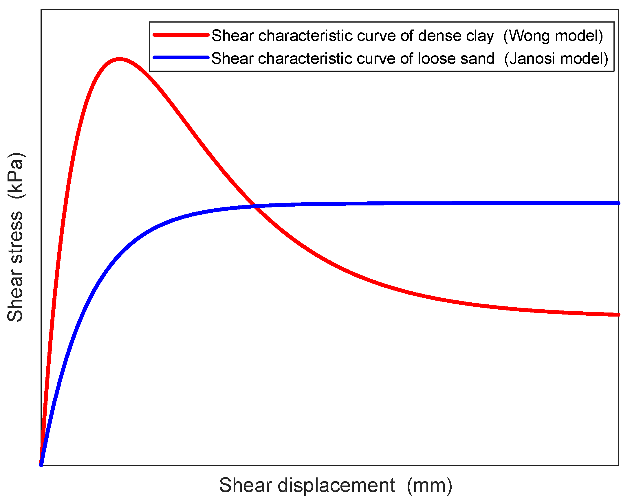
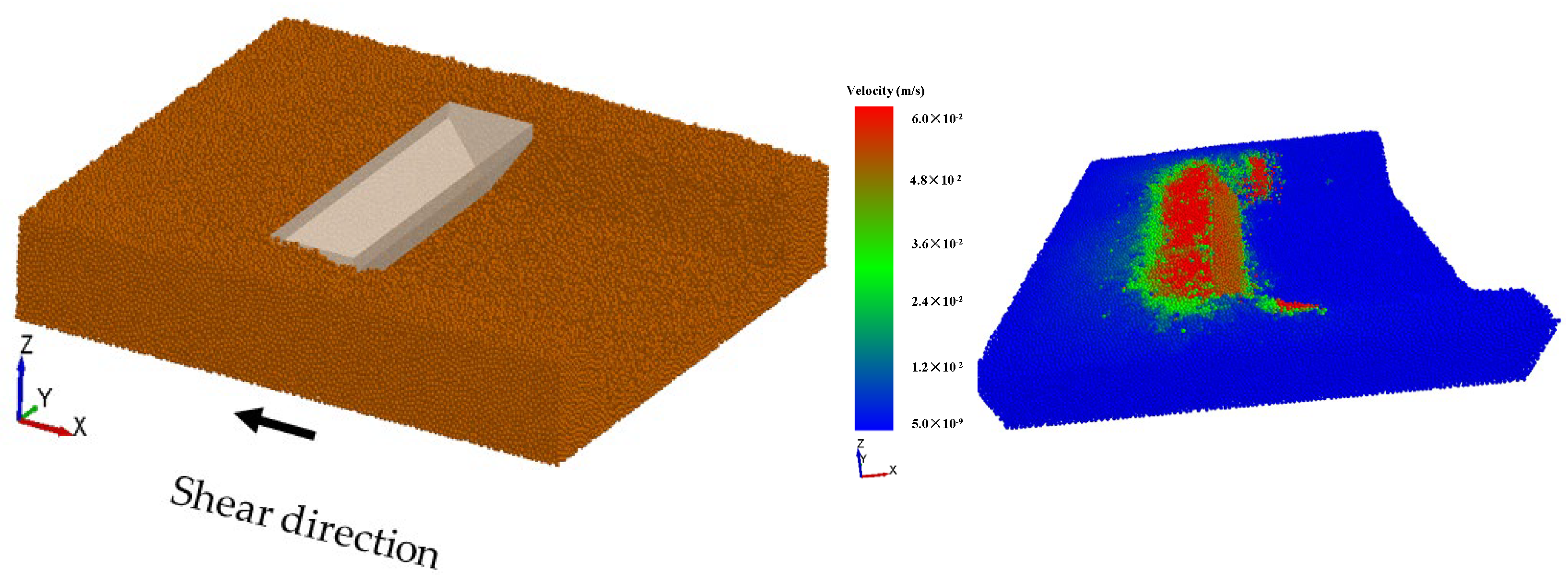
2.2.1. Shear Stress–Displacement Model

The locomotion of a tracked vehicle on the surface of soil is mainly based on the shear forces that develop between the track links and surface soil in the longitudinal direction. Soil conditions have significant effects on tractive performance.

According to prior surveys and tests, the characteristics of clay are similar, in that shear stress initially increases sharply and reaches a “hump” of maximum shear stress ${\tau }_{\max }$ at a particular shear displacement, and then decreases and approaches a relative constant residual value ${\tau }_{res}$ with further increases in shear displacement, which relationship may be characterized by the following empirical equation proposed by Wong [32,33]:

$${\tau }_{Clay}={\tau }_{\max }{K}_r\{1+[\frac{1}{K_r(1-e^{-1})}]\cdot e^{1-j(x)/K_w}\}\cdot (1-e^{-j(x)/K_w})$$

(7)

where ${\tau }_{\max }$ is the maximum shear stress, $K_w$ is the shear displacement where the maximum shear stress occurs and $K_r$ is the ratio of residual shear stress to maximum shear stress.

However, sand has shear stress characteristics which increase rapidly and then approach a relatively constant value, for which the relationship may be characterized by the following empirical equation proposed by Janosi [34]:

$${\tau }_{Sand}={\tau }_{\max }(1-e^{-j(x)/K}),$$

(8)

where K is the shear displacement where the maximum shear stress occurs. Variation trends in shear stress of different types of soil are shown in Figure 5.

2.2.2. Shear Stress–Displacement Test

The shear test apparatus consisted of an electrical step motor which produced a constant horizontal displacement in the soil bin (600 mm × 300 mm × 300 mm) with a soil height of 30 mm and a resistance strain force sensor, as shown in Figure 6. The force sensor (DYMH-106) is a strain sensor with a comprehensive error of less than 0.3% F.S. To ensure the track segment shear stability process, the motor speed was set to 0.05 m/s and the sampling frequency was set to 50 Hz. The test platform was connected to a computer for data acquisition and processing. It should be noted that after each stress–displacement test, the soil and water were thoroughly mixed and pre-compressed according to the grounding contact pressure of the tracked vehicle. Schematic diagrams of the experimental platform and track segment. Parameters of the track segment structural dimensions are shown in

Table 3. Parameters of track segment structural dimension.

Parameter	Track Segment
Material	PVC Rigid
Length (mm)	80
Width (mm)	60
Grouser height (mm)	12

.

In shear stress–displacement tests and simulations, clay, sand and mixed soil 2# were applied to shear stress–displacement test, as shown in Figure 7.

2.2.3. Shear Stress–Displacement DEM Simulation and Modification Process

According to the soil shear stress–displacement test, the virtual soil bin in the DEM simulation was set to 130 mm × 120 mm × 22 mm containing 400,000 soil particles, considering the computer’s capability. The computer’s CPU was an Intel 7700 processer with four cores and eight threads, and the simulation time was 42 h.

The virtual soil bin and the shear simulation process between the soil and track segment with DEM simulation are shown in Figure 8 and Figure 9, respectively. The number of soil particles that produced the bulldozing effect above the track segment was about 165,000, and the soil volume is 85.3 cm³. The movement speed of soil particles on the track segment was about 0.036 m s⁻¹, which was less than the movement speed of the track segment 0.05 m s⁻¹. The difference in the velocity among soil particles led to the bulldozing resistance of the track segment.

In order to remove the bulldozing resistance caused by soil accumulation, the calculation domain of the particles was adjusted. The soil shear test was performed based on adjusting the particle calculation domain. The virtual soil bin and simulation of the shear process between the clay and track segment with the EDEM software are shown in Figure 10. In the virtual shear simulation, there was no soil accumulation in front of the track segment.

The image of the motion state of clay particles was derived, as shown in Figure 10. The motion of soil particles near the inner wall of the soil bin was almost static, which indicated that soil particles near the inner wall did not participate in the shear process, and the size of the soil bin was suitable. The motion state of clay particles participating in the shear simulation was about 0.045 m s⁻¹, which is consistent with the moving speed of the track segment—0.05 m s⁻¹. According to the motion of the particles in front of the track segment, there were about 23,500 particles, and the effective soil volume involved in the shear process was 24 cm³. Compared with the soil shear DEM simulation without modification, the volume of accumulated soil causing the error was 60 cm³. This shows that the error caused by soil accumulation could not be ignored.

The mean absolute percentage error (MAPE) was applied to evaluate the accuracy of the simulation model. When the MAPE value was close to zero, the DEM simulation model was more consistent with reality.

$$MAPE=\frac{100\%}{n_s}{\displaystyle \sum _{i=1}^n\left|\frac{{\widehat{y}}_i-y_i}{y_i}\right|},$$

(9)

where n_s is the number of samples, y_i is the test value of samples and ${\widehat{y}}_i$ is the simulation value of samples.

2.3. Verification of Traction Performance of Soft Soil

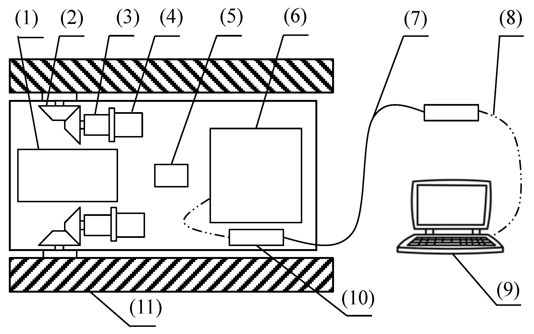
2.3.1. Traction Calculation and Travel Test of Tracked Vehicle

The shear stress at any point of contact can be determined based on the hypothesis that contact pressure is distributed uniformly. With Equation (7), the traction force F_t can be deduced by the integral [32,33]:

$$\begin{array}{ll}{F}_t=& \{(Ac+4hLc)+W\cdot \tan \varphi [1+0.64(\frac{h}{b}\mathrm{arccot}(\frac{h}{b})]\}\cdot K_r\hfill \\ & \{[1+\frac{K_w}{iL}(e^{-(iL/K_w)}-1)]-(\frac{e}{K_r(e-1)}-1)\cdot \frac{K_w}{2iL}(2e^{1-(iL/K_w)}-e^{1-(2iL/K_w)}-e)\}\hfill \end{array}$$

(10)

where A is the contact area between track and soil. b is the track width, L is the contact length between track and soil, h is the grouser height, W is the gravity of tracked vehicle and i is the slip.

In order to verify the accuracy of the DEM and evaluate the soil tractive performance, external load estimated by the motor current was carried out. Firstly, the corresponding relationship between motor current and load torque was analyzed based on the motor characteristics test data. Secondly, the soil tractive performance could be calculated according to the load torque of the motor and the structure of the tracked vehicle. A schematic diagram of the tracked vehicle is shown in Figure 11.

In order to ensure the accuracy of the tests, a track segment in the shear stress–displacement test was applied to the tracked vehicle. Travel tests were performed in a soil bin (2.7 m × 0.8 m × 0.6 m) containing clay of about 0.3 m in height, as shown in

Table 4. Specifics of the tracked vehicle.

Parameter	Value
Length, width and height of tracked vehicle (m)	$0.6\times 0.48\times 0.3$
Weight of tracked vehicle (kg)	24
Interface length of track (m)	0.32

. The specifics of the tracked vehicle are shown in Figure 11.

Tracked vehicle travel tests were performed on a clay terrain, as shown in Figure 12. In the tracked vehicle travel test, the rotation speed of both motors was set to 50 rpm, and the tracked vehicle speed was 0.028 m s⁻¹. Limited by the soil bin, the tracked vehicle’s total distance and test time were about 1.7 m and 60 s, respectively.

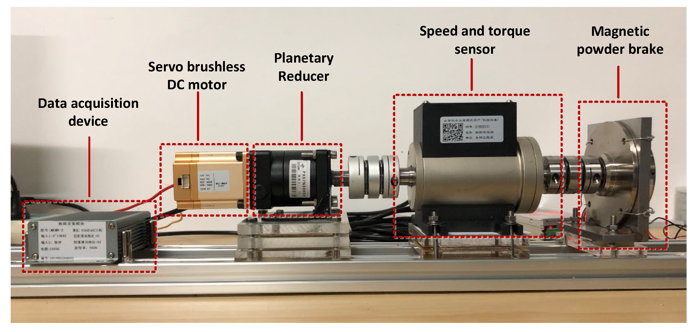
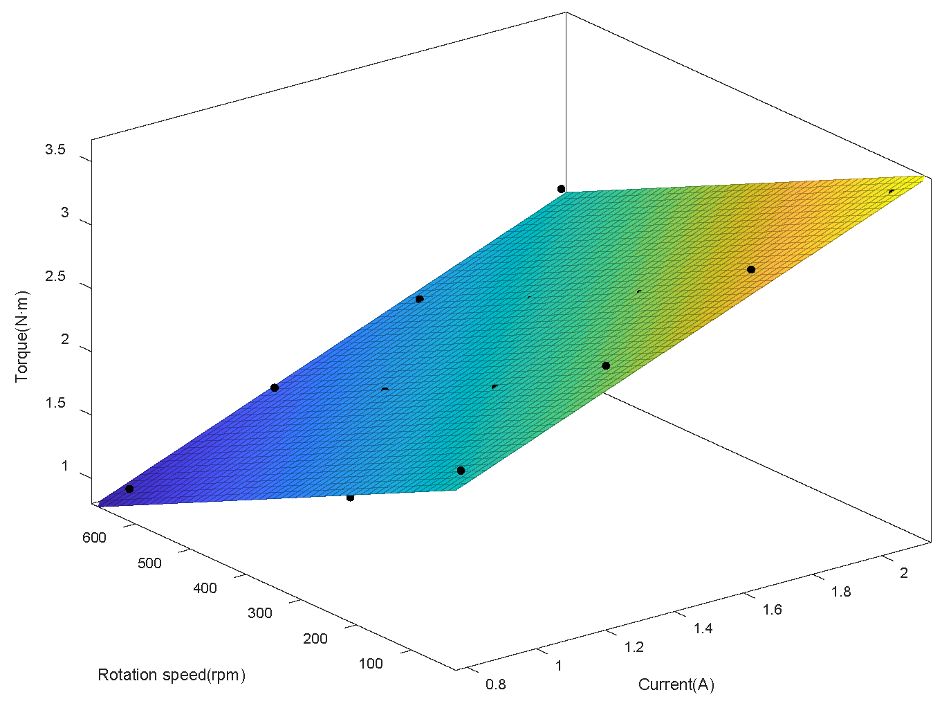
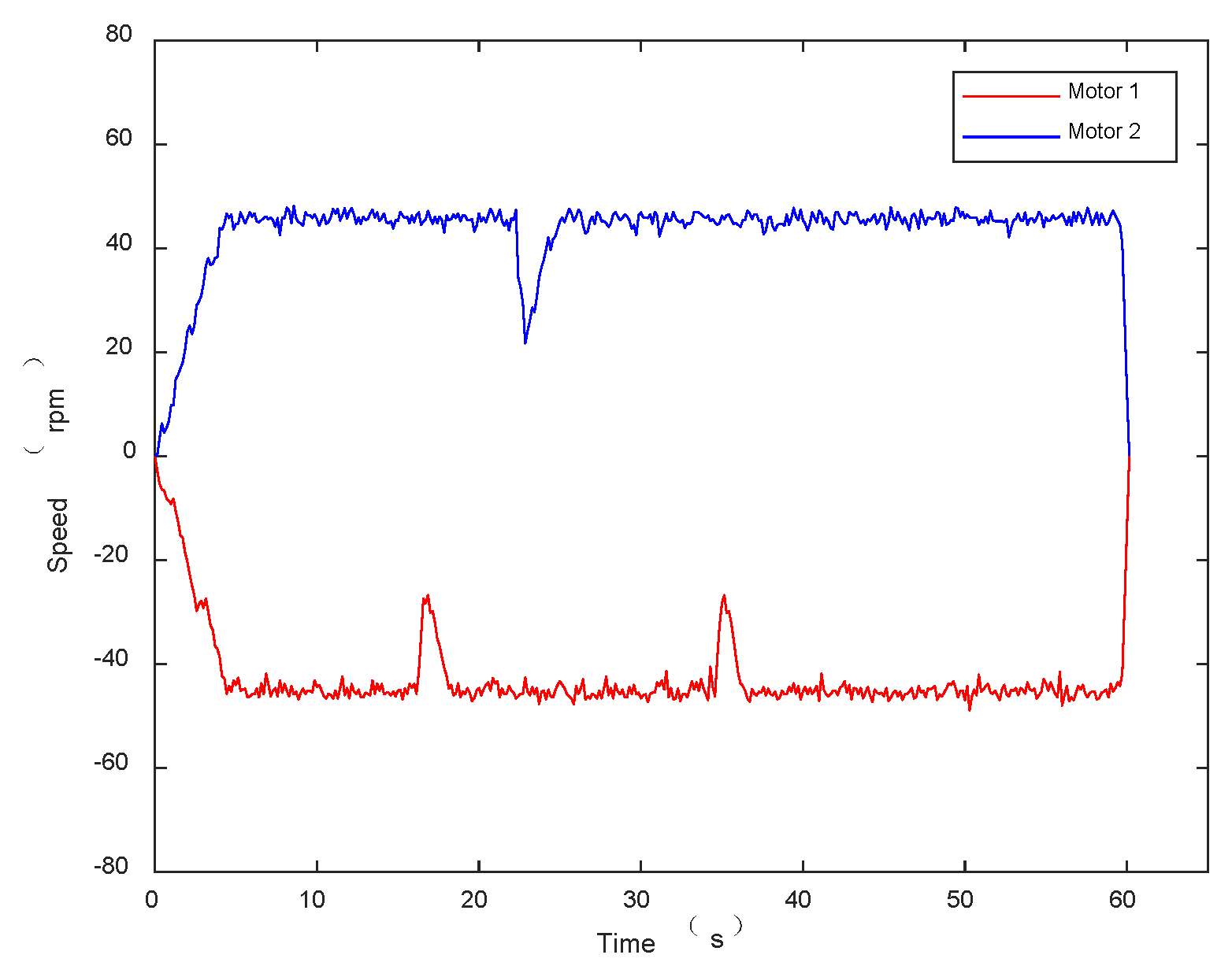
2.3.2. Drive Motor Characteristic Tests

A motor characteristics test platform was designed, as shown in Figure 13. The test platform was equipped with a high-precision DC brushless servo motor, a planetary gear reducer, a torque sensor, and a magnetic powder brake. The specifics of the motor test platform are shown in

Table 5. Specifics of the motor test platform.

Servo brushless DC motor	Power up to 100 W; Rotational speed up to 1000 rad min−1; Torque up to 0.96 Nm Min resolution 1 mA
Planetary reducer	Reduction ratio 1:6
Speed and torque sensor	Measuring range 0–100 Nm Measurement accuracy < 0.1% F.S Min resolution 0.01 Nm
Magnetic powder brake	Resistance force moment up to 6 Nm

.

For a comprehensive consideration of traveling speed and capacity of the tracked vehicle, the sampling frequency of the motors was set at 10 Hz, and the motor power was set at 60 W. The relationship between the motor current and external load torque was obtained at a series of certain rotational speeds. The relationship between the motor current and external load torque is shown in Figure 14.

According to the test data, the relationships between the torque, speed and current of the motor are considered comprehensively, and the load torque T can be expressed as:

$$T=1.14+1.07I-0.002n,$$

(11)

where T is the load torque of the motor, I is the current of the motor and n is the rotary speed of the motor.

3. Results and Discussion

3.1. Mechanical Property Verification of Scaled-Up Particles

The accumulated shape, obtained by pixel superposition, is shown in Figure 15. With the increase in sand particle content, the accumulation height of soil decreases gradually, and the flow state becomes more obvious. When the content of sand particles is low, the interaction between soil particles is mainly a cohesive force. However, with the increase in the content of sand particles, pore water film between the clay particles is broken. This leads to the molecular force between clay particles becoming smaller, and soil cohesion also decreases. Moreover, when the soil is mainly composed of sand particles, the pores between sand particles are filled with clay particles. These high-moisture-content clay particles affect lubrication, which causes the soil to become a flow state.

As analyzed above, the AOR of clay particles and sand particles is different. The simulation of soil accumulation can reproduce the accumulation test results with the properly adjusted friction and cohesion parameters of soil. Friction and cohesion characteristics of different soils are shown in Figure 16.

The above results indicate that both cohesive and frictional properties exist in clay particles. However, friction is the main characteristic of sand. Meanwhile, the friction characteristic curves of soils with different compositions are nonlinear. Clay and sand are modeled as spherical particles, which means that the friction parameters between particles are set as larger than that of the actual situation. The significance of accumulation is to explore appropriate contact parameters according to different soil compositions.

It should be noted that the friction and cohesion characteristics in this study were based on a soil particle size of 1 mm. Additionally, the calibration of friction and cohesion are greatly affected by particle size. The coordinate ordinate axes represent the friction coefficient and surface energy of soil particles based on spherical scaled-up particles.

3.2. Soil Shear Characteristic Verification of Track Segment

3.2.1. Comparative Analysis of the Results of the Soil Shear Test and DEM Simulation

As the shear displacement of the track segment increases, more soil is accumulated in front of the track segment (marked by the red circle in Figure 7). Additionally, the test data collected by the force sensor include the shear force between the track segment and the soil and the resistance caused by the soil accumulation in front of the track segment. The shear stress–displacement test result has great errors without completely removing the influence of “bulldozing”. However, it is impossible to completely remove the accumulated soil in front of the track segment in the test. As shown in Figure 17, the shear stress values of clay test data increase continuously.

The accumulated soil in front of the track segment produced a great impact in the measurement and was difficult to remove completely. However, the accumulated soil in front of the track segment could be effectively removed by changing the calculation domain in DEM, which could modify the shear relationship model of the soil and track segment accurately.

The MAPE of clay, sand and mixed soil were 7.5%, 11% and 9%, which indicated that the prediction model is accurate and effective. Shear stress–displacement fitting data from the test and simulation are shown in Figure 18.

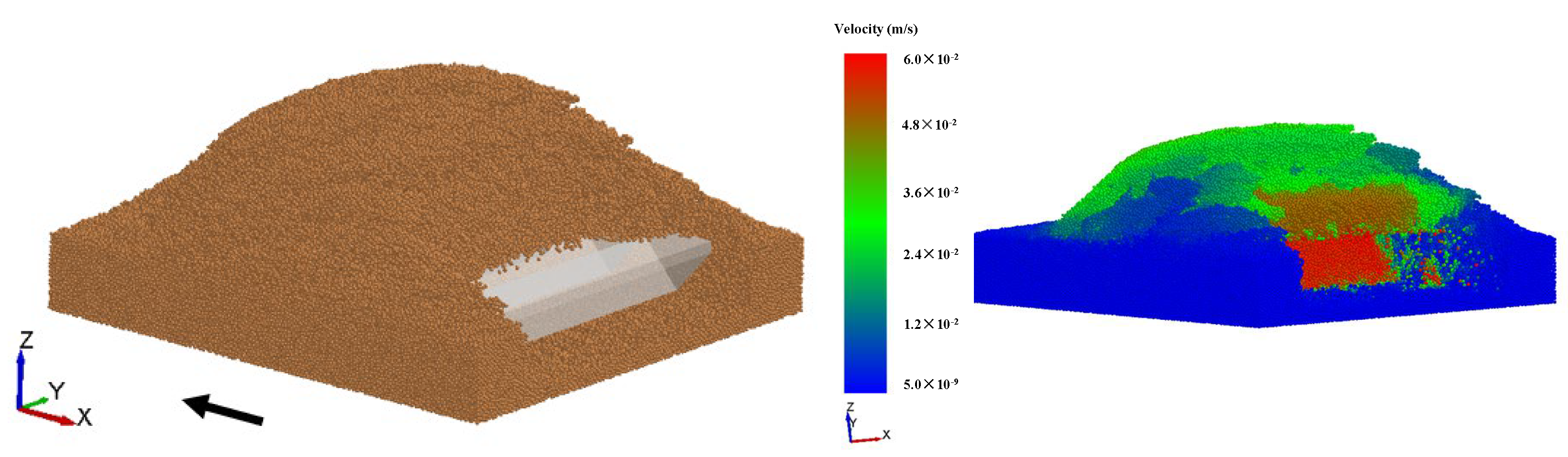
3.2.2. Modified DEM Simulation of Track Segment Shear Process

The stress along the shear direction of the track segment was converted into a line graph, as shown in Figure 19. Through the comparative analysis of Figure 18 and Figure 19, it can be seen that the bulldozing resistance caused by soil accumulation in front of the soil plate was effectively eliminated. The force variation trend was more consistent with the shear regularity of the clay and track segment. The stress trend in the track segment following the shear regularity could also be obtained from the sand and mixed soil simulations. The key parameters in the classical model are summarized in Figure 19 and detailed in

Table 6. Parameters of the shear stress–displacement model.

Parameter	Clay	Mixed Soil 2#	Sand
${\tau }_{\max }$ (kPa)	5.28	1.65	3.5
$K_r$	0.53	0.52	–
$K_w$, $K$ (m)	0.013	0.016	0.02

.

Comparisons of the classical model and simulation fitting are shown in Figure 20; the stress variation in the DEM simulation is similar to that of the classical model. Meanwhile, the maximum shear stress and residual shear stress in the DEM simulation are consistent with the classical model. According to the shear stress–displacement data and fitting curve, the necessary parameters of the shear stress–displacement model could be obtained, as shown in Table 6.

However, as the maximum shear stress changed to the residual shear stress, errors were obvious between the simulation and classical model. The pores between the scaled-up particles in the DEM simulation were larger than the actual pores of soil particles, which mean that the particles in the DEM simulation are easier to compress and rebound. In the terramechanics of the tracked vehicle, maximum shear stress, residual shear stress and location of maximum stress determined the accuracy of soil traction calculation. Shown in Figure 20, the values of the maximum shear stress, residual shear stress and location of the maximum stress fitted well in the DEM simulation and classical model. Errors between the simulation and classical model will not affect the derivation of soil traction of the track.

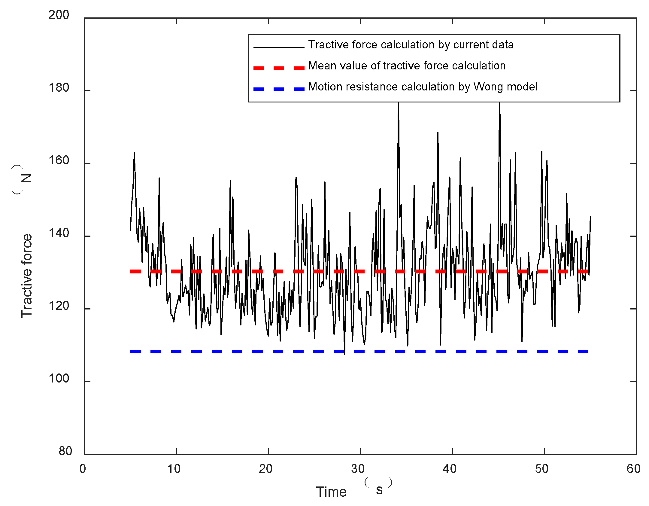
3.3. Soft Soil Traction Verification

In order to reduce the influence of noise, the test data were applied with a moving average filter using the MATLAB software, as shown in Figure 21. The rotary encoder obtained the rotation speed signals of two motors, as shown in Figure 22. In the tracked vehicle travel tests, clay was difficult to mix uniformly, which caused the rotation speed signal to fluctuate at some positions.

In order to eliminate influences of motion state change to current measured values, the acceleration and deceleration processes were excluded when analyzing the test data. The valid interval of test data was selected as from 5 to 60 s. The external load was calculated according to the characteristic relationship formula of the valid interval, as shown in

Table 7. Parameters of motor characteristics.

Parameter	Motor 1	Motor 2
Average speed by measured (rpm)	45.6	46.2
Average current by measured (A)	1.12	1.08
Average torque by calculated (Nm)	2.25	2.18

.

According to the characteristic of the motor, the motor current was converted to external load torque, as shown in Figure 23. The external resistance forces estimated by the motor current data and Wong model (Equation (9)) were 130.2 N and 108.3 N, respectively. The relative error between the soil traction performance calculation based on the scaled-up particle DEM and actual value was 16.8%, which is suitable for engineering applications.

4. Conclusions

(1)

According to the actual particle size of clay and sand, the particles were scaled up to 1 mm for DEM simulations. Based on the scaled-up particle size, the cohesion and friction characteristic parameters were calibrated. Appropriate DEM input parameters of the scaled-up DEM particle could reproduce the soft soil accumulation shape with acceptable error.

(2)

Calibrated scaled-up DEM particles were used in the soil shear stress–displacement simulation. The shear stress–displacement DEM simulation results were in accordance with the mechanical response and trends in the soil shear stress–displacement tests.

(3)

The revised shear stress–displacement DEM simulation results were applied to the soil traction performance model calculation of the tracked vehicle. The relative error between the traction performance calculation result and the tracked vehicle travel test result was 16.8%, which proved that it is feasible to perform soft soil DEM simulations with the scaled-up particle method.

References

1. Hata, S.; Hosoi, T. On the effects of lug pitch upon the tractive effort about track-laying vehicles. Proc. Int. Conf. ISTVS 1981, 1, 255–262. [Google Scholar]
2. Muro, T.; Omoto, K.; Futamura, M. Traffic Performance of a bulldozer running on a weak terrain vehicle model test. Doboku Gakkai Ronbunshu 1988, 397, 151–157. [Google Scholar] [CrossRef] [Green Version]
3. Oida, A.; Ohkubo, S. Effect of tire lug cross section on tire performance simulated by distinct element method. In Proceedings of the 13th International Conference of ISTVS, Munich, Germany, 14–17 September 1999; pp. 345–352. [Google Scholar]
4. Nakashima, H.; Yoshida, T.; Wang, X.L.; Shimizu, H.; Miyasaka, J.; Ohdoi, K. Comparison of gross tractive effort of a single grouser in two-dimensional DEM and experiment. J. Terramech. 2015, 62, 41–50. [Google Scholar] [CrossRef]
5. Du, Y.; Gao, J.; Jiang, L.; Zhang, Y. Numerical analysis on tractive performance of off-road wheel steering on sand using discrete element method. J. Terramech. 2017, 71, 25–43. [Google Scholar] [CrossRef]
6. Peters, J.; Vahedifard, F.; Jelinek, B.; Mason, G.; Priddy, J. The discrete element method for vehicle-terrain analysis. In Proceedings of the 15th European-African Regional Conference of the International Society for Terrain-Vehicle Systems, Prague, Czech Republic, 9–11 September 2019. [Google Scholar]
7. Zhou, L.; Gao, J.; Hu, C.; Li, Q. Numerical simulation and testing verification of the interaction between track and sandy ground based on discrete element method. J. Terramech. 2021, 95, 73–88. [Google Scholar] [CrossRef]
8. Thakur, S.C.; Ooi, J.Y.; Ahmadian, H. Scaling of discrete element model parameters for cohesionless and cohesive solid. Powder Technol. 2016, 293, 130–137. [Google Scholar] [CrossRef] [Green Version]
9. Lommen, S.; Mohajeri, M.; Lodewijks, G.; Schott, D. DEM particle upscaling for large-scale bulk handling equipment and material interaction. Powder Technol. 2019, 352, 273–282. [Google Scholar] [CrossRef]
10. Mohajeri, M.J.; van Rhee, C.; Schott, D.L. Replicating cohesive and stress-history-dependent behavior of bulk solids: Feasibility and definiteness in DEM calibration procedure. Adv. Powder Technol. 2021, 32, 1532–1548. [Google Scholar] [CrossRef]
11. Pöschel, T.; Saluena, C.; Schwager, T. Scaling properties of granular materials. In Continuous and Discontinuous Modelling of Cohesive-Frictional Materials; Springer: Berlin/Heidelberg, Germany, 2001; pp. 173–184. [Google Scholar]
12. Deng, J.Y.; Hu, J.; Li, Q.D.; Li, H.L.; Yu, T.C. Simulation and experimental study on the subsoiler based on EDEM discrete element method. J. Chin. Agric. Mech. 2016, 37, 14–18. [Google Scholar]
13. Huang, Y.; Hang, C.; Yuan, M.; Wang, B.; Zhu, R. Discrete element simulation and experiment on disturbance behavior of sub soiling. Trans. Chin. Soc. Agric. Mach. 2016, 47, 80–88. [Google Scholar]
14. Xia, R.; Li, B.; Wang, X.; Li, T.; Yang, Z. Measurement and calibration of the discrete element parameters of wet bulk coal. Measurement 2019, 142, 84–95. [Google Scholar] [CrossRef]
15. Bahrami, M.; Naderi-Boldaji, M.; Ghanbarian, D.; Ucgul, M.; Keller, T. DEM simulation of plate sinkage in soil: Calibration and experimental validation. Soil Tillage Res. 2020, 203, 104700. [Google Scholar] [CrossRef]
16. Li, P.; Ucgul, M.; Lee, S.H.; Saunders, C. A new approach for the automatic measurement of the angle of repose of granular materials with maximal least square using digital image processing. Comput. Electron. Agric. 2020, 172, 105356. [Google Scholar] [CrossRef]
17. Roessler, T.; Richter, C.; Katterfeld, A.; Will, F. Development of a standard calibration procedure for the DEM parameters of cohesionless bulk materials–part I: Solving the problem of ambiguous parameter combinations. Powder Technol. 2019, 343, 803–812. [Google Scholar] [CrossRef]
18. Richter, C.; Roessler, T.; Kunze, G.; Katterfeld, A.; Will, F. Development of a standard calibration procedure for the DEM parameters of cohesionless bulk materials–Part II: Efficient optimization-based calibration. Powder Technol. 2020, 360, 967–976. [Google Scholar] [CrossRef]
19. Orefice, L.; Khinast, J.G. A novel framework for a rational, fully-automatised calibration routine for DEM models of cohesive powders. Powder Technol. 2020, 361, 687–703. [Google Scholar] [CrossRef]
20. Hertz, H. Ueber die Berührung fester elastischer Körper. J. Die Reine Angew. Math. 1882, 92, 156–171. [Google Scholar]
21. Mindlin, R.D.; Deresiewicz, H. Elastic spheres in contact under varying oblique forces. J. Applied Mech. 1953, 20, 327–344. [Google Scholar] [CrossRef]
22. Tsuji, Y.; Tanaka, T.; Ishida, T. Lagrangian numerical simulation of plug flow of cohesionless particles in a horizontal pipe. Powder Technol. 1992, 71, 239–250. [Google Scholar] [CrossRef]
23. Sakaguchi, H.; Ozaki, E.; Igarashi, T. Plugging of the flow of granular materials during the discharge from a silo. Int. J. Mod. Phys. B 1993, 7, 1949–1963. [Google Scholar] [CrossRef]
24. Johnson, K.L.; Kendall, K.; Roberts, A. Surface energy and the contact of elastic solids. Proc. R. Soc. Lond. A Math. Phys. Sci. 1971, 324, 301–313. [Google Scholar]
25. Tekeste, M.Z.; Way, T.R.; Syed, Z.; Schaferb, R.L. Modeling soil-bulldozer blade interaction using the discrete element method (DEM). J. Terramech. 2020, 88, 41–52. [Google Scholar] [CrossRef]
26. Tsuji, T.; Nakagawa, Y.; Matsumoto, N.; Kadono, Y.; Takayama, T.; Tanaka, T. 3-D DEM simulation of cohesive soil-pushing behavior by bulldozer blade. J. Terramech. 2012, 49, 37–47. [Google Scholar] [CrossRef]
27. Ucgul, M.; Fielke, J.M.; Saunders, C. Three-dimensional discrete element modelling of tillage: Determination of a suitable contact model and parameters for a cohesionless soil. Biosyst. Eng. 2014, 121, 105–117. [Google Scholar] [CrossRef]
28. Asaf, Z.; Rubinstein, D.; Shmulevich, I. Determination of discrete element model parameters required for soil tillage. Soil Tillage Res. 2007, 92, 227–242. [Google Scholar] [CrossRef]
29. Wang, D.; Wang, Y.; Yang, B.; Zhang, W.; Lancaster, N. Statistical analysis of sand grain/bed collision process recorded by high-speed digital camera. Sedimentolog 2008, 55, 461–470. [Google Scholar] [CrossRef]
30. Das, B.M.; Khing, K.H. Cyclic Load-Induced Settlement of Shallow Foundations on Geogrid-Reinforced Layered Soil. In Proceedings of the Seventh International Offshore and Polar Engineering Conference, International Society of Offshore and Polar Engineers, Honolulu, HI, USA, 25–30 May 1997. [Google Scholar]
31. EDEM. EDEM Theory Reference Guide; EDEM Solutions: Edinburgh, UK, 2011. [Google Scholar]
32. Wong, J.; Thomas, J. On the characterization of the shear stress-displacement relationship of terrain. J. Terramech. 1983, 19, 225–234. [Google Scholar] [CrossRef]
33. Wong, J.Y. Theory of Ground Vehicles, 3rd ed.; John Wiley & Sons, Inc.: Hoboken, NJ, USA, 2001; pp. 133–159. [Google Scholar]
34. Janosi, Z. The analytical determination of drawbar pull as a function of slip for tracked vehicles in defarmable soils. In Proceedings of the 1st ISTVS International Conference, Turin, Italy, 24–27 September 1961. [Google Scholar]
Figure 1. Schematic of the JKR contact model. (a) Particle–particle contact model; (b) particle–particle force/torque interactions.
Applsci 12 02524 g001
Figure 2. Bottomless cylinder in accumulation test and simulation.
Applsci 12 02524 g002
Figure 3. Soil accumulation test and DEM simulation. (a) Accumulation of clay. (b) Accumulation of mixed soil 1#. (c) Accumulation of mixed soil 2#. (d) Accumulation of mixed soil 3#. (e) Accumulation of sand.
Applsci 12 02524 g003
Figure 4. Flow chart of parameters calibration in test and simulation.
Applsci 12 02524 g004
Figure 5. Schematic of the shear characteristic curve of the track segment. The red curve is derived from Wong’s [32,33] model. The blue curve is derived from Janosi’s model [34].
Applsci 12 02524 g005
Figure 6. Shear stress–shear displacement test equipment. (a) Schematic diagram of soil test equipment. (b) PVC track segment (80 mm length, 60 mm width and 12 mm grouser height).
Applsci 12 02524 g006
Figure 7. Shear stress–displacement test. (a) Shear stress–displacement test of clay. (b) Shear stress–displacement test of sand. (c) Shear stress–displacement test of mixed soil 2#.
Applsci 12 02524 g007
Figure 8. The virtual model of the soil bin and track segment. (a) DEM soil bin model with scaled-up particles. (b) Virtual track segment model (80 mm length, 60 mm width and 12 mm grouser height).
Applsci 12 02524 g008
Figure 9. DEM simulation of soil shear test.
Applsci 12 02524 g009
Figure 10. Shear process of track segment and clay in the DEM simulation.
Applsci 12 02524 g010
Figure 11. Schematic diagram of the unmanned tracked vehicle. (1) 24 V battery; (2) bevel gear; (3) planetary reducer; (4) brushless DC motor; (5) inertial measurement unit; (6) industrial controlling computer; (7) optical fiber; (8) network cable; (9) computer; (10) fiber optical transceiver; (11) track.
Applsci 12 02524 g011
Figure 12. Tracked vehicle travel test on soft soil.
Applsci 12 02524 g012
Figure 13. Motor test diagram.
Applsci 12 02524 g013
Figure 14. Motor characteristics diagram.
Applsci 12 02524 g014
Figure 15. Accumulations of tests and simulations with five types of soil. The edge curves of soil accumulation and DEM particle accumulation shapes were extracted. Two edge curves are compared by pixel superposition. (a) Pixel superposition of sand. (b) Pixel superposition of clay. (c) Pixel superposition of mixed soil 1#. (d) Pixel superposition of mixed soil 2#. (e) Pixel superposition of mixed soil 3#.
Applsci 12 02524 g015
Figure 16. Friction and cohesion characteristics of different soils. The cohesion and friction characteristics of scaled-up particles were calibrated by DEM simulation. The two ordinates are the cohesion and friction of scaled-up soil particles. The abscissa is the soil composition.
Applsci 12 02524 g016
Figure 17. Shear test data and curves of three types of soil.
Applsci 12 02524 g017
Figure 18. Curve fitting of shear stress–displacement in the test and simulation. (a) Trends in the test and simulation for clay. (b) Trends in the test and simulation for sand. (c) Trends in the test and simulation for mixed soil 2#.
Applsci 12 02524 g018
Figure 19. Curve fitting of clay, sand and mixed soil 2#.
Applsci 12 02524 g019
Figure 20. Curve of simulation data and classic model. (a) Curve fitting of clay. (b) Curve fitting of sand. (c) Curve fitting of mixed soil 2#.
Applsci 12 02524 g020
Figure 21. Current of motors.
Applsci 12 02524 g021
Figure 22. Rotation speed of motors.
Applsci 12 02524 g022
Figure 23. External load derived by the motor current.
Applsci 12 02524 g023