3.1. Regression Analysis
Since countless working conditions are required to analyze wind-induced fatigue of the curtain wall, regression methods can be considered to reduce working conditions to be calculated. Traditional regression methods must be based on mathematical models, but it is difficult to find the relationship between wind velocity and direction with fatigue life. There is no mature mathematical model as reference. Even if there is, it cannot serve as a general model for different scenarios. In summary, the RBF neural network was adopted for regression analysis because it could not only approximate functions but also make predictions. The learning steps of the RBF neural network are:
① Initialization. Determine input vector
, output vector
, expected output vector
, link weight from hidden layer to output layer, central parameter
of each neuron in hidden layer, width vector
and other neural network parameters:
where
is the number of input layer units;
means the number of output layer units. The initial value of the neural network center parameter and width vector can be output by the following formula:
In the formula, represents the total number of hidden layers; is the width adjustment coefficient, and the value should be less than 1, in order to allow each hidden layer neuron to easily perceive local information. However, the nonlinear mapping ability of the RBF network is reflected in the hidden layer function, so the adjustment of the hidden layer is conducive to improving the local response ability of the RBF neural network.
② Calculate output
of the
j-th neuron in the hidden layer:
③ Calculate output of neurons in the output layer.
In the formula, refers to adjustment weight between -th neuron in the output layer and j-th neuron in the hidden layer.
④ Iteration of weight parameters. The gradient descent method was applied to adaptively adjust calculation center, width, and weight parameters to the optimal value:
where
means adjustment weight between
k-th output neuron and
j-th hidden layer neuron in the
t-th iteration calculation;
is the central component of the
j-th hidden layer corresponding to the
i-th input neuron in the
t-th iterative calculation;
means width corresponding to the center
;
is the learning factor;
is the RBF neural network error function given by the formula below:
where
is the expected output value of the
k-th output neuron at
l-th input sample;
is the network output value of
k-th output neuron at
l-th input sample.
⑤ When error is the smallest, iteration ends and the output is calculated; otherwise, go to step ②.
After trial calculation, in newrb (general function of the RBF neural network), the target of mean square error was set to 0; expansion velocity of radial basis was 6; maximum number of neurons was 110, and the number of neurons added each time was 4.
In this study, 10-fold cross-validation was used. Prior to formal regression, the training sample set and verification sample set would be randomly selected in a ratio of 9:1. The former was used to train different network structures, and the latter evaluated model performance. In order to avoid overfitting, it was necessary to find an optimal number of training times. Generally, before the optimal times, training error and test error shall decrease as the number of training times increase, but after this point, errors would rise.
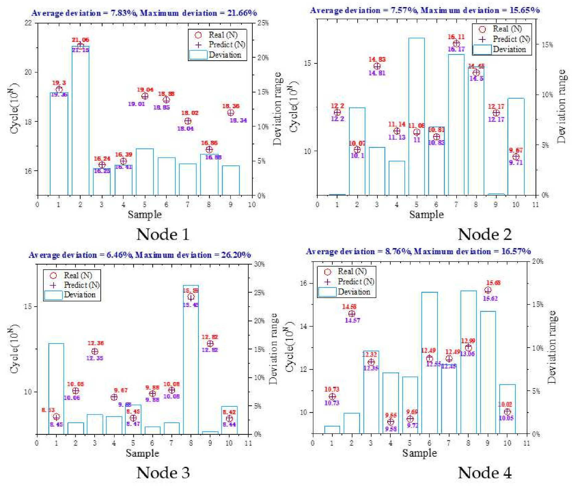
Figure 7 shows the results of the data training and test. The average deviation of the radial basis neural network is below 10%, and most of the maximum deviations are below 20%, which can be used for subsequent predictions.
3.2. Hypothesis Test for Fatigue Life Distribution
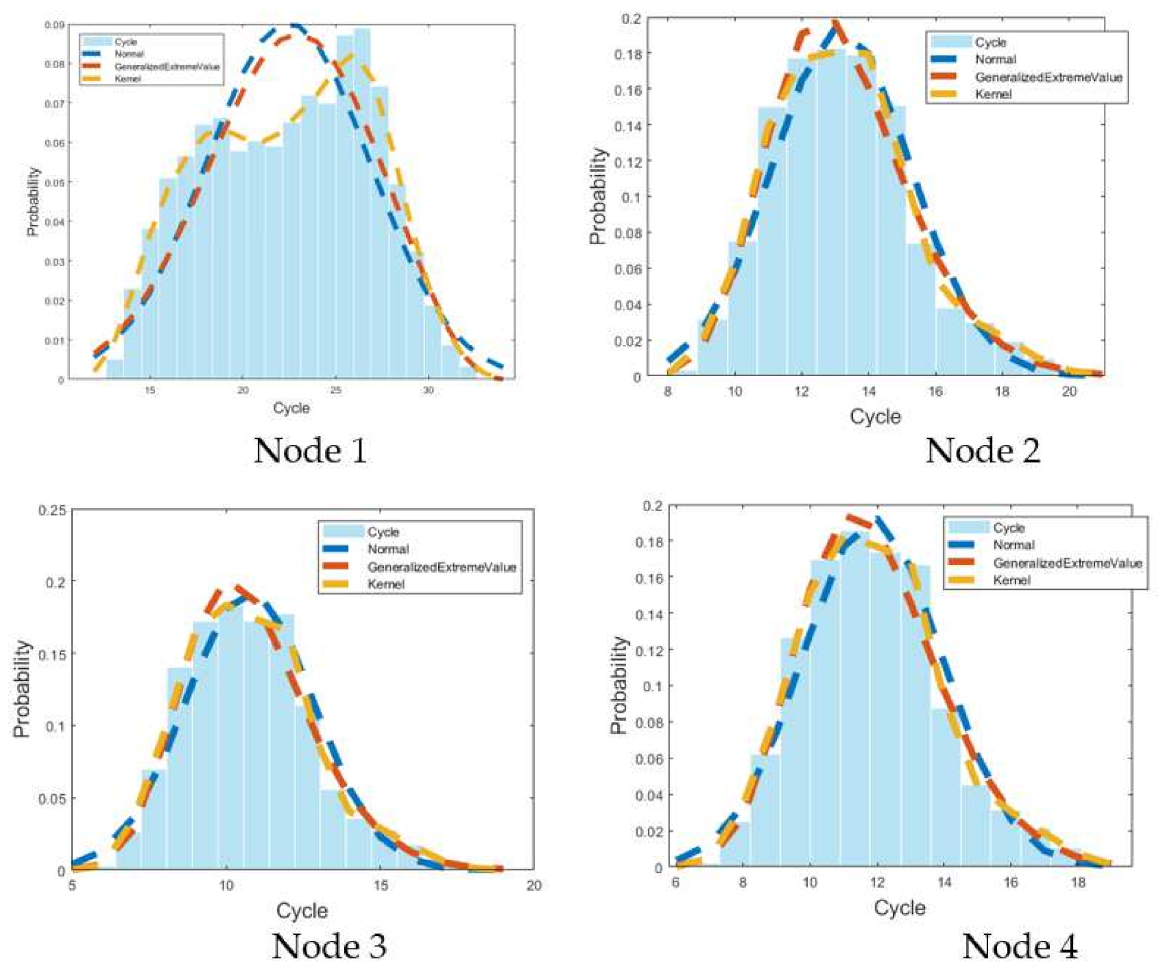
In view of the obtained RBF neural network and joint distribution model parameters of wind velocity and direction, this study predicted the life of each node of the curtain wall supporting structure, as shown in
Figure 8.
The degree of fitting is roughly judged by correlation coefficient (
R2) and mean square error (
MSE), as shown in
Table 5. It indicates the kernel distribution has the best fitting effect on nodes among all distributions, whose correlation coefficient is closer to 1 than other distributions, and the mean square error is more closer to 0. Normal distribution and GEV (generalized extreme value) distribution have a slightly poor-fitting effect on node 1, but the fitting effect on other nodes is not significantly different from the kernel distribution.
The chi-square test is an important method for goodness-of-fit and it determines whether a data sample comes from specified probability distributions and parameters are estimated from the data. In the test, data were grouped into different intervals whose actual and theoretical frequencies were calculated, and chi-square test statistic was measured [
15].
The chi-square test aims to check the difference level between actual frequency and theoretical frequency; therefore, the core content is to calculate the statistic of the overall difference between actual frequency and theoretical frequency, which is the chi-square distance. This distance is equal to cumulative sum of ratio of square of difference between actual frequency and theoretical frequency to expected frequency [
16]:
where
stands for actual frequency and
is the theoretical frequency based on a hypothesis distribution. When the frequency is large, the statistic is in an approximate chi-square distribution. The bigger chi-square value means longer distance and stronger difference. The table below explains the actual frequency and theoretical frequency calculated by each distribution. For easy comparison, the actual frequency is a positive integer, and the theoretical frequency is accurate to one decimal place.
Table 6 lists test frequencies under various hypothetical distributions, including actual and theoretical frequencies. The difference in actual and theoretical frequencies of the three distributions is far from obvious.
Provided that
unknown parameters in theoretical distribution need to be replaced by a corresponding estimator, then
, statistic
distribution is asymptotical to
distribution with
degrees of freedom, and
is the number of intervals of test data. According to the theorem, for a given significance level
, critical value
is obtained by looking up the distribution table:
If the measured value of statistic calculated according to the given sample value falls into the rejection region, the null hypothesis is rejected. Otherwise, the difference is considered insignificant and the null hypothesis is accepted.
Propose a hypothesis for statistical data of wind-induced fatigue of curtain wall: fatigue life data obeys normal distribution, generalized extreme value distribution, and kernel distribution. The default intervals are 10, 2 unknown parameters of the normal distribution, 3 unknown parameters of GEV distribution, and 1 unknown parameter of kernel distribution. According to them, the critical value
corresponding to the corresponding significance level
can be found on the quantile table on the upper side of the chi-square distribution.
Table 7 lists the chi-square test parameter calculation and search results.
It shows from the table, values of four selected nodes are all much smaller than , indicating that the null hypothesis is established, and fatigue life data obey the above three distributions. Among them, the calculated value of the chi-square distance of node 1 for three distributions is small, meaning the degree of conformity is good. On the whole, the minimum value is found in the calculation of Node 1 to the kernel distribution, which is consistent with the statistics of life probability distribution in the previous part. The maximum value appears in the calculation of Node 4 to a normal distribution, less than 1, indicating that fatigue life data are in good agreement with the three distributions.
3.3. Distribution Law of Fatigue Life
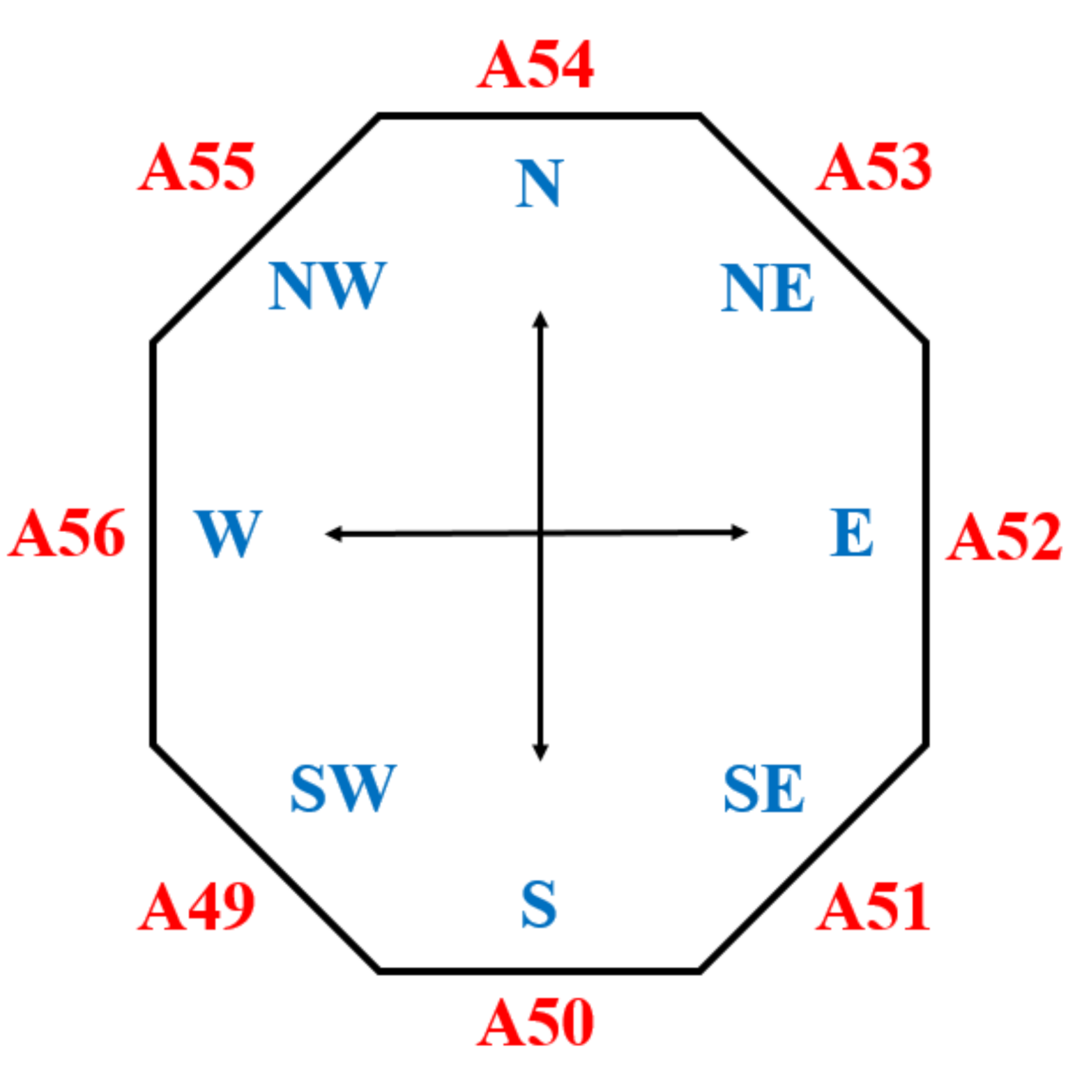
In this study, Node 4 was selected as a representative to analyze the wind-induced fatigue life distribution law of curtain wall supporting structure.
Figure 9 describes a schematic diagram of the orientation of each partition, and fatigue analysis is performed on the glass curtain wall in the northwest zone with greater stress.
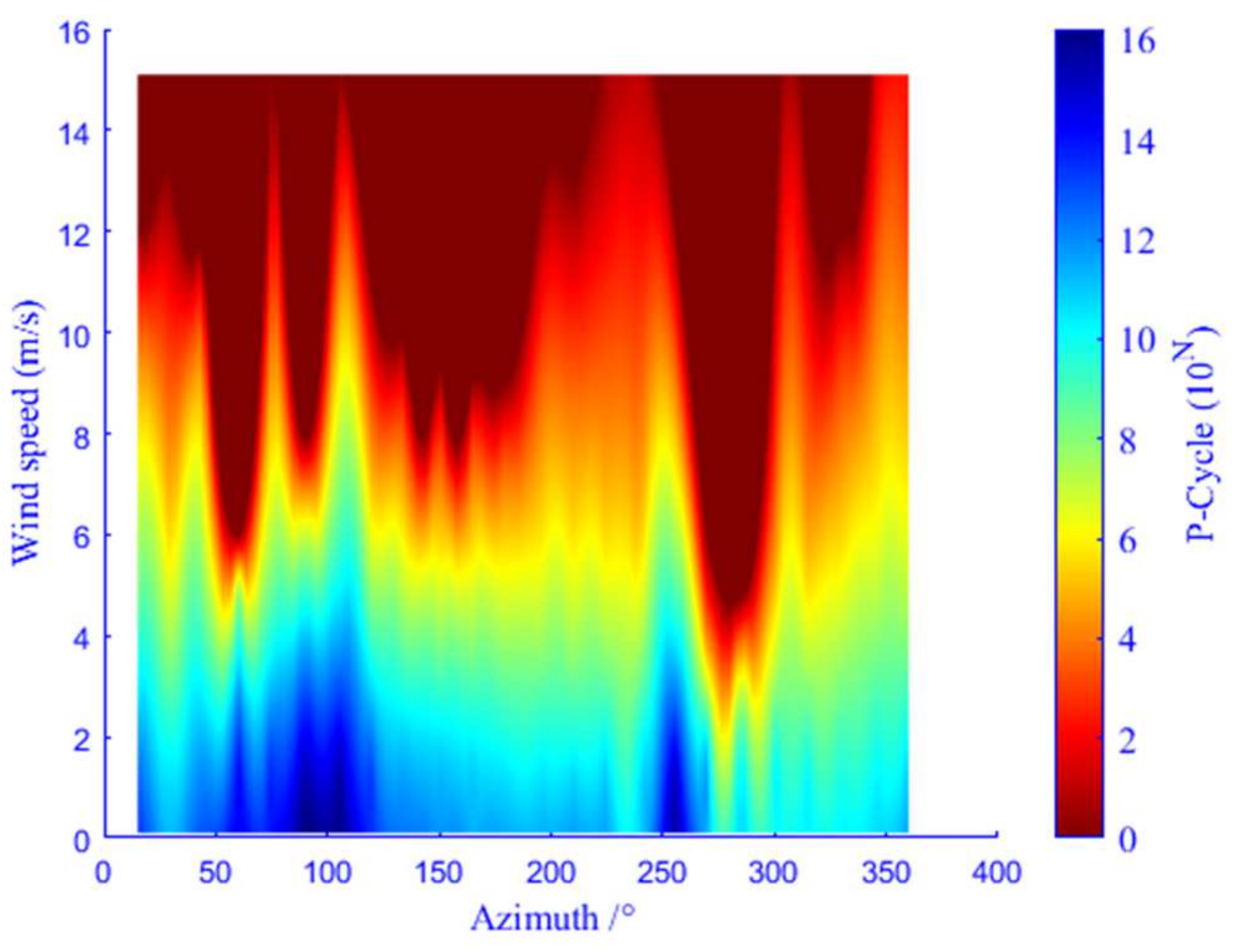
In this paper, the probability life is used to reflect the degree of fatigue damage, and the probability life (P-Cycle) is the product of the probability of the condition (Probability) and the fatigue life (Cycle). In general, the probability life of nodes in different regions is between 0~10
16 and obviously distributed in three regions. According to the probability life distribution in the northwest area (
Figure 10), working conditions with high probability life (bluish area) mainly face wind velocity 0~5 m/s and an azimuth angle between 30°~120° and 240°~260°. Working conditions with middle probability life (greenish area) mainly experience wind velocity 4~8 m/s and azimuth angle 0°~360°. Wind velocity 8~15 m/s and an azimuth angle 50°~100°, 120°~200°, and 260°~300° are found in working conditions with low probability life (reddish area), and this part accounts for the largest proportion of all probability life conditions.
Table 8 introduces 10 working conditions with shorter probability life at Node 4. On the whole, the probability life of node 4 is distributed between [10
6, 10
11]; the probability of a single working condition is generally below 0.01%, with a maximum of less than 0.02%; the azimuth is distributed between [190°, 365°], and wind velocity is between [8, 12]. According to the calculation, about 95% of fatigue damage takes place in the first 30 working conditions, and the fatigue damage value is between 3.5 × 10
−3~9.36 × 10
−2. The total damage of node 4 calculated in this paper is about 10
−3 orders of magnitude, and the fatigue damage of bolt of curtain wall aluminum calculated in the literature [
17] is between 10
−3~10
−6 orders of magnitude, which is not much different from the total fatigue damage calculated in this paper and can be used as a comparison.


