
Validating Aerosol Optical Depth Estimation Methods Using the National Institute of Environmental Research Operational Numerical Forecast Model

 , ,
, ,  ,
,
Abstract
:1. Introduction
2. Data and Methods
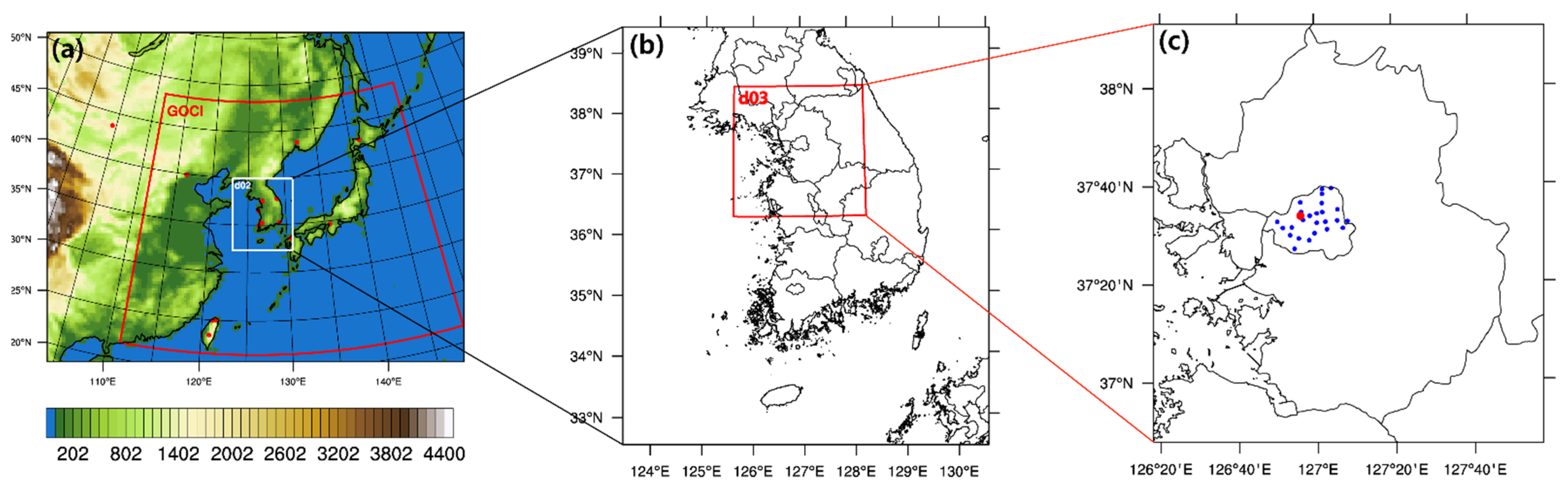
2.1. Data
2.1.1. Description of the NIER Operational Forecast Model
2.1.2. Observational Data
2.2. Estimation Methods for AOD
2.2.1. IMPROVE and Its Uncertainty
2.2.2. Other Formulations for Estimating AOD from WRF-CMAQ
3. Results
3.1. Performance of the NIER Operational Model (WRF-CMAQ)
3.2. Validation of AOD Estimation Methods
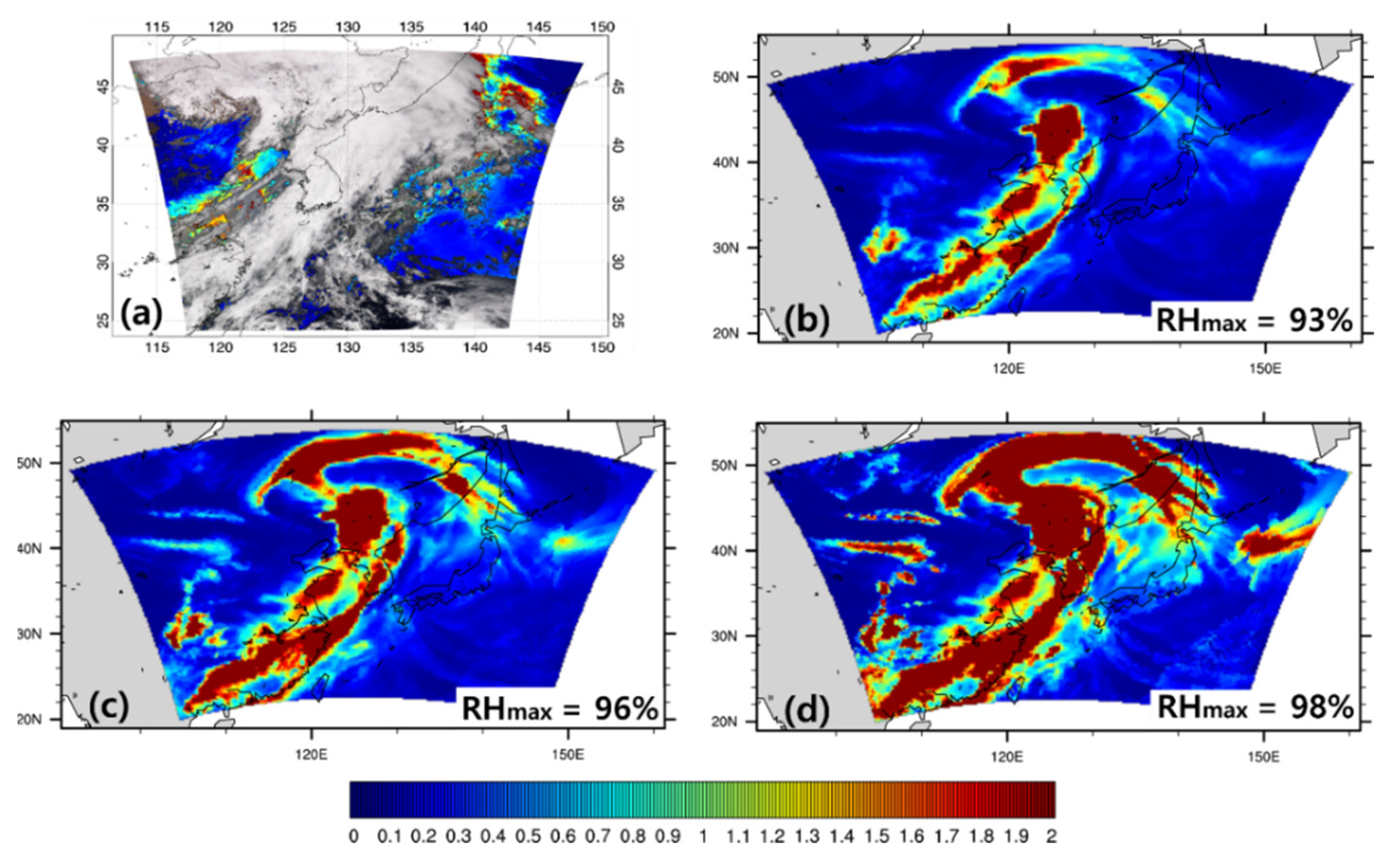
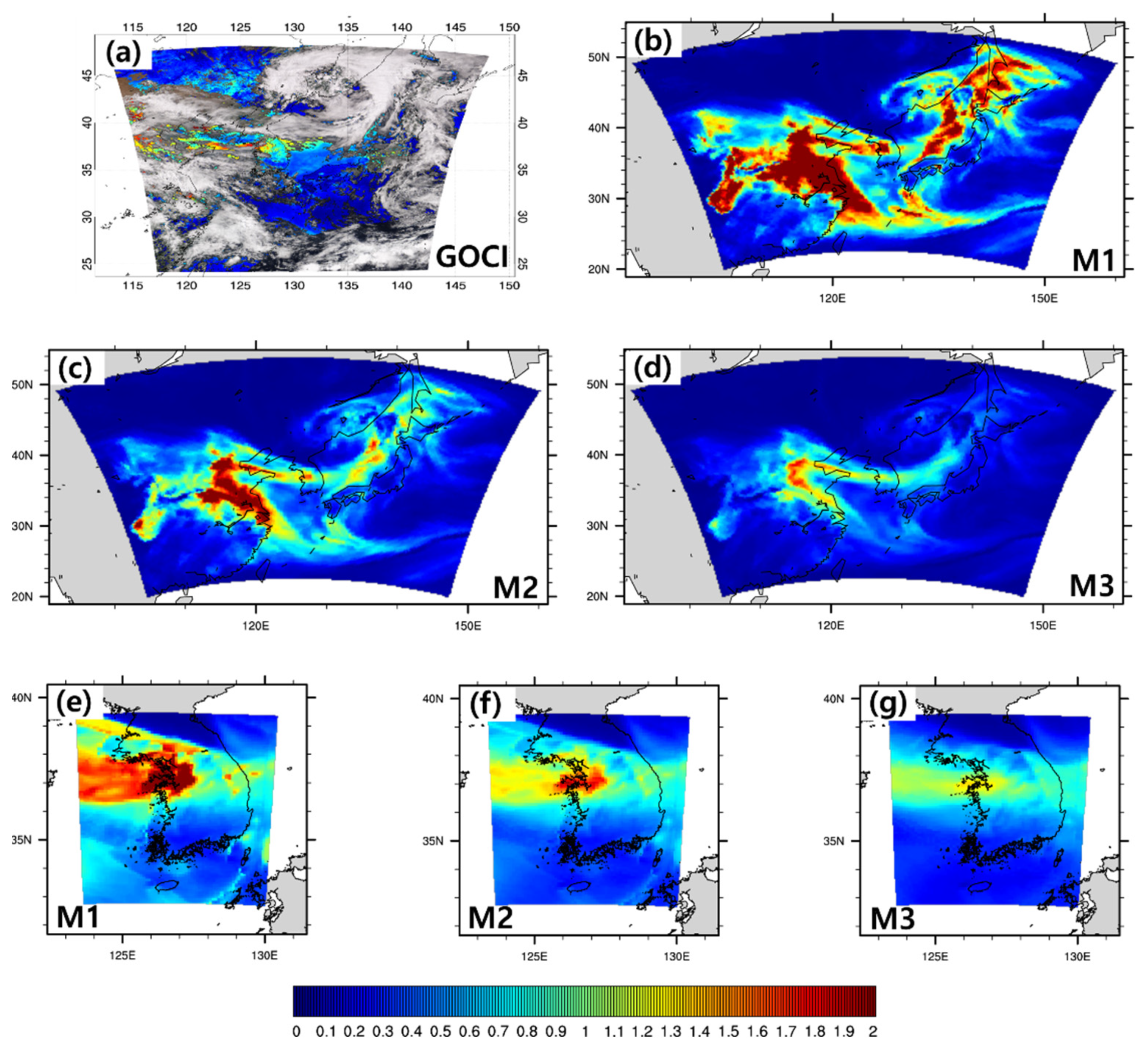
3.2.1. Springtime
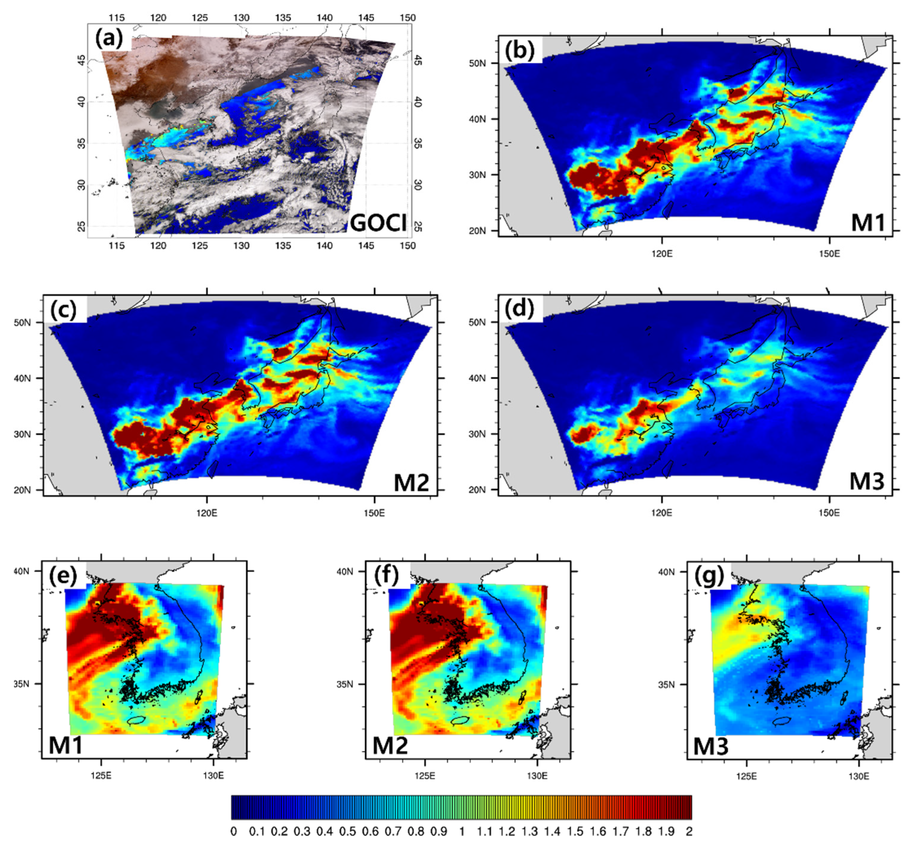
3.2.2. Wintertime
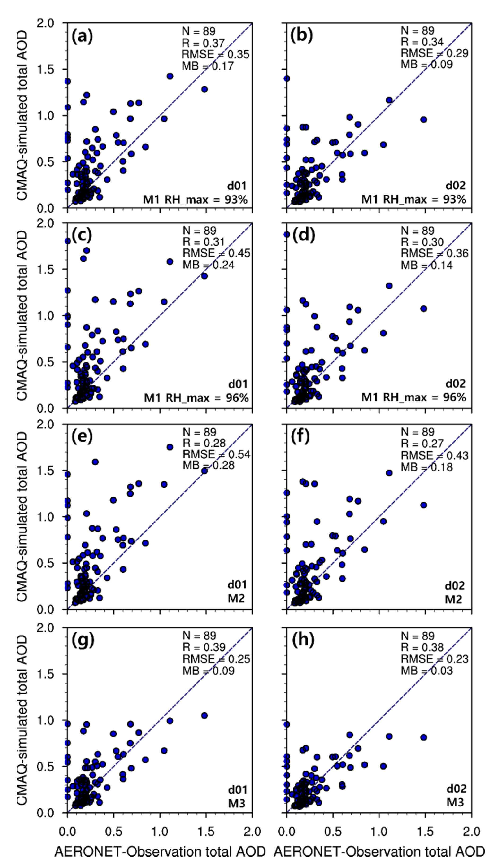
3.2.3. Statistical Analysis for the Entire Numerical Domain
4. Summary and Conclusions
Author Contributions
Funding
Institutional Review Board Statement
Informed Consent Statement
Acknowledgments
Conflicts of Interest
Appendix A

| RH(%) | RH(%) | RH(%) | ||||||
|---|---|---|---|---|---|---|---|---|
| 0~36 | 1.00 | 1.00 | 56 | 1.78 | 1.61 | 76 | 2.60 | 2.18 |
| 37 | 1.38 | 1.31 | 57 | 1.81 | 1.63 | 77 | 2.67 | 2.22 |
| 38 | 1.40 | 1.32 | 58 | 1.83 | 1.65 | 78 | 2.75 | 2.27 |
| 39 | 1.42 | 1.34 | 59 | 1.86 | 1.67 | 79 | 2.84 | 2.33 |
| 40 | 1.44 | 1.35 | 60 | 1.89 | 1.69 | 80 | 2.93 | 2.39 |
| 41 | 1.46 | 1.36 | 61 | 1.92 | 1.71 | 81 | 3.03 | 2.45 |
| 42 | 1.48 | 1.38 | 62 | 1.95 | 1.73 | 82 | 3.16 | 2.52 |
| 43 | 1.49 | 1.39 | 63 | 1.99 | 1.75 | 83 | 3.27 | 2.60 |
| 44 | 1.51 | 1.41 | 64 | 2.02 | 1.78 | 84 | 3.42 | 2.69 |
| 45 | 1.53 | 1.42 | 65 | 2.06 | 1.80 | 85 | 3.58 | 2.79 |
| 46 | 1.55 | 1.44 | 66 | 2.09 | 1.83 | 86 | 3.76 | 2.90 |
| 47 | 1.57 | 1.45 | 67 | 2.13 | 1.86 | 87 | 3.98 | 3.02 |
| 48 | 1.59 | 1.47 | 68 | 2.17 | 1.89 | 88 | 4.23 | 3.16 |
| 49 | 1.62 | 1.49 | 69 | 2.22 | 1.92 | 89 | 4.53 | 3.33 |
| 50 | 1.64 | 1.50 | 70 | 2.26 | 1.95 | 90 | 4.90 | 3.53 |
| 51 | 1.66 | 1.52 | 71 | 2.31 | 1.98 | 91 | 5.35 | 3.77 |
| 52 | 1.68 | 1.54 | 72 | 2.36 | 2.01 | 92 | 5.93 | 4.06 |
| 53 | 1.71 | 1.55 | 73 | 2.41 | 2.05 | 93 | 6.71 | 4.43 |
| 54 | 1.73 | 1.57 | 74 | 2.47 | 2.09 | 94 | 7.78 | 4.92 |
| 55 | 1.76 | 1.59 | 75 | 2.54 | 2.13 | 95 | 9.34 | 5.57 |
| RH(%) | Growth Factor | RH(%) | Growth Factor | ||
|---|---|---|---|---|---|
| 1~46 | 1.0000 | 1.0000 | 71 | 1.8434 | 3.1269 |
| 47 | 1.5922 | 2.3584 | 72 | 1.8589 | 3.1729 |
| 48 | 1.6001 | 2.3799 | 73 | 1.8751 | 3.2055 |
| 49 | 1.6081 | 2.4204 | 74 | 1.8921 | 3.2459 |
| 50 | 1.6162 | 2.4488 | 75 | 1.9100 | 3.2673 |
| 51 | 1.6245 | 2.4848 | 76 | 1.9288 | 3.3478 |
| 52 | 1.6329 | 2.5006 | 77 | 1.9488 | 3.4174 |
| 53 | 1.6415 | 2.5052 | 78 | 1.9700 | 3.5202 |
| 54 | 1.6503 | 2.5279 | 79 | 1.9925 | 3.5744 |
| 55 | 1.6593 | 2.5614 | 80 | 2.0166 | 3.6329 |
| 56 | 1.6685 | 2.5848 | 81 | 2.0423 | 3.6905 |
| 57 | 1.6779 | 2.5888 | 82 | 2.0701 | 3.8080 |
| 58 | 1.6875 | 2.6160 | 83 | 2.1001 | 3.9505 |
| 59 | 1.6974 | 2.6581 | 84 | 2.1328 | 4.0398 |
| 60 | 1.7075 | 2.6866 | 85 | 2.1684 | 4.1127 |
| 61 | 1.7179 | 2.7341 | 86 | 2.2077 | 4.2824 |
| 62 | 1.7286 | 2.7834 | 87 | 2.2512 | 4.4940 |
| 63 | 1.7397 | 2.8272 | 88 | 2.2999 | 4.6078 |
| 64 | 1.7511 | 2.8287 | 89 | 2.3548 | 4.8573 |
| 65 | 1.7629 | 2.8594 | 90 | 2.4174 | 5.1165 |
| 66 | 1.7751 | 2.8943 | 91 | 2.4898 | 5.3844 |
| 67 | 1.7877 | 2.9105 | 92 | 2.5749 | 5.7457 |
| 68 | 1.8008 | 2.9451 | 93 | 2.6769 | 6.1704 |
| 69 | 1.8145 | 3.0105 | 94 | 2.8021 | 6.7178 |
| 70 | 1.8286 | 3.0485 | 95 | 2.9610 | 7.3492 |
References
- Haywood, J.; Boucher, O. Estimates of the direct and indirect radiative forcing due to tropospheric aerosols: A review. Rev. Geophys. 2000, 38, 513–543. [Google Scholar] [CrossRef]
- Xun, L.; Lu, H.; Qian, C.; Zhang, Y.; Lyu, S.; Li, X. Analysis of aerosol optical depth from sun photometer at Shouxian, China. Atmosphere 2021, 12, 1226. [Google Scholar] [CrossRef]
- Jung, C.H.; Yoon, Y.J.; Um, J.; Lee, S.S.; Han, K.M.; Shin, H.J.; Lee, J.Y.; Kim, Y.P. Approximated expression of the hygroscopic growth factor for polydispersed aerosols. J. Aerosol. Sci. 2021, 151, 105670. [Google Scholar] [CrossRef]
- Li, J.; Han, Z.; Zhang, R. Influence of aerosol hygroscopic growth parameterization on aerosol optical depth and direct radiative forcing over East Asia. Atmos. Res. 2014, 140, 14–27. [Google Scholar] [CrossRef]
- Kim, D.-R.; Choi, W.-J.; Choi, M.; Kim, J.; Cho, A.; Kim, S.-K.; Kim, J.; Moon, K. Analysis of aerosol optical properties for high particulate matters and light Asian dust in Seoul Using GOCI. J. Korean Soc. Atmos. Environ. 2017, 33, 233–240. [Google Scholar] [CrossRef]
- Choi, M.; Kim, J.; Lee, J.; Kim, M.; Park, Y.J.; Holben, B.; Eck, T.F.; Li, Z.; Song, C.H. GOCI Yonsei aerosol retrieval version 2 products: An improved algorithm and error analysis with uncertainty estimation from 5-year validation over East Asia. Atmos. Meas. Tech. 2018, 11, 385–408. [Google Scholar] [CrossRef] [Green Version]
- Kim, J.; Kim, M.; Choi, M. Air Pollution in Eastern Asia: An Integrated Perspective. Air Pollut. East. Asia Integr. Perspect. 2017, 323–333. [Google Scholar] [CrossRef]
- Zhao, Y.; Nielsen, C.P.; Lei, Y.; McElroy, M.B.; Hao, J. Quantifying the uncertainties of a bottom-up emission inventory of anthropogenic atmospheric pollutants in China. Atmos. Chem. Phys. 2011, 11, 2295–2308. [Google Scholar] [CrossRef] [Green Version]
- Gilliam, R.C.; Hogrefe, C.; Godowitch, J.M.; Napelenok, S.; Mathur, R.; Rao, S.T. Impact of inherent meteorology uncertainty on air quality model predictions. J. Geophys. Res. Atmos. 2015, 120, 12259–12280. [Google Scholar] [CrossRef]
- Holnicki, P.; Nahorski, Z. Emission data uncertainty in urban air quality modeling—Case study. Environ. Model. Assess. 2015, 20, 583–597. [Google Scholar] [CrossRef] [Green Version]
- Huang, J.; McQueen, J.; Wilczak, J.; Djalalova, I.; Stajner, I.; Shafran, P.; Allured, D.; Lee, P.; Pan, L.; Tong, D.; et al. Improving NOAA NAQFC PM2.5 predictions with a bias correction approach. Weather Forecast. 2017, 32, 407–421. [Google Scholar] [CrossRef]
- Tang, Y.; Pagowski, M.; Chai, T.; Pan, L.; Lee, P.; Baker, B.; Kumar, R.; Delle Monache, L.; Tong, D.; Kim, H.-C. 3D-Var versus Optimal Interpolation for Aerosol Assimilation: A Case Study over the Contiguous United States. Geosci. Model Dev. Discuss. 2017, 10, 1–27. [Google Scholar] [CrossRef] [Green Version]
- Choi, Y.; Chen, S.H.; Huang, C.C.; Earl, K.; Chen, C.Y.; Schwartz, C.S.; Matsui, T. Evaluating the impact of assimilating aerosol optical depth observations on dust forecasts over North Africa and the East Atlantic using different data assimilation methods. J. Adv. Model. Earth Syst. 2020, 12, 1–30. [Google Scholar] [CrossRef] [PubMed] [Green Version]
- Cheng, F.Y.; Feng, C.Y.; Yang, Z.M.; Hsu, C.H.; Chan, K.W.; Lee, C.Y.; Chang, S.C. Evaluation of real-time PM2.5 forecasts with the WRF-CMAQ modeling system and weather-pattern-dependent bias-adjusted PM2.5 forecasts in Taiwan. Atmos. Environ. 2021, 244, 117909. [Google Scholar] [CrossRef]
- Malm, C.; Sisler, J.F.; Cahill, A. Spatial and seasonal trends in particle concetration and optical extinction in the United States. J. Geophys. Res. Atmos. 1994, 99, 1347–1370. [Google Scholar] [CrossRef]
- Pitchford, M.; Malm, W.; Schichtel, B.; Kumar, N.; Lowenthal, D.; Hand, J. Revised algorithm for estimating light extinction from IMPROVE particle speciation data. J. Air Waste Manag. Assoc. 2007, 57, 1326–1336. [Google Scholar] [CrossRef]
- Eichler, H.; Cheng, Y.F.; Birmili, W.; Nowak, A.; Wiedensohler, A.; Brüggemann, E.; Gnauk, T.; Herrmann, H.; Althausen, D.; Ansmann, A.; et al. Hygroscopic properties and extinction of aerosol particles at ambient relative humidity in South-Eastern China. Atmos. Environ. 2008, 42, 6321–6334. [Google Scholar] [CrossRef]
- Chen, J.; Zhao, C.S.; Ma, N.; Yan, P. Aerosol hygroscopicity parameter derived from the light scattering enhancement factor measurements in the North China Plain. Atmos. Chem. Phys. 2014, 14, 8105–8118. [Google Scholar] [CrossRef] [Green Version]
- Wang, X.; Shen, X.J.; Sun, J.Y.; Zhang, X.Y.; Wang, Y.Q.; Zhang, Y.M.; Wang, P.; Xia, C.; Qi, X.F.; Zhong, J.T. Size-resolved hygroscopic behavior of atmospheric aerosols during heavy aerosol pollution episodes in Beijing in December 2016. Atmos. Environ. 2018, 194, 188–197. [Google Scholar] [CrossRef]
- Zhang, Y.; Wang, Y.; Zhang, X.; Shen, X.; Sun, J.; Wu, L.; Zhang, Z.; Che, H. Chemical components, variation, and source identification of PM1 during the heavy air pollution episodes in Beijing in December 2016. J. Meteorol. Res. 2018, 32, 1–13. [Google Scholar] [CrossRef]
- Byun, D.W.; Ching, J.K.S. Science Algorithms of the EPA Models-3 Community Multiscale Air Quality (CMAQ) modeling system. United States Environ. Prot. Agency 1999, 44, 1765–1778. [Google Scholar]
- Byun, D.; Schere, K.L. Review of the governing equations, computational algorithms, and other components of the models-3 Community Multiscale Air Quality (CMAQ) modeling system. Appl. Mech. Rev. 2006, 59, 51–76. [Google Scholar] [CrossRef]
- Skamarock, W.C.; Klemp, J.B.; Dudhia, J.B.; Gill, D.O.; Barker, D.M.; Duda, M.G.; Huang, X.-Y.; Wang, W.; Powers, J.G. A Description of the Advanced Research WRF Version 3, NCAR Technical Note TN-475+STR; Technical Report; NCAR: Boulder, CO, USA, 2008; Available online: https://opensky.ucar.edu/islandora/object/technotes:500 (accessed on 18 January 2022).
- Myoung, J.; Kim, T.; Lee, Y.; Suh, I.; Jang, L. Optimization of the computing environment to improve the speed of the modeling (WRF and CMAQ) calculation of the National Air Quality Forecast System. J. Environ. Sci. Int. 2018, 27, 723–735. [Google Scholar] [CrossRef]
- Choi, K.-C.; Lim, Y.; Lee, J.-B.; Nam, K.; Lee, H.; Lee, Y.; Myoung, J.; Kim, T.; Jang, L.; Kim, J.S.; et al. Evaluation of the simulated PM2.5 concentrations using air quality forecasting system according to emission inventories—Focused on China and South Korea. J. Korean Soc. Atmos. Environ. 2018, 34, 306–320. [Google Scholar] [CrossRef]
- Carter, W.P.L. Documentation of the Saprc-99 chemical mechanism for VOC reactivity assessment- draft for review purposes only not for attribution. Contract 1999, 92, 95–308. [Google Scholar]
- Woo, J.-H. MIX: A mosaic Asian anthropogenic emission inventory for the MICS-Asia and the HTAP projects. Atmos. Chem. Phys. Discuss. 2015, 15, 34813–34869. [Google Scholar] [CrossRef] [Green Version]
- Benjey, W.; Houyoux, M.; Susick, J. Implementation of the SMOKE emission data processor and SMOKE tool input data processor in models-3. In Proceedings of the Emission Inventory Conference, Denver, CO, USA, 1–4 May 2001. [Google Scholar]
- Guenther, A.; Karl, T.; Harley, P.; Weidinmyer, C.; Palmer, P.I.; Geron, C. Edinburgh Research Explorer Estimates of global terrestrial isoprene emissions using MEGAN (Model of Emission of Gases and Aerosols from Nature). Atmos. Chem. Phys. 2006, 3181–3210. [Google Scholar] [CrossRef] [Green Version]
- Guenther, A.B.; Jiang, X.; Heald, C.L.; Sakulyanontvittaya, T.; Duhl, T.; Emmons, L.K.; Wang, X. The model of emissions of gases and aerosols from nature version 2.1 (MEGAN2.1): An extended and updated framework for modeling biogenic emissions. Geosci. Model Dev. 2012, 5, 1471–1492. [Google Scholar] [CrossRef] [Green Version]
- Chen, F.; Dudhia, J. Coupling and advanced land surface-hydrology model with the Penn State-NCAR MM5 modeling system. Part I: Model implementation and sensitivity. Mon. Weather Rev. 2001, 129, 569–585. [Google Scholar] [CrossRef] [Green Version]
- Hong, S.-Y.; Lim, J.J.-O. The WRF Single-Moment 6-Class Microphysics Scheme (WSM6). J. Korea Meteorol. Soc. 2006, 42, 129–151. [Google Scholar]
- Holben, B.N.; Eck, T.F.; Slutsker, I.; Tanré, D.; Buis, J.P.; Setzer, A.; Vermote, E.; Reagan, J.A.; Kaufman, Y.J.; Nakajima, T.; et al. AERONET—A federated instrument network and data archive for aerosol characterization. Remote Sens. Environ. 1998, 66, 1–16. [Google Scholar] [CrossRef]
- Malm, W.C.; Hand, J.L. An examination of the physical and optical properties of aerosols collected in the IMPROVE program. Atmos. Environ. 2007, 41, 3407–3427. [Google Scholar] [CrossRef]
- Malm, W.C.; Day, D.E. Estimates of aerosol species scattering characteristics as a function of relative humidity. Atmos. Environ. 2001, 35, 2845–2860. [Google Scholar] [CrossRef]
- Malm, W.C.; Pitchford, M.L.; Scruggs, M.; Sisler, J.F.; Ames, R.; Copeland, S.; Gebhart, K.A.; Day, D.E. IMPROVE III: Spatial and Seasonal Patterns and Temporal Variability of Haze and Its Constituents in the United States; Cooperative Institute for Research in the Atmosphere (CIRA), Colorado State University: Fort Coolins, CO, USA, 2000. [Google Scholar]
- Duarte, R.M.B.O.; Santos, E.B.H.; Pio, C.A.; Duarte, A.C. Comparison of structural features of water-soluble organic matter from atmospheric aerosols with those of aquatic humic substances. Atmos. Environ. 2007, 41, 8100–8113. [Google Scholar] [CrossRef]
- Lee, J.Y.; Jung, C.H.; Kim, Y.P. Estimation of optical properties for HULIS aerosols at Anmyeon Island, Korea. Atmosphere 2017, 8, 120. [Google Scholar] [CrossRef] [Green Version]
- Graber, E.R.; Rudich, Y. Atmospheric HULIS: How humic-like are they? A comprehensive and critical review. Atmos. Chem. Phys. 2006, 6, 729–753. [Google Scholar] [CrossRef] [Green Version]
- Han, K.M.; Jung, C.H.; Park, R.S.; Park, S.Y.; Lee, S.; Kulmala, M.; Petäjä, T.; Karasiński, G.; Sobolewski, P.; Yoon, Y.J.; et al. Data assimilation of AOD and estimation of surface particulate matters over the arctic. Appl. Sci. 2021, 11, 1959. [Google Scholar] [CrossRef]
- Kiehl, J.T.; Schneider, T.L.; Rasch, P.J.; Barth, M.C.; Wong, J. Radiative forcing due to sulfate aerosols from simulations with the National Center for Atmospheric Research Community Climate Model, Version 3. J. Geophys. Res. Atmos. 2000, 105, 1441–1457. [Google Scholar] [CrossRef]
- Kim, B.U.; Bae, C.; Kim, H.C.; Kim, E.; Kim, S. Spatially and chemically resolved source apportionment analysis: Case study of high particulate matter event. Atmos. Environ. 2017, 162, 55–70. [Google Scholar] [CrossRef]
- Bae, C.; Kim, B.U.; Kim, H.C.; Yoo, C.; Kim, S. Long-range transport influence on key chemical components of PM2.5 in the Seoul metropolitan area, south korea, during the years 2012–2016. Atmosphere 2020, 11, 48. [Google Scholar] [CrossRef] [Green Version]
- Yun, S.G.; Yoo, C. The effects of spring and winter blocking on PM10 concentration in Korea. Atmosphere 2019, 10, 410. [Google Scholar] [CrossRef] [Green Version]
- Song, C.H.; Park, M.E.; Lee, K.H.; Ahn, H.J.; Lee, Y.; Kim, J.Y.; Han, K.M.; Kim, J.; Ghim, Y.S.; Kim, Y.J. An investigation into seasonal and regional aerosol characteristics in East Asia using model-predicted and remotely-sensed aerosol properties. Atmos. Chem. Phys. 2008, 8, 6627–6654. [Google Scholar] [CrossRef] [Green Version]
- Park, R.S.; Song, C.H.; Han, K.M.; Park, M.E.; Lee, S.S.; Kim, S.B.; Shimizu, A. A study on the aerosol optical properties over East Asia using a combination of CMAQ-simulated aerosol optical properties and remote-sensing data via a data assimilation technique. Atmos. Chem. Phys. 2011, 11, 12275–12296. [Google Scholar] [CrossRef] [Green Version]
- Kim, S.M.; Koo, J.H.; Lee, H.; Mok, J.; Choi, M.; Go, S.; Lee, S.; Cho, Y.; Hong, J.; Seo, S.; et al. Comparison of PM2.5 in Seoul, Korea estimated from the various ground-based and satellite AOD. Appl. Sci. 2021, 11, 10755. [Google Scholar] [CrossRef]


| Configuration | Description |
|---|---|
| Model version | WRF v3.3 |
| Microphysics | WRF Single-Moment 3-class scheme |
| Cumulus convection | Kain-Fritsch |
| Longwave radiation | RRTM scheme |
| Shortwave radiation | Goddard shortwave |
| Land surface | NOAH [31] |
| PBL scheme | YSU [32] |
| Model version | CMAQ v4.7 |
| Chemical mechanism | SAPRC99 |
| Aerosol module | AERO5 |
| Chemical solver | EBI |
| Advection scheme | YAMO |
| Horizontal diffusion | Multiscale |
| Vertical diffusion | Eddy |
| Cloud scheme | ACM |
| Spring | −0.01097 | 0.78095 | 0.08015 |
| Summer | −0.18614 | 0.99211 | - |
| Fall | −0.24812 | 1.01865 | 0.01074 |
| Winter | 0.34603 | 0.81984 | - |
| Annual | 0.33713 | 0.58601 | 0.09164 |
| Resolution | Method | Season | N | R | RMSE | MB | Resolution | Method | Season | N | R | RMSE | MB |
|---|---|---|---|---|---|---|---|---|---|---|---|---|---|
| 27 km | M1 max RH = 93% | Spring | 36,696 | 0.35 | 0.34 | −0.08 | 9 km | M1 max RH = 93% | Spring | 18,036 | 0.38 | 0.29 | −0.01 |
| Summer | 44,088 | 0.66 | 0.33 | −0.10 | Summer | 22,512 | 0.37 | 0.31 | −0.08 | ||||
| Fall | 33,015 | 0.60 | 0.29 | 0.01 | Fall | 16,981 | 0.50 | 0.25 | 0.05 | ||||
| Winter | 31,425 | 0.57 | 0.24 | 0.03 | Winter | 18,013 | 0.42 | 0.23 | 0.06 | ||||
| M1 max RH = 96% | Spring | 36,696 | 0.30 | 0.41 | −0.03 | M1 max RH = 96% | Spring | 18,036 | 0.34 | 0.43 | 0.07 | ||
| Summer | 44,088 | 0.63 | 0.34 | −0.08 | Summer | 22,512 | 0.36 | 0.31 | −0.04 | ||||
| Fall | 33,015 | 0.55 | 0.32 | 0.04 | Fall | 16,981 | 0.46 | 0.31 | 0.10 | ||||
| Winter | 31,425 | 0.55 | 0.25 | 0.05 | Winter | 18,013 | 0.40 | 0.26 | 0.08 | ||||
| M2 | Spring | 36,696 | 0.33 | 0.37 | −0.04 | M2 | Spring | 18,036 | 0.37 | 0.28 | −0.01 | ||
| Summer | 44,088 | 0.60 | 0.35 | −0.01 | Summer | 22,512 | 0.32 | 0.34 | 0.02 | ||||
| Fall | 33,015 | 0.54 | 0.37 | 0.09 | Fall | 16,981 | 0.46 | 0.34 | 0.13 | ||||
| Winter | 31,425 | 0.48 | 0.37 | 0.10 | Winter | 18,013 | 0.38 | 0.35 | 0.12 | ||||
| M3 | Spring | 36,696 | 0.43 | 0.30 | −0.10 | M3 | Spring | 18,036 | 0.45 | 0.22 | −0.07 | ||
| Summer | 44,088 | 0.68 | 0.33 | −0.11 | Summer | 22,512 | 0.41 | 0.32 | −0.13 | ||||
| Fall | 33,015 | 0.68 | 0.26 | −0.01 | Fall | 16,981 | 0.56 | 0.21 | −0.01 | ||||
| Winter | 31,425 | 0.61 | 0.24 | 0.03 | Winter | 18,013 | 0.46 | 0.22 | −0.05 |
Publisher’s Note: MDPI stays neutral with regard to jurisdictional claims in published maps and institutional affiliations. |
© 2022 by the authors. Licensee MDPI, Basel, Switzerland. This article is an open access article distributed under the terms and conditions of the Creative Commons Attribution (CC BY) license (https://creativecommons.org/licenses/by/4.0/).
Share and Cite
Kim, H.-J.; Shin, U.; Choi, W.J.; Koo, J.-H.; Jung, C.H.; Nam, K.-P.; Park, S.-H. Validating Aerosol Optical Depth Estimation Methods Using the National Institute of Environmental Research Operational Numerical Forecast Model. Appl. Sci. 2022, 12, 2556. https://doi.org/10.3390/app12052556
Kim H-J, Shin U, Choi WJ, Koo J-H, Jung CH, Nam K-P, Park S-H. Validating Aerosol Optical Depth Estimation Methods Using the National Institute of Environmental Research Operational Numerical Forecast Model. Applied Sciences. 2022; 12(5):2556. https://doi.org/10.3390/app12052556
Chicago/Turabian StyleKim, Hye-Jin, Uju Shin, Won Jun Choi, Ja-Ho Koo, Chang H. Jung, Ki-Pyo Nam, and Sang-Hun Park. 2022. "Validating Aerosol Optical Depth Estimation Methods Using the National Institute of Environmental Research Operational Numerical Forecast Model" Applied Sciences 12, no. 5: 2556. https://doi.org/10.3390/app12052556